Two-dimensional spectrum estimation using the radon transform

Rochester Institute of Technology

RIT Scholar Works

Theses

Thesis/Dissertation Collections

11-3-1996

Two-dimensional spectrum estimation using the

radon transform

Jennifer Wideman

Follow this and additional works at:

http://scholarworks.rit.edu/theses

This Thesis is brought to you for free and open access by the Thesis/Dissertation Collections at RIT Scholar Works. It has been accepted for inclusion in Theses by an authorized administrator of RIT Scholar Works. For more information, please [email protected].

Recommended Citation

TWO-DIMENSIONAL SPECTRUM ESTIMATION

USING THE RADON TRANSFORM

by

Jennifer L. Wideman

B.A.

DePauw University

(1984)

A thesis submitted in partial fulfillment of the

requirements for the degree of

Master of Science in the

Chester F. Carlson Center for Imaging Science

in the College of Science

of the Rochester Institute of Technology

November 3, 1996

Signature of the Author

----,--

_

Accepted by_ _

H_ar~rY~E_._R_hO_d....!.Y

CHESTER F. CARLSON CENTER FOR IMAGING SCIENCE

COLLEGE OF SCIENCE

ROCHESTER INSTITUTE OF TECHNOLOGY

ROCHESTER, NEW YORK

CERTIFICATE OF APPROVAL

M.S. DEGREE THESIS

The M.S. Degree Thesis of Jennifer

L.

Wideman

has been examined and approved by the

thesis committee as satisfactory for the

thesis requirement for the

Master of Science degree

Dr. Roger

L.

Easton, Thesis Advisor

Dr. Zoran Ninkov

Dr. Harvey E. Rhody

THESIS RELEASE PERMISSION

ROCHESTER INSTITUTE OF TECHNOLOGY

COLLEGE OF SCIENCE

CHESTER F. CARLSON CENTER FOR IMAGING SCIENCE

Title of Thesis: Two Dimensional Spectrum Estimation Using The Radon Transform

I, Jennifer

L.

Wideman, hereby grant permission to the Wallace Memorial Library of

R.I.T. to reproduce my thesis in whole or in part. Any reproduction will not be for

commercial use or profit.

TWO-DIMENSIONAL SPECTRUM ESTIMATION

USING THE RADON TRANSFORM

by

Jennifer L. Wideman

Submittedto the

Chester F. Carlson Center for

Imaging

Science

inpartialfulfillmentoftherequirements

fortheMasterofScience Degree

attheRochester Institute of

Technology

ABSTRACT

Analternative approachto two-dimensionalpower spectrum estimation

incorporating

the

Radontransforminconjunction with each ofthe one-dimensional_periodogram,

Blackman-Tukey,

andAutoregressiveparameter estimation algorithms isexamined. The Radontransformisusedtoexpress atwo-dimensionaldatasetintermsofitsprojections

onto a set of one-dimensional radial

lines,

_{effectively reducing}the two-dimensional

estimationproblemtoaseries of one-dimensional problems. The resulting

two-dimensionalpowerspectrum estimates are comparedtotheknownpower spectrafora

varietyofdatatypes. The Radontransformapproach combined withautoregressive

parameter estimation can provide ahigh-resolutionpower spectrum_{estimate,effectively}

surpassingtheresolutionlimitationsoftheFouriermethods withoutthecumbersome implementationsofthemoredirect highresolutionestimation methodsintwo

ACKNOWLEDGEMENTS

Severalindividualsand organizationshavemadecontributions

leading

tocompletion ofthisstudy.

Firstand

foremost,

Iwishtothank_my

family

fortheircontinued

patience and _{support,particularly my husband}

Dave,

and_mychildren

Bradley

andMichael.

Withoutthecontributionsfrom my advisory_committee,Dr.

Easton,

Dr.

Ninkov,

andDr.

Rhody,

_mystudies would_undoubtedlyneverhave been

completed. I particularlythankDr. Eastonforhiscontinued support and

tremendous insightandDr.

Rhody

for

introducing

metoMATLAB. Thecontributionsfromcomputer support personnel atRITandthe

Centerfor

Imaging

Sciencewere

infinitely

valuable_{in addressing}numerous issues and obstaclesthroughoutthecourse ofthisstudy.

Inaddition, Iamindebtedto theEastman Kodak Co.fortheir tuition

reimbursement program andtheirsupport of graduate studies.

Finally,

thegenerouscontributions of child carefromnumerous

caringand competentindividualsallowed methefreedomtopursue_my

studies. I particularlythank

Elaine, Kathy,

andTerri_{for volunteering}their

DEDICATION

To

Bradley

and

Michael,

TableofContents

ListofFigures viii

ListofTables x

1.0 Introduction 1

2.0 Objectives 5

3.0 Background- Literature Review 6

3.1 NonparametricSpectrum Estimation Methods 7

3.1.1 Periodogram 7

3.1.2

Blackman-Tukey

Spectrum EstimationMethod 11

3.2 Parametric Spectrum Estimation Methods 12

3.2.1. The Autoregressive Model 14

3.2.2 AR Parameter Estimation 16

3.3 Two-dimensional Spectrum Estimation 22

3.3.1 Two-Dimensional Nonparametric Methods 23

3.3.2 Two-dimensional Parametric Methods 26

3.4 The Radon Transform Approach 30

3.4.1 DescriptionoftheRadon Transform 30

3.4.2 The Radon TransformandSpectrum Estimation 38

4.0 Approach 41

4.1 Two-dimensionaldatasets 43

4.2 Two-dimensionalspectrumestimation 53

4.3 The Radon Transform Approach 54

4.4 AssessmentofSpectrum Estimation Performance 58

4.4.1 ComparisonofSpectrum Estimation Approaches 58

4.4.2 Phase EstimationandImage Reconstruction 59

4.4.3 InvestigationofInterpolation Effects 60

5.0 Results 62

5.1

Feasibility

oftheRadon Transform Approach 65

5.2 Qualitative Performance Assessment 70

5.2.1 Data Set

#1,

"Sines"

70 5.2.2 DataSet

#2,

"Rectangle"

82

5.2.3 Data Sets

#4-#6,

"Sines+ARProcess"

88 5.2.4 Data Sets#7&

#8,

"Child1"

& "Child2"

91

5.3 Phase EstimationandImage Reconstruction ₉₃

5.4 Interpolation Effects 100

6.0 ConclusionsandRecommendations ₁₀₆

Appendix -- SoftwareListings

110

ListofFigures

3-1 Data Record Segmentation for Averaged Periodograms 10

3-2 An Autoregressive ModelofOrder 2 15

3-3 Sample Data SetfromSecond Order AR Process 15

3-4 Power Spectra ComputedfromEstimated AR Parameters 20

3-5 Integration Linesfor

Computing

aSingle Radon Transform Projection 31

3-6 Radon Transform Projections for Sinusoid 32

3-7 SinogramofRadon Transform Projections 35

3-8 SinogramandReconstructedRadon Transform for Sinusoid 35

3-9

Computing

2DFouriertransformfromtheRadon Transform 36

3-10 2D FFTandRadon/ID FFTofSinusoid 37

3-1 1 Spectrum EstimationfromRadon TransformandPeriodogram 38

3-12 Spectrum Estimation from Radon Transformand

Blackman-Tukey

Method 38 3-13 Spectrum Estimation from Radon TransformandARParameter Estimation 39

4-1 Power Spectrumof

"Sines"

Data

Set,

Computed from 2-D FFT 45

4-2 Power Spectrum Estimateof

"Rectangle",

Computedfrom2D FFT 46

4-3 Power Spectrum of"AR

Process",

Computedfrom known ARparameters 48

4-4 PowerSpectrum of"Sines+ARProcess" 48

4-5 Images: Data Set#7&

8,

"Child 1"

and"Child

2"

50

4-6 Powerspectra computedfrom 2-D FFTof"Child1" and"Child2" 50

4-7 Exampleof rho-filter usedfor oversamplingcompensation 57 5-1 Spectrum Estimatesfor"Sines"

DataSet 67

5-2 Spectrum Estimatesfor "Rectangle"

DataSet 68

5-3 Spectrum Estimates for "ARProcess" Data Set 69

5-4 Spectrum Estimatefor"Sines"

--Radon/FFT,

1&45increments 72 5-5 Spectrum Estimate for"Sines"

--Radon/FFT,

45 and135projections 72 5-6 Spectrum Estimatefor"Sines"

Radon/BTand2-D

Blackman-Tukey

75 5-7 Spectrum Estimates for "Sines"

--Radon/AR;

p=5, p=10, and p=15 76 5-8 Spectrum Estimatefor"Sines"

Radon/AR,

p=10,

45

increments 78

5-9 Spectrum Estimatefor"Sines"

-Radon/AR,

p=10, 45

and135projections 78 5-10 Spectrum Estimates for "Sines"

--Radon/AR,

128and256datapoints 80 5-11 SpectrumEstimatefor"Sines"

--Radon/AR,

p=10, 45

inc.,

128 datapoints 80 5-12 Spectrum Est. for

"Sines"; Radon/AR,

128points;

0, 45, 90,

and 135 81 5-13 Powerspectrumestimatesfor "Rectangle" fromRadon/AR 83 5-14 "Rectangle"

spectrafrom Radon/per. &

Radon/AR,

beforereconstruction 85 5-15 Normalized Radon/ARspectrum estimatefor"Rectangle" ₈₆

5-16 High-resolution Radon/ARpower spectrumestimatesfor "Rectangle" ₈₇ 5-17 "Sines+ARProcess"spectrum estimatesfrom2D FFT ₈₉

5-18 "Sines+ARProcess"

5-19 Radon/ARSpectrumEstimatesfor "Child 1"

& "Child2" 92

5-20 Estimatedphase at pixel

(33,25)

vs. ARmodel order 95

5-21 Estimatedphase at pixel

(33,25)

vs. Angular inc. betweenprojections 95

5-22 Fourier Transformestimatefor dataset#10 96

5-23 Dataset

#10,

recreatedfromestimated spectrum 98

5-24 "ARProcess" recreatedfromRadon/ARestimatedspectrum 99 5-25 Interpolationeffectsfor "Single

Sinusoid";

original&recreateddatasets 101

5-26 Fouriertransformof"SingleSinusoid" viaRadontransform 102 5-27 Fouriertransformof"SingleSinusoid" via simulatedRadontransform 104 5-28 "SingleSinusoid"

ListofTables

3-1 Levinson-Durbin Autoregressive Parameter Estimates 19 4-1 Periods& Azimuthal Angles for Twelve CosinesofDataSet #1 44 4-2 Periods & Azimuthal AnglesforThree Sinusoids ofData Sets#6-#8 49

5-1 DataSets& Spectrum Estimation Algorithms for

Feasibility

Demonstration 62 5-2 Variable Input Parameters for Spectrum Estimation Algorithms 63

1.0 Introduction

In

theory,

thepowerspectrumof a continuousfunctionisobtained

by

applicationofthe

Fouriertransformfollowed

by

a squared magnitude operation. In_practice,

however,

the

continuousfunction isrepresented

by

adiscrete dataset obtained as a single realization of

the combinationof a

(possibly)

deterministicprocess and a random process. The

continuous power spectrum mustthenbe estimatedfromthedataset

by

_{using any}of a

number of spectrum estimationtechniques.

The_{first widely}used method of spectrum estimation was_{the periodogram,} developed

by

Schusterin 1898 forthe_studyof periodicitiesintheoccurrences ofsunspots

[Schuster,

1898].

Essentially

aFouriertransformofthedataset, thismethod was _{computationally}

intensiveandthereforehadlimitedapplications priorto theadvent ofdigitalcomputers

andtheFast Fourier Transform

(FFT)

algorithmdeveloped

by Cooley

and

Tukey

[1965].

A latermethodof spectrum_estimation,developed

by

Blackmanand

Tukey

[1958],

is

basedontheWiener-Khinchintheorem

describing

the_relationshipbetweenthepower

spectrumandtheautocorrelationfunctionas aFouriertransformpair. Thismethodisan indirectapproachoffirst_estimatinga series ofautocorrelationlags fromthedatasetand

then_computingtheFouriertransformoftheautocorrelationfunction. The primary

advantage ofthismethodlies intheformoftheautocorrelationfunctionwhich_generally

peaks attheoriginand_rapidlyfallstozero.

Thus,

asmallersetof non-zerodatapoints

Boththe periodogramandthe

Blackman-Tukey

methodshave become knownas classical

spectrum estimation methodsbecause

they

arebasedontheFouriertransform. Although

eachhasproven effective and useful ina_varietyof_{applications,}

they

areboth limited in

resolution

by

the_{sampling interval}usedin obtainingthedataset.

Inthepursuit ofhigher_resolution,a number of alternative methodshave been introduced.

Theso-called parametric methods arebasedon an assumptionthat thedatasetfitsa pre

determinedmathematical modeldefined

by

a set of unknown parameters. Atheoretical

expressionforthecontinuous power spectrumintermsoftheseparameters is derived

fromthecharacteristics ofthemathematical model. The spectrum estimation problem

thenbecomes one of_estimatingthemodel parametersand_substitutingtheseestimates

intothetheoreticalequationforthepower spectrum.

Threewell-known parametricmodels aretheautoregressive

(AR),

moving-average

(MA)

and autoregressive_movingaverage

(ARMA)

models. Asindicated

by

the_{nomenclature,}

theARMAmodelismoregeneral,

incorporating

thecharacteristics ofboththeARand

MAmodels. Althougheach ofthesemethodshasbeendemonstratedtobeeffectivein

powerspectrum_estimation,theARmethodhastheadvantage of_usingaparameter

estimation algorithm

involving

alinearset of Yule-Walkerequationstoestimateboththe

magnitudeand phase spectra.

Theextension of spectrum estimationforatwo-dimensionaldatasethas been

demonstrated for boththeFourierandtheparametricmethods. _{The separability}ofthe

theperiodogram andthe

Blackman-Tukey

methods. Aone-dimensionaltransformis

simplyappliedtoeachdimensioninsuccessioninordertoobtainthetwo-dimensional Fouriertransform. Of_{course, the}resolutionlimitationsassociatedwiththe _sampling

intervalandthesize ofthedataset remain.

Althoughtheparametric methods _maypromisehigherresolution when appliedto

two-dimensional

data,

the taskof_estimatingthemodel parameters canbecumbersome. An

extension ofthelinearYule-_{Walkerequations foruse in estimatingtheARparameters} foratwo-dimensionaldatasethas beendiscussed intheliterature

[Marple, 1987], [Kay,

1988].

Analternative approachto two-dimensional spectrum estimationincorporatestheRadon

transform,a means of_expressingatwo-dimensionaldatasetintermsofitsprojections

ontoa set of one-dimensional radial

lines,

tocompresstheproblemintoa series of

one-dimensionalspectrum estimation problems. Themotivationbehindthisapproachlies in

the_{relationship between}theRadontransformandtheFouriertransform_wherebythe

two-dimensional Fouriertransformcanbecomputed

by

application oftheRadontransform to

atwo-dimensionaldatasetfollowed

by

one-dimensionalFouriertransforms_alongthe

radiallinesoftheRadontransform.

Clearly,

thismethod canbe appliedto theFourier

methods of spectrum estimation

by

_{simply replacing}the two-dimensionalFourier transformwiththeRadontransformand a sequence ofone-dimensionalFourier

transforms. Inaddition, theapplicationoftheRadontransforminconjunctionwiththe

one-dimensional parametric methods offersthe_possibilityof astraightforwardestimation

Aseriesofdata_processingalgorithmshas beenappliedtodatasets withknownpower

spectrainanefforttodemonstratethe

feasibility

oftheRadontransformapproachto two-dimensional spectrumestimation. The data processingincludedboththeFourierand

parametric spectrum estimation methods. AlthoughtheRadontransformapproach used

inconjunctionwiththeperiodogram andthe

Blackman-Tukey

methods offered no

improvementsovertheirdirecttwo-dimensionalcounterparts,theRadon/ARapproach

successfullyproducedhigher-resolutionspectrumestimatesinselected cases.

However,

thebilinear interpolation implemented intheRadontransformcomputationandthe

spectrum reconstructionintroducecomputational errors whichlimittheperformance of

theRadon/ARapproach. Inaddition,care mustbetaken_{in selecting}theangular

separationbetween Radontransformprojections astoo_manyprojections_mayobscurethe

2.0 Objectives

Theobjectivesofthisproject wereto:

demonstratethe

feasibility

oftheRadontransformapproachto two-dimensional

spectrum estimation.

qualitativelycomparetheperformance oftheRadontransformapproachto that ofthe

directtwo-dimensionalspectrum estimation approach.

Theseobjectiveswere met

by

_generatingpower spectrum estimatesfora series of

two-dimensionaldatasets withknownpower spectra

by

_{using both}theRadontransform

approach anddirecttwo-dimensionalspectrum estimationtechniques. Appropriate

comparisonsbetweenpower spectrum estimates andknownpower spectra were madefor

3.0 Background - LiteratureReview

Before consideringthe_{applicability}oftheRadontransform to thefieldof spectrum

estimation,one mustfirst

develop

aknowledgeofthevarious spectrum estimation

techniquesavailableinbothone andtwo dimensions.

Historically,

observationsofthe

periodic nature ofthelengthofthe

day,

phasesof_{the moon,} andlengthoftheyearhave

resultedinthedevelopmentofthemoderncalendar and clock. Theperiodicities

governingtheseand a_varietyof other phenomenainfieldssuch as_{sonar, geophysics,}

meteorology, climatology,oceanographyand_{astronomy may be}examinedthrough

spectrum estimates computedfroma set of observeddata. Inmost_{applications, the} data

measurements are

inherently

imbedded innoise,obscuring visibility ofthe_underlying

periodicities withinthedata. Spectrumestimation provides a means of_separatingthe

strong

frequency

components withinthedatafromthe_underlyingnoise. Thiswide

spread _{applicability}of spectrum estimationhas ledto thedevelopmentof various

methods in bothone andtwo_{(or more) dimensions.}

Theone-dimensional spectrum estimation methodshave beenseparated intotwo classes:

thenonparametric

(Fourier)

methods andtheparametricmethods, describedinsections 3.1 and3.2respectively. Theextension ofthesemethodstoatwo-dimensionaldatasetis

discussed insection3.3 alongwithabrief descriptionof other2-D spectrum estimation

methods.

Finally,

adescriptionoftheRadontransformanditsapplicationtospectrum

3.1 Nonparametric SpectrumEstimation Methods

Nonparametricspectrum estimationmethods,also referredtoasFourieror classical

methods,includetheperiodogramandthe

Blackman-Tukey

approaches. Bothofthese

methodshave been_widelyusedfor decadesina_varietyof applications.

Consequently,

the_necessaryequationsanddiscussionsof advantages anddisadvantages are availablein

numeroustextsandjournalarticles. Ofparticularinterestarethetexts

by

Steven

Kay

[1988],

andR. B. BlackmanandJ. W.

Tukey

[1958]

as well asthevideotutorial

by

S.L. Marple [1990].

3.1.1 Periodogram

Theperiodogramspectrum estimateforadiscrete datarecord_x[n] oflength

N,

developed

by

Schuster in 1898 forthe_studyof sunspot_{periodicities,}isgivenby:

2

PpER^f)

~ ~

N-\

271ifn

^x[n]e

w=0

(3-1)

For

decades,

theperiodogramwasthe_onlyavailable methodforpowerspectrum

estimation.

However,

its computational

intensity

prevented widespread use untilthe

adventofthefastFouriertransform

(FFT)

algorithmdeveloped

by

J.S.

Cooley

andJ.W.

Tukey

in 1965

[Cooley,

1965]. WhentheFFTisused,the computational_efficiencythen

The primarydisadvantagesofthismethod aretheresolutionlimitof

A/

=\/2N imposed

by

the Whittaker-Shannon_samplingtheorem

[Goodman, 1968],

thepresence of sidelobes

dueto theinherent_windowingofthe

data,

andtheunfortunatefactthattheperiodogram

isaninconsistent_estimator,

i.e.,

thevarianceoftheperiodogramdoesnotdecreaseasthe

size ofthedatasetincreases.

Theinherent_windowing ofthedata isa result oftheimplicit infiniteextension ofthedata

set_usingzero-valueddatapoints.

Essentially

theperiodogramanalysisisappliedtothe

product ofthefunctionofinterestand a unit amplitude rectanglefunction_representing

thedatawindow:

g(x)

=

f(x)

x

rect(x)

(3_2)

The resulting Fouriertransform

is,

_therefore,a convolution ofthedesiredtransformand a

sinefunction (the Fouriertransformoftherectanglefunction):

G(^)

=

F(^)*sinc(^)

(3.3)

Thisconvolution resultsinsidelobes or"leakage" of powerintoadjacent

frequency

regions.

Consequently,

thesidelobes of a_strong

frequency

component can obscure

weaker signalsat_{nearby frequencies.}

By

_selectingalternate data_windows,atrade-off

canbemadebetweenthebandwidthofthemainlobe

(resolution)

andthemagnitudeof

Onewouldexpectthatanincrease inthelengthofthedatarecord wouldimprovethe

periodogram estimate ofthepowerspectrum.

Indeed,

theperiodogramisan unbiased

estimator andthemeandoesconvergeto the truepower spectrum asthenumberofdata

pointsincreases.

However,

becausethevariance oftheestimateis a constant

[Kay,

1988],

theestimatoris inconsistent. Inordertodecreasethevarianceoftheperiodogram

estimate, thespectrum estimatesfrommultipledatasets_{may be} averaged.

Frequently,

themultipledatasets are obtained

by

_subdividingtheoriginaldataset oflengthNintoK

shorter_{non-overlapping}datasets oflength L

[Bartlett,

1948]. Theaveraged periodogram

estimate isthengivenby:

K-\

PAVPER(f)

~~/

/p^RJf)

(3-4)

m=0

where

PpEnif)

istheperiodogramoflength Lforthemthdataset

2

3S(/>4

L

L-\

(3-5)

n=0

However,

thecostofthisdecreasedvarianceisaninherent decrease inresolutiondueto

the_smoothingeffect ontheindividualperiodogramestimates.

Avariation oftheaveraged periodogramistheWelchmethod_utilizingadatawindow

and_{overlapping data}blockstoachieve additional variance reduction

[Welch,

1967]. In

this method, theoriginaldatarecord oflength N isagain segmentedintosmallerdata

records oflength

L,

_allowingthedatarecordstooverlap. Adatawindowisappliedto

estimator. Thereductionoftheestimator varianceisa result oftheincreasednumber of

datarecordsobtained

by

_allowingthesegmentstooverlap. Thesegmentationofthe

originaldatarecordforboththeBartlettaveraged periodogramandtheWelchmethodis

illustrated inFigure 3-1. Aquantitativediscussionofthereductioninvarianceforthese

averagedperiodogram methodsis containedinthetext

by

Marple,

[1987].

(a)

xx,x2,...,xL,...,xL,...x-iL; ..., x2L,

~2

T

(b)

[x\,x2,

...

,

xL\

[xL+i,xL+2,

... ,x2l]

m

'

L ' _L ' _L

+1 +2 +L

2 2 2

1

31 > N- +1

2

XIL >X3L ''X3I

+1 +2 +L

2 2 2

xN-L+\> XN

[xN-L+\

>xN-L+2' XN

]

x

3L >x

3Z. >>* L

N- +1 N- +2 N

2 2 2

Figure 3-1: An illustration ofdatarecord segmentationforaveraged

periodograms.

(a)

Schuster'speriodogram uses a singledatarecord of

lengthyV.

(b)

The Bartlettaveragedperiodogram usesthe samedata

segmentedintorecords oflength L.

(c)

The Welch averaged periodogram

3.1.2

Blackman-Tukey

SpectrumEstimation Method

Thespectrum estimation methoddeveloped

by

R. BlackmanandJ.

Tukey

in 1958 is

derived fromthewell-knownWiener-Khinchintheorem_relatingthepower spectrum and

theautocorrelationfunctionas aFouriertransformpair. The

Blackman-Tukey

power

spectrumestimateisgivenby:

M

Pbt(/)=

J^K-roe"2*'7"*

(3-6)

k=-M

where _r^

[k]

istheautocorrelationfunctionestimator givenby:

N-l-k

y\*[/i]x[

+

Jfc]

for *=0,L...,JV-1 N ___'

*=o

(3-7)

[-*]

for k=

-(N-l),-(N-2),...,-l.

and_w[k]isa real sequencetermed the

lag

window.

With_{this method,}thetaskbecomesone of_estimatingtheautocorrelationlagsand

deriving

thepower spectrum viatheFouriertransform. Therequired number of

autocorrelationlags dependsontheshape oftheautocorrelation

function,

andthusis

determined

by

thechoice ofthe

lag

window. Beforetheintroductionofthe

Cooley-Tukey

FFTalgorithmin

1965,

thecomputational_efficiency ofthe

Blackman-Tukey

estimator was a clear advantage when_onlyafewautocorrelation

lag

estimateswere

required.

However,

thedisadvantagesoftheperiodogram relatedtotheFouriertransformare still

resolutionlimitationof

A/

= 1/2 N _andthe"leakage"into _{signal sidelobes}described

by

equations

(3-2)

and(3-3). In_addition,some autocorrelation sequence estimates can result

innegative values ofthepower spectrum withthe

Blackman-Tukey

method

[Kay

and

Marple,

1981].

3.2 Parametric Spectrum Estimation Methods

Inthepursuit ofhigher_resolution, a number of parametricspectrum estimation methods

have been developed. Thepremise ofa parametric methodistheassumptionthat thedata

were generated

by

a process which canberepresented

by

a mathematical model_utilizing

a set of parameters. Atheoreticalpower spectrum canthenbe derived fromthemodel

usingthemodelparameters. Theproblem of_estimatingthepower spectrumthen

becomesone of_estimatingtheparameters oftheassumed model.

Asubsetoftheseparametric methods aretheso-called rational models:_moving average

(MA),

autoregressive

(AR),

and autoregressive_movingaverage(ARMA). Thesemodels

have beenreferredtoas rational modelsdueto thefunctionalformofthetheoretical

ARMApower spectrum:

PARMA^e

)~

b0+ble-m+---+bQe-iq(O 2

i

+ +...+

e-v

(3-8)

P

wherethecoefficients_a,and

bt

describethe_relationshipbetweensubsequentdatapoints

and_maybeestimatedfromthedata. BoththeMAandtheARmodels are special cases

oftheARMAmodel. TheMAmodel, alsoknownastheall-zero_model, assumes allthe

theAR

(all-pole)

model. Inwords, thepower spectrumPisthesquared magnitude of a

polynomial fortheMAmodel,andtheinverseof a polynomialfortheARmodel.

The ARmodelhas beenselectedforthis_{investigation primarily for its ability}todetect

narrow-bandsignals such as sinusoids.

Consequently,

theMAandARMAmodels will

notbe discussed in further detail. Additional informationonthesemodels canbe found

inthe texts

by Kay [1988]

andMarple

[1987]

or articles

by

Kay

andMarple

[1981],

3.2.1 The Autoregressive Model

As previouslystated, thepremise oftheARmethodistheassumptionthat thedatawere

generated

by

anautoregressive processdefined

by

a set of parameters. The accuracyof thisassumptiondeterminesthe_accuracyofthe_resultingpower spectrum estimate. Once

this assumptionhasbeen_{made, the}problemthenbecomesone of_estimatingthemodel

parametersforthegivendataset.

Anautoregressive processdeterminestheamplitude of each newdatapoint as a weighted

sum oftheamplitudesofthepreviousdatapoints:

x[h]=_{-__***["}

-*]+[]

(3-9)

k=\

where_x[n]istheoutput_sequence,a^isa set ofARparameters which servetoweightthe previousdata_points,and_u[n]isa white-noise

driving

sequence. Theorder ofthemodel intheautoregressive process

isp,

themaximum value oftheindex k forwhich _ak ^0.

Althoughthisequationis similarinformtoalinearprediction

filter,

its interpretation is

uniqueto theARprocess

[Marple,

1987]. Thedependenceoftheoutputsequenceon boththeinput

driving

sequence andtheprevious output valuesisdescribed_{pictorially in}

Figure 3-2. Inaddition, an exampleof adataset generated

by

anautoregressive process

of order/?=_{2 is}

shownin Figure 3-3. Theequation_governingthisprocessisobtained

by

substitutingthetwoautoregressive_{parameters, al} =0.5 and_a2 =

-0.25, intoequation

(3-9):

x[n]

= _x[n

-1]

+-x[n

[image:26.552.72.495.289.504.2]

+

u[n]-Xi

ap )"'{%.

x[n-p] AR x[n-2]

>x[n]

x[n-l]

Figure 3-2: An Autoregressive ModelofOrder p

"(l) 1.16 10 0.5x1

KIM

0 62 -2.5 -3.84 0.5x|

)&?

-.25x

M

0.96 "(3) "(4) 0.07 5.04 0.5x|

>&?

-1.26 -3.41 0.5x|

>&?

0.85 0.35

s

3.32 0.5x

?

-.25x

?

>

Figure 3-3: Sample datasetfroma second orderautoregressive

process with _ax =0.5 and _a2 =-0.25. Theprocessis initiatedatthe

leftwithx= _{10 anddriven}

Thenext_stepin

defining

theARmodelistoderivethe theoreticalpower spectrumbased

ontheARparameters. This derivation is includedina number oftextsand articles(e.g.

[Marple, 1987]

and

[Kay, 1988])

and will notberepeatedherein. The

derivation,

based

on az-transform representationofthesystemtransfer

function,

resultsintheARpower

spectrum

density

p m

PqA

P

l

+

y]ake-2nifkAt

(3-H)

k=\

where _{p^ is}thevariance oftheinput

driving

sequence []. Withthisequationin

hand,

theestimation ofthepower spectrumhas beenreducedto theestimation oftheAR

parameters andthevarianceofthewhite-noise

driving

sequence. Athoroughdescription

ofthewhite-noise

driving

sequence anditsroleintheautoregressive modelis contained

inthepaper

by

Robinson [1982].

3.2.2 AR Parameter Estimation

The literature pertainingtoautoregressivespectrum estimationincludesanumberof

methods for

determining

themodel parametersfroma set ofdata. Thepaper

by

Roman

[1981]

provides an overview of severalmethods,

including

theYule-

Walker,

maximum

entropy

(Burg),

leastsquares,parameterestimation,and maximumlikelihoodmethods.

Thechoice of method couldbe influenced

by

a number offactors

including

thedata

record

length,

the signal-to-noiseratio, andthedesiredresolution.

However,

theselection

factorforthis_studywas_{simplythe extendibility}oftheYule-_{Walkermethodto two}

Thepremise oftheYule-_{Walkermethodisthe}

following

relationship betweenthe

autocorrelationofthedataset andtheARparameters:

r^im]

- >

Qkrxx \-m~

^]

for/w > 0

k=\ p

/

<*krxx[-k] k=\

+_pa form= 0

form <0

(3-12)

r^i-m]

Selectionofthep+1 autocorrelationlagswithindices

[0,l,2,...,p]

resultsina system of

p+1 linearequations with p+1 unknowns referredto astheYule-_Walkernormal

equations,expressedhere inmatrixform:

>xJ0]

rxx[-l]

rM

^[0]

rxx\P\

^[p-l]

rxx\rP\

fxxi-p

+

l]

^[0]

"

1

"

Pco

a\

=

0

\_aP

0

(3-13)

Theominoustaskof_solvingthissystem ofequationshas beensimplified

by

taking

advantage ofthehermitian Toeplitzcharacteristics oftheautocorrelationmatrix: the

matrix complex conjugate_symmetryandtheidenticalelements_{along any}diagonal. A

matrix equation ofthis type canbe solved_{efficiently using}theLevinson-Durbin

algorithm,originally developed

by

Levinson

[1947]

forfilterdesignandpredictionunder

theauspices oftheMIT Meteorological Projectandappliedto theARmodel

by

Durbin

EachrecursionoftheLevinsion-Durbin algorithm involvescomputation ofalargerset of

autoregressive parameters and the_{corresponding} variancefortheinput

driving

sequence.

Thenotation forthecomputed autoregressive parameters_{a^ indicates} boththe recursion,

k,

andthe indexoftheARparameter,/. The Levinson-Durbinrecursive algorithmis

initialized

by

setting:

__0_

(3_14)

'-(0)

and

of=(l-krK(0)

(3-15)

with therecursionfor

k=2,3,...,p

given

by

L

k-\

rM+

^a^rJk-l)

*

(3-16)

ki =

ak-u +akk^k-u-i

for/ =_1,2,...,*- 1

(3-17)

oJ=(l-|fl_|2)oL

(3-18)

Aclear advantage ofthe Levinson-Durbinalgorithmis itsrecursioninmodel_order,

particularlywhenthe ARmodel orderisunknown; inotherwords, theprocess of

generating theparameters foranARprocessoforder_palso producestheparametersfor

allthe lower-order ARprocesses. Therecursion isrepeated until thevariance _ok is

constant

(att

=0). Asan_example,theLevinson-Durbin autoregressiveparameter

estimatescomputed forthe64-point datasetofFigure3-3 are providedinTable

3-1.

Recall fromequation

(3-10)

that themodelorder isknown

(p

=

2)

_{and the autoregressive}

parameters_governingtheprocessare_a\= _{0.5 and}

recursionisdictatedeither

by

_preselectingthemodel order(if

known)

or

by

_comparing

thedifference betweencomputedvariancesfromsuccessiveiterations oftherecursionto

an_arbitrarily smallnumber,

r,1 r,1

ck~Gk-\ < e. FortheexampleofTable

3-1,

therecursion

was allowedtocontinue untilthevariancedifferencewas smallerthans=

0.01,

although

themodel order wasknowninadvance.

akl ak2 ak3 ak4 ak5

k=\ 0.658

k=_{2 0.456}

-0.307

k=_{3 0.426}

-0.263 0.096

k=_{4 0.420}

-0.246 0.068 -0.069

=5 0.421 -0.247 0.072 -0.072 -0.015

Table 3-1: Levinson-Durbin autoregressive parameter estimatesfor datagenerated

froman order2 autoregressiveprocess with_a\ =

0.5and_aj=

-0.25. Therecursion

wasterminatedwhenthedifference invariance waslessthan0.01.

Caremustbetaken_{in selecting}themodel orderastheARspectrum estimate willexhibit

spurious peaks when alargemodel orderischosen relativetothenumber ofdatapoints

[Kay

and

Marple,

1981]. Thisisthebasisoftherecommendation

by Kay

andMarple

that themaximummodel orderbe limitedtoone-halfthedatarecordlength.

Alternatively,

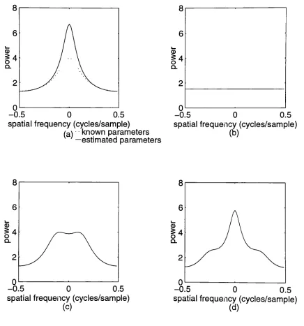
toofewautoregressive parameters_maynot yield anaccurate estimatewhen

the truepower spectrum contains _sharppeaks. Asan

illustration,

considerthepower

spatial

frequency (cycles/sample)

(a)

known parameters

-estimated parameters

-0.5 0 0.5

spatial

frequency (cycles/sample)

(b)

-0.5 0 0.5

spatial

frequency (cycles/sample)

(c)

-0.5 0 0.5

[image:31.552.60.496.97.564.2]

spatial

frequency

(cycles/sample)

(d)

Figure 3-4: Power SpectracomputedfromestimatedARparameters.

(a)

Modelorderp=2, knownparameters_aj =_{0.5 and}

a2=-0.25; estimated

parameters_ax =_{0.456 and}

a2=-0.307,

(b)

modelorderp=l,at= _0.658

(c)

model order p=3, i =

0.426,

a2=-0.263 and_a3=0.096

(d)

modelorder

Figure3-4. Boththeknownpower spectrum andthespectrum computedfromthe

estimated secondorderprocessexhibitthesame overall _shape,Figure 3-4(a).

However,

thefirstorderestimateofFigure 3_-4(b) is_constant,whilethehigherorder estimates of

Figure 3_{-4(c) and}

(d)

exhibit split peaks or sidelobes.

Anotherartifact associated withtheARspectrum estimationtechniqueistheoccurrence

ofspectralline splitting: theappearance oftwoor moredisplacedspectrallineswherea

single spectrallineshouldbeobserved. Ithas beenshown

by Kay

andMarple

[1979]

thatspectralline splittingresults fromestimation errors whentheautocorrelationis

unknown and canbe alleviatedinsome cases

by

_usingtheunbiased autocorrelation

estimatorintheYule-Walkerequations.

Asidefromtheseartifacts, theARspectrum estimation methodhasprovided an

improvementovertheFouriermethodsintermsof resolution. Marpleobservedthat the

resolution performance oftheARmodel isas much asfourtimes thatoftheFourier

methodfora20dB SNR. Theresolutiondeclined for increased_noise,

illustrating

the

sensitivityoftheARmethodto whitenoise

[Marple,

1978].

AnotherimprovementovertheFouriermethodis inthenumber ofautocorrelationlags

required. In comparingtheARmethod withthe

Blackman-Tukey,

theARmethodhas

beenshowntorequirefewer lags forthesame resolution

[Kaven,

1978]. As indicated

by

the Yule-Walkerequations,onlytheautocorrelationlags _{r_}

[m]

for

\m\

<_p arerequired

for estimatingthespectrumof an

AR(p)

process. Whenthemodel order/?is_{small, the}

3.3 Two-dimensional SpectrumEstimation

Theestimation ofspectraoftwo-dimensionalfunctions isofinterest ina_varietyof

fields,

including

sonar, radar, geophysics, andimageprocessing. The approachesto

two-dimensional spectrum estimation presented intheliteraturecanbe divided into five basic

categories:

1. directestimationusing atwo-dimensionalFouriertransform,

2. _{zero-padding followed}

by

atwo-dimensionalFourier_transform,

3. dataextrapolationbasedon a mathematical model ofthe

data,

followed

by

a

two-dimensionalFouriertransform,

4. hybridtechniqueswhich utilize aFouriertransforminonedimensionand a

one-dimensional high-resolutionspectrum estimation methodinthesecond

dimension,

and

5. non-classicaldirecttwo-dimensionalmethods.

Aswiththeone-dimensional_{methods, the two-dimensional}methods are describedina

numberof sources. Of primary interestarethetexts

by

Steven M.

Kay

[1988]

andS.L.

Marple,

Jr.

[1987]

andthearticle written

by

JamesH. McClellan [1982]. Abrief

descriptionoftheextension ofthenonparametricFouriermethodstotwo

dimensions,

including

thedataextrapolation_{technique, follows}insection3.3.1.

Theso-calledhybridor separable spectrum estimationtechniques_{usually employ}a

classicalFourierestimatorinone

dimension,

_postponingthemagnitude-squared

operation,and a modernhigh-resolutionmethodintheseconddimension

[McClellan,

methods isadequateinonedimension

(usually

temporal)

butnotintheseconddimension

(usually

spatial). Avariation onthishybridmethodincludes dataextrapolationinthe

dimensionsubjectedto theFouriermethodbefore continuingwiththehigh-resolution

methodintheseconddimension

[Joyce,

1979].

The directtwo-dimensionalmethodsincludetheparametric methods discussedearlier

(AR, MA,

ARMA)

as well asthemaximum_entropy, minimum_variance,maximum

likelihood,

PisarenkoandProny'smethods. Theextensionoftheautoregressive spectrum

estimatoris describedfurther insection3.3.2. The remainingtwo-dimensionalmethods

will notbe included inthis_studyoftheRadontransformapproach and arethereforenot

discussed further. Thereaderisreferredto the

literature,

_specifically

[Kay, 1988],

[McClellan, 1982],

[Lim and

Malik,

1981]and [Barbieriand

Barone,

1992]

foradditional

informationand resources.

3.3.1 Two-DimensionalNonparametricMethods

Thespectrum estimationtechniques_utilizingatwo-dimensional Fouriertransformare

straightforwardextensionsoftheone-dimensionalFouriertransform technique. Fora

two-dimensional dataset

f(x,y),

theFouriertransformisgiven

by

00 00

F(u,v)=

f

[f(x,y)e-2ni{xu+yv)dxdy

(3-19)

Sincethekernelofthis transformation_{is easily}separable,the two-dimensionalFourier

transformcanbeimplementedas a series of one-dimensionaltransformsas shown:

-2ni(yv) F(>v)=

l

jf(x,y)e-2ni^dx

&

(3-20)

Theperiodogramestimate thenfollows

directly

asthesquared magnitude ofthisFourier

transform.

Justas withtheone-dimensionaldiscrete_transform,theresolutionlimitsforeach ofthe

spatial

frequency

variables uand v aredetermined

by

the_samplingintervalsinthex and v

dimensions,

respectively. Zero padding (the enlargement ofthedataset with zero-valued

data points) essentiallyallowsinterpolation betweenthespectrum amplitudes obtained

fromthetransformoftheunpaddeddataset. As such, this techniquedoesnot produce

newinformation but merelypresentstheinterpolatedspectrum values atsmallerintervals.

Dataextrapolationbasedon a mathematical modelfitto thedata

does, however,

serveto

artificiallyextendthedataset. Applicationof atwo-dimensionalFouriertransform to

this larger dataset calculatesthespectrum at a smaller

frequency

interval

A/

=1/2 N ,

thus_providinghigherresolution. The accuracyofthe_resultingpowerspectrumdepends

ontheproperties ofthemathematicalmodel chosentorepresentthedata. Data

extrapolation methods include independentextrapolationforeach_{dimension [Frost}and

Sullivan

1979],

two-dimensionalextrapolationontheoriginaldataset

[Frost, 1980]

and

two-dimensionalextrapolation oftheautocorrelationfunction [Roucosand

Childers,

Extensionofthe

Blackman-Tukey

spectrum estimation methodto two dimensionsisalso

straightforward. Abiasedtwo-dimensionalautocorrelationfunction estimateisobtained

by

shiftinga_copy intwodimensionsand_summingtheproducts:

M-1-kN-l-l

}

J

x*

[m,

n]x[m+k,n +

l]

fork>0,l>0

rxx[kj]=<

MN

1

MN

m=0 n=0

M-\-kN-\

J

^

x*[m,n]x[m+

k,n

+

l]

fork>0,l<0

m=0 n=-l

(3-21)

The remainingautocorrelationfunctionestimates arebasedonthe_{hermitian symmetry}

propertyoftheautocorrelationfunction:

~*

?xx

[-k-1]

=

^xx

[k, I]

for

k

<

0,

/

>

₀

_and

k

<

0,

/

<

0

(3-22)

The

Blackman-Tukey

spectrumestimateisthengiven

by

thetwo-dimensionalFourier

transformofthewindowed autocorrelationfunctionestimate:

K L

iW(/i,/2)=

j_

Yjw[kj]Pxx[kj]e~2nKM+f2l)

k=-K 1=-L

(3-23)

Thewindowfunction _{w[k,l] is included}as ameans of_weightingtheautocorrelation

functionvalues more

heavily

forsmall

lag

values whichare computedfromthelargest

number ofdatapoints. Theautocorrelationfunctionvaluesfor higher lags arecomputed

variability. Thewindowfunctionservestoeliminatethesevaluesfromtheestimationof

the power_{spectrum, thusproviding}a spectrum estimate with alowervariance.

3.3.2 Two-dimensionalParametric Methods

Theextension oftheautoregressive spectrum estimation methodstotwodimensions

requires a parallel extension ofthemathematical model_representingthedata. Recallthat

theone-dimensional model assumesthedatawas generated

by

an autoregressive process

actingonthe_{data already}

determined,

asdefined previously inequation(3-9).

Ina single

dimension,

thedependenceof eachdatumon previousdatapointsisclear.

However,

intwoor more

dimensions,

this_relationshiptopreviousdatapointsbecomes

ambiguous.

Consequently,

parametric modelsfortwo-dimensionaldatasetshave been

developed assumingthreedifferentprediction regions: _{causal, semicausal,}and noncausal.

Eachoftheseregionsimposesa specific set of restrictions ontheindicesmand nforthe

ARparameters_amninthe_relationship

describing

theARprocess:

x[i,j] =

-____amx[i

-m,j-n] +w[i,j]

(3-24)

m n

andthe_{corresponding}power spectrumdensity:

P (f f)

AfiAfrPo

^ARUiU2)-2

l+

yya^e-2_{ni[fmAtl+f2nAt2]}

m n

where_{pffl is}the2-Dwhite noise variance.

Using

a_noncausal,orfull_plane,region of_support,theindicesmand n_maytakeon_any

integer_{value,excluding}

(m,ri)=(0,0),

_resultinginadependenceof each output_point,

x[i,j], on_potentiallyall otherdatapoints, asdetermined

by

thevalue oftheARparameter

amn. MAandARmodels_assuminga noncausal support regionhavebeen described in

theliterature

by

JainandRanganath

[1981]

andSharmaandChellapa [1986].

Boththesemicausal and causal support regions

imply

adependenceof each sample_x[i,j]

on"prior" datapoints only. Thesemicausal region assumes _{causality in only}one

dimension,

restrictingone ofthe

indices,

m or_{n, to only}non-negative values whilethe

remaining indexisunrestricted. Thisregion,thesymmetric

half-plane,

hasbeenusedin

the_study of2-D ARMA modeling

[Jain, 1981],

[Jainand

Ranganath,

1981]. The

interpretationof_{causality in}twodimensions allows either a non-symmetrichalf-planeor

a quarter-plane region of support. Themost stringentinterpretationof_causality allows

bothmand ntotakeon_onlynon-negativevalues,resulting inthefirst-quadrant

quarter-planesupport region. Similarsupport regions are alsodefined forthesecond,third, and

fourthquadrants. Itshouldbenotedthatall ofthese support regions excludetheorigin

sincetheoutput point cannot dependonitself. Thereaderisreferredto the text

by

Marple

[1987]

orthearticle

by

Jain

[1981]

formoredescriptionofthesesupport regions.

Aswiththeone-dimensionalARspectrum estimation_technique,thedefinitionof a

two-dimensional ARprocess andtheequationfor its correspondingpowerspectrum reduces

the spectrum estimationtask toone of_estimatingtheARmodel parametersfromagiven

dataset. Althoughalternative parameter estimation methodshave beenpresentedinthe

inthis _studyutilizestheYule-_{Walkernormal equations fora2-D causalARprocess:}

W

rt / i

K

for

[*.']

=

[0,0]

Z-Zr^-^-'-'-^'io

otherwise

^

i _i

wheretheindices _{/ andy}aredefined

by

_anyofthequarter-plane or non-symmetrichalf

plane support regions. Completedescriptionsofthe2-DYule-_{Walkerequationsfora}

quarter-planesupport region andtheLevinson-typerecursive algorithmfor solvingthem

are containedinthe texts

by

Marple

[1987]

and

Kay

[1988]. Itis importanttonotethat

theseequations and algorithm_closelyparallelthosedescribed forthe 1-D ARspectrum

estimation methodin Section 3.2.2. Useofthismethodthereforeprovides alogical

Itisalso importanttonotethat therestrictionof_{causality has been}shown to resultinan

ellipticallyskewed spectralresponsetoa single sinusoidinwhite noise. Acombined

quarter-planeARestimatordefinedas

1

1

+

1

'

ARCV/l'/2/ *AR1v/l'J2 /

"/U?2v/l'/2/

where

PAR

, is thefirstquadrant estimator

(3-27)

^4/?l(/l'/2)-

TJ2Pt

Pi Pi

m=0n=0

-2jii[/1mr1+/2nr2]

(3-28)

and

PAR2

isthe secondquadrantestimator

Par2

\f\^fl) ~

TJ2p

CO

0 p2

-27t/[^mr1+/2/.r2]

(3-29)

ni=ptn=0

has beenshowntoproduceacircularresponse to thesingle sinusoidinwhite noise

[Jacksonand

Chien,

1979]. JacksonandChien alsonotedtheoccurrence offewer

3.4 The Radon Transform Approach

The Radon

transform,

introducedin 1917

by

Johann

Radon,

isa meansof_expressinga

two-dimensionalfunctionintermsofitsprojectionsonto a set of one-dimensional

lines,

enablingexaminationoftheinternalstructure of an object. Sinceits

introduction,

the

Radontransformhasbeenusedina vast_arrayof_{applications,}themost_{commonly known}

being

computerized

tomography

formedical

imaging

[Kakand

Slaney,

1988]. Its

applicabilitytotheproblem of spectrum estimationisadirectresult ofthe_relationship

betweentheRadonandFouriertransformsdescribed herein. Amorethoroughdiscussion

oftheRadon_transform,itsproperties,and applicationsiscontainedinthe text

by

Deans

[1983],

which also contains a completeEnglishtranslationofRadon's 1917paper.

3.4.1 Description oftheRadon Transform

Foratwo-dimensional

function,/Tx..y)>

theRadontransformoperator is definedas a

complete set oflineintegrals_of/alongall possiblelinesL:

f{p,)

=0tf=

\f{x,y)ds

(3.30)

L

whereds isanincrementallength alongtheline L defined by:

/?=

xcos^+>-sin^

(3-31)

Thusasingle projection oftheRadontransformisobtained

by

_restricting <()to a single

value_(|>i and_{computing line integrals along}alllinesperpendicularto theradialline at

Figure 3-5: Integration lines L for computinga singleRadon transformprojectionfor(j) =_{45 degrees.}

In

theory,

theRadontransformof a continuousfunctionisalsocontinuousover all

possible values of and all linesLperpendicularto theradiallineat angle <f>. Inpractice

however,

thefunctiontobetransformedisadiscrete_matrix,or_array, of numbers. The

computedtransformwillthereforebeadiscreteapproximationto theRadontransformfor

theselected projection angles{. Asan_example,consider a sinusoidal functionwithin a

circular window as shownin Figure 3-6(a). The Radontransformprojection at =

0,

shownin Figure 3_-6(b),is computed

by

_{simply summing}overthecolumns ofthematrix.

Theperiodicnature ofthesinusoidis_clearlyvisibleinthis projection;withthedecreased

amplitudeneartheedges_resultingfromthecircular window.

Similarly

the90projection

canbecomputed either

by

_summingovertherows ofthematrix or

by

_rotatingthematrix

and_summingover_{the columns,}Figure

3-6(c)

and(d). Once again,theimpactofthe

circular windowisvisibleinthedecreasedamplitude neartheedges oftheprojection.

-1 0

100

-1 0

Figure 3-6: Radontransformprojectionsfora single sinusoid ina circular

window,

(a)

originaldata_set,

(b)

Radontransformprojectionfor =

0,

0

Q.

E CO CO

4r

2

(1

1

o

WW

-2

V

v

V

V

V

v

-4

-32 0

samples

(h)

31

Figure 3-6 (cont.):

(e)

sinusoid rotated

30,

(f)

Radon transformfor<|> =

30

constant value forthe90Radontransformprojection. Forall other projectionanglesthe

originalfunction /must berotated andfittoa set ofrectangularcoordinates before

column summations_{may be determined. Additional}rotations andRadontransform

projectionsfor

₀

= 30_{and <f>} =60_{are provided}in Figure3-6(e)-(h).

ThediscreteRadontransformismost

frequently

presentedinoneoftwoformats. The

simplestpresentationisthe sinograminwhicheachRadontransformprojectionis

represented as a singlerow ofadigitalimage. Thesinogram_containingthefour Radon

transformprojections ofFigure3-6 is the4-by-64matrixillustratedin Figure 3-7withthe

firstrow_containingthe0projection. Other Radontransformprojections_{may be}included

inthis sinogram

by inserting

(0<<}><

90)

or_{appending (<|>}>

90)

additionalrowsto the

matrix, as required. Analternative presentationis thereconstructedtwo-dimensional

Radontransforminwhicheach projectionisfilteredtocompensate_{for oversampling}near

the origin,rotated to theappropriateangle, and summedintoa single matrix. As an

illustration,

180 Radon transformprojections ((j)=

0,

1,

2,..

.,179)forthesinusoid of

Figure

3-6(a)

are presentedin both

formats,

thesinogram andthereconstructed

two-dimensional transform, in Figure 3-8.

Analternative expressionfortheRadontransform_utilizingthevectorx=

{x,y),

_the unit

vector =

(cos<{>,sin

_<))),and

employingtheDiracdelta functiontoselecttheline

/?=

c|-x,isgivenby

/(M)

=

J7W5(p-$-x)dx.

-10 0 10 20 30

samples

Figure 3-7: Sinogramwithfour Radontransformprojections forasingle

sinusoidina circular window. The fourrows representthe 64-point Radon

transform projectionsforprojectionangles =

0, 30, 60,

and90.

-50 0 50 0 200 400

Figure 3-8: Radontransformforsinglesinusoidin circular_window,

(a)

Sinogram forprojection angles<j> =

0, 1, 2,

...179.

(b)

Reconstructed

Asoutlined

by

Deans

[1983],

thisformofthe Radontransformequation canbe usedto

expressthetwo-dimensional Fouriertransformof

/(x)

intermsofthe Radontransform

and a one-dimensional Fouriertransform_alongtheradialdirection oftheRadon transform

as givenby:

F{s^)=)f{p,k)e-2^dp

(3-33)

Perhaps this_{relationship is better}understood

by

_consideringthe twopathways

leading

to

the two-dimensionalFouriertransformshown inthe

following

flow

diagram,

Figure3-9.

/(*,y)-><

Radon 1-DFourier Transform .

jF(n fc\ Transforms

OR

2-D Fourier Transform .

-*F{u,v)=

F{s

Figure3-9: Flow diagramfortwo-dimensional Fourier transform computation_usingtheRadon transform.

Thetwo-dimensionalFouriertransformsobtained_along these twopaths are

theoretically

equivalent whenthe input function

f{x,y)

iscontinuous, a sufficientthoughnot

necessarycondition.

However,

whentheinput function is adiscreterepresentation of a

continuousfunction

f{x,y),

thecomputedtransformfromeither_pathwaywillalsobea

discreteapproximationof F(u,v). The differences betweenthese two representationsare

primarily due to theinterpolationbetween datapoints _{necessary in}

fitting

thedatato a

rectangulargridforthe2-D Fouriertransformorthelines ofintegration fortheRadon

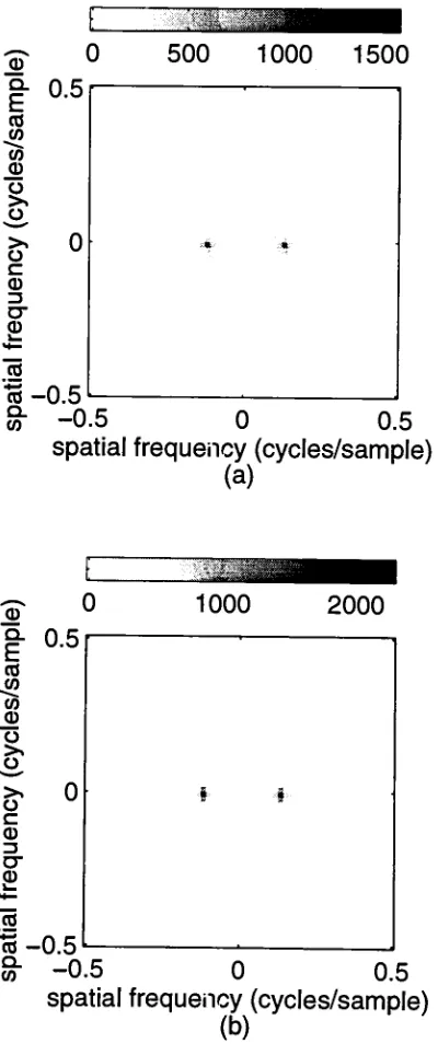
transform. The discrete Fouriertransforms forthesinusoidofFigure

3-6(a)

computed

fromthe two-dimensional FFTandfromtheRadon transformandone-dimensionalFFTs

500 1000 1500

Q.

CO -0.5 0 0.5

spatial

frequency

(cycles/sample)

(a)

co -0.5

8"

-0.5 0 0.5

spatial

frequency

(cycles/sample)

[image:48.552.175.375.75.557.2]

(b)

Figure 3-10: Fouriertransformscomputedforasingle sinusoid in acircular

3.4.2 The Radon TransformandSpectrum Estimation

Applicationofthe Radontransform tospectrum estimationinconjunction withthe

classicaltechniquesis aclear extension ofthe_{relationship between}theRadontransform

andthe two-dimensionalFouriertransform. The alternative approaches_usingtheRadon

transform inconjunctionwith theperiodogramandthe

Blackman-Tukey

methods are

illustratedinthe

following

twoflow

diagrams,

Figures 3-11 and3-12.

f(x,y)-><

Radon Transform

->/(p.O

1-DPeriodograms

)F(>5)

OR

2-DPeriodogram

F(u,v)

Squared Magnitude

,

p^fj

Figure3-11: Flow diagramforspectrum estimation

usingtheRadontransformand theperiodogram.

/U.y)--^>r_(/fc,/)->

Radon 1-DFourier Transform . /

_ _,\ Transforms

OR

2-D Fourier Transform

>->pBAfi,f2)

Figure 3-12: Flow diagramforspectrumestimation

usingtheRadontransformand the

Blackman-Tukey

method.

Theeffectiveness ofthe Radontransformapproach_clearlydependson

fitting

therotated

datato a rectangulargridbothin computingtheRadontransformprojections andin

When utilizinganon-Fourierspectrum estimation_technique,thereisnotwo-dimensional Fouriertransform to

directly

replace_usingtheRadontransformapproach.

However,

itis

areasonableexpectationthat theRadontransform_maybeusedtocompressthe

data,

or

the autocorrelation

function,

toa series of one-dimensional spectrum estimation

problems. Theflowdiagramshownin Figure 3-13 illustratestwoalternative approaches toARspectrumestimation_usingtheRadontransform.

/M

ACF

*rxx{k'l)->

Radon Transform

-\

Solve 1-D Yule-Walker

Equations

OR

Solve 2-DYule-Walker Equations

OR

Radon

Transform >/ \ 1-DACF's

>_f{P,x) *r{k)- Solve 1-D Yule-Walker

'^omn^PAR(fl,f2)

Figure 3-13: Flow diagram forspectrum estimation _usingthe

Radontransformand autoregressive parameterestimation.

Itisnotclear whetherthepremise oftheARmodel stillholdstrueforeither ofthese Radontransformapproaches. Recallthemodel assumption_{that the original}dataset was

generated

by

anARprocessdefined

by

theparameters _{amn in}equation(3-24). When

ThisinvestigationoftheRadontransformapproachto spectrumestimation addressesthe

feasibility

of_estimatingthepower spectruminconjunctionwith_{the periodogram,}the

Blackman-Tukey,

andtheARparameter estimation routines. The algorithm chosenfor

theauto-regressiveapproach isshown_alongthebottompathofFigure 3-13 flow diagram

(Radon

transform,

1-D

ACF's,

1-D Yule-_{Walkerequations). Thealternative algorithms}

4.0 Approach

Theobjective of

demonstrating

the

feasibility

oftheRadontransformapproachto

two-dimensional spectrum estimationwasaccomplished

by

_processingtwo-dimensionaldata

sets_usingdifferentspectrum estimation algorithmsand_comparingtheresultstothe

knownpowerspectrum. In_addition, aqualitative performanceassessmentincluded

comparison ofthe spectrum estimatesfromtheRadontransformapproachtoestimates

generated from directtwo-dimensionalapproaches. Theprocedure isoutlinedinthe

following

steps:

1. defineand generatetwo-dimensionalnoise-freedata

sets,

2. estimate powerspectrum_usingtwo-dimensional spectrum estimation_models,

3. estimate power spectrumusing Radontransformandone-dimensional

spectrum estimation_models, and

4. compareestimatesfromRadontransformapproachto estimatesfromdirect

two-dimensionalmethods and/orknownpower spectra.

The

feasibility

demonstration includedthreetwo-dimensionaldata sets withwell-known

power spectraas described in Section 4. 1. Inpart, thesedatasets were selectedto

examinethe_abilityoftheRadontransformapproachtoproducehigh-resolutionestimates

andto detectan_underlyingautoregressive process. Powerspectrumestimatesforthese

datasets were generatedfrom directtwo-dimensionalmethods asdescribed in Section 4.2

as well as fromtheRadontransformapproachinconjunctionwiththe_periodogram,

Blackman-Tukey,

andARparameter estimation algorithmsdescribed in Section 4.3. The

resultingpowerspectrumestimateswere examinedfortheoverallformofthe

known

Withthe

feasibility

oftheRadontransformapproach_established, a qualitative

performance assessmentincludeda comparison of spectrum estimation_approaches,an

observationof phase estimation andimagereconstruction,as well as aninvestigationof

interpolationeffects ontheestimated spectrum asdescribed in Section 4.4.

Alldata_processingwas completed_using

MATLAB,

aninteractive_programmingsystem

developed

by

The Math

Works,

Inc. SinceMATLAB_{uses matrices and vectors asbasic}

processingelements, several spectrum estimation routines were_{easily implemented}as

MATLAB_{functionscontainedin M-files. Listings ofthesesupplemental}MATLAB

4. 1

Two-dimensional

_datasets

The Radontransformapproachto two-dimensionalspectrum estimation was appliedto

sixtypes ofdatasets:

sinusoidaldata(datasets#1 & #1

1),

atwo-dimensionalrectanglefunction

(#2),

datagenerated

by

a causalautoregressiveprocess

(#3),

linearcombinationsof sinusoidal and autoregressivedata

(#4, #5, &#6),

two8-bitimages(#7 &

#8),

and

periodicfunctions

(sinusoids)

defined

by

discretedeltafunctions inthe

frequency

domain (#9 & #10).

Alldatasets were of size 64

by

64pixels.Withtheexception ofdatasets

#7-#10,

thedata

were generated_usingone(or more) oftheMATLABroutines

'planewv', 'rect2',

and

'ardata2'

aslistedinAppendix A. The'planewv'

routine generatestwo-dimensional

sinusoidaldatawith user-specified

frequency,

_{amplitude, phase, and,}azimuthal angle.

The'rect2'

functioncreates atwo-dimensionalrectanglefunctionwith auser-specified

widthin boththe

x-and y-dimensions.

Alternatively,

adatasetgenerated

by

a

first-quadrant,causalautoregressive process canbe obtainedfromthe'ardata2'

routine_using

theuser specified autoregressive parameters and aninputmatrix of randomnumbers.

The processingwas completed_{using data}sets with no additive noise inordertomeetthe

Data Set #1: "Sines"

This datasetconsistsof alinearcombination oftwo-dimensional bipolarcosines chosen

toillustratetheresolution performance of each spectrum estimation algorithm. Atotalof

twelvecosines of equal amplitudeand zero phase areincludedinthedataset. Theperiod

andazimuthal angleforeach cosine wave are listedin Table 4-1.

Period Azimuth Period Azimuth

(samples)

(degrees)

(samples)

(degrees)

la. 8 0 4a. 64/20 0

lb. 64/6 0 4b. 64/21 0

2a. 64/20 90 5a. 8 90

2b. 64/22 90 5b. 64/7 90

3a.

64/sqrt(72)

135 6a.

64/sqrt(72)

45

3b.

64/sqrt(128)

135 6b.

64/sqrt(98)

45

Table 4-1: Period andAzimuthal Anglefor Cosines ofData Set #1

("Sines")

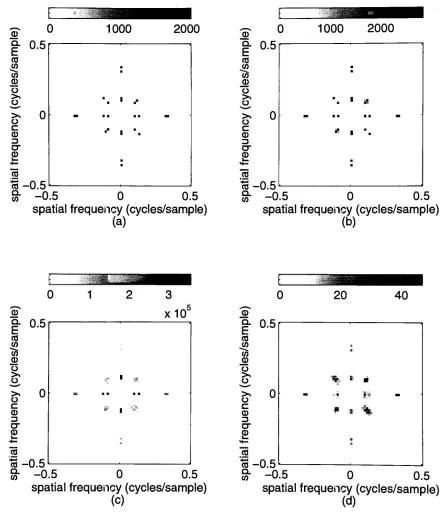
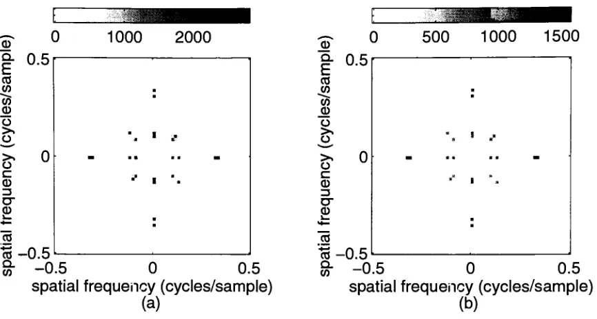
Thepower spectrum associated withthisdataset consists ofthe twelvepairsofdelta

functionsshowninthe

discrete,

gray-scale representation ofFigure 4-1. The delta

functionpairs _{corresponding}tosix ofthecosines are separatedfromanotherpairinthe

sampled

frequency

domain

by

twosamples. The delta functionpairsforthe_remaining

cosineshavea

frequency

separationof_only onesample,beyondtheresolutionlimitof

0 500 1000 1500 2000

-0.5 0 0.5

spatial

frequency (cycles/sample)

Figure 4-1: Powerspectrumfor

"Sines"

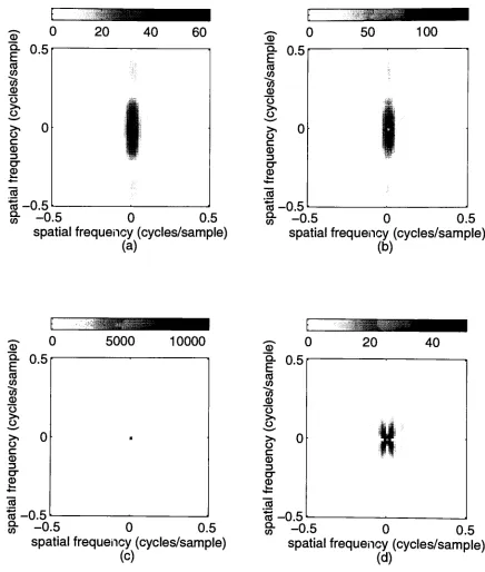
Data Set #2: Two-dimensionalRectangle Function

The seconddataset consistsof a unit-amplitude rectanglefunctionchosenforits

well-knownandrecognizableFourier_transform,thesinefunction. Thenon-zero portion of

therectanglefunction iscenteredinthematrix at pixel

(33,33)

andhaswidths of16

samples_alongthex-axis and4samples _alongthey-axis. Thepower spectrum estimate

forthisrectanglefunctioncomputed_usingthe2-D FFTisshownin Figure 4-2. As

expected, thecharacteristic shape ofthesinefunctionis _easilyobservedinthis spectrum

estimate.

0 20 40 60

-0.5 0 0.5

spatial

frequency (cycles/sample)

Figure 4-2: Power Spectrum estimatefor"Rectangle"

function,

computedfrom

Data Set #3: "ARProcess"

Thisdatasetcontainsdataobtained

by

applicationofa causal autoregressive processin

thespatialdomaintoa64-by-64matrixof normally-distributed random numbers obtained

fromtheMATLABroutine'randn'. The ARprocessis defined

by

theparameters

1 -0.5

p= -0.5 025 0

0.25 0 0

(4-1)

Sincethe autoregressive parameters are

known,

thepowerspectrum canbe_easily

computedfromequation(3-25). The author-generatedMATLABroutine'arspec2'

providedinAppendix Acomputesthispower spectrum attheuser-specified number of

frequency

points. A64-by-64

discrete,

gray-scale representation ofthepower spectrum

computedfromthear parameters isshowninFigure 4-3.

Data Set #4- #6: "Sines+AR

Process"

Thenextthreedatasets arelinearcombinationsofthe"ARProcess" dataset_previously

describedandthree sinusoids withfrequenciesand azimuthal angles chosenforthe

locationoftheirspectral peaks. Thefirsttwosinusoidshave spectralpeaks_alongthe

verticalandhorizontalaxes. The spectralpeaks associated withthethirdsinusoidare

located alongthe 45

radial lineinordertocoincidewiththepeaknon-zero regionsofthe

ARprocess spectrum shown_previouslyinFigure4-3. Theperiods andazimuthal angles

Q.

CO -0.5 0 0.5

spatial

frequency (cycles/sample)

Figure 4-3: PowerspectrumofAR_process,computedfrom known

autoregressive parameters.

CO -0.5 0 0.5

[image:59.552.198.393.75.287.2]

spatial

frequency

(cycles/sample)

Period

(samples)

Azimuthal

Angle(Degrees)

6.4

3.2

64/sqrt(200)

0

90

45

Table 4-2: PeriodsandAzimuthal Angles for Three Sinusoids ofData

Sets #4- #6

A

discrete,

gray-scale representation ofthepower spectrumisshownin Figure 4-4. It

shouldbenotedthat thenon-zerodatapoints ofthe truepower spectrum ofthe

continuoussinusoids are infinitely-valued. Thefinitevalue assignedtothesepointsin

estimatingthepower spectrumisafunctionoftheamplitude oftheinputsinusoids. The

sinusoidsin datasets

4, 5,

and6 haveequal amplitudes of

1.0, 0.5,

and

0.25,

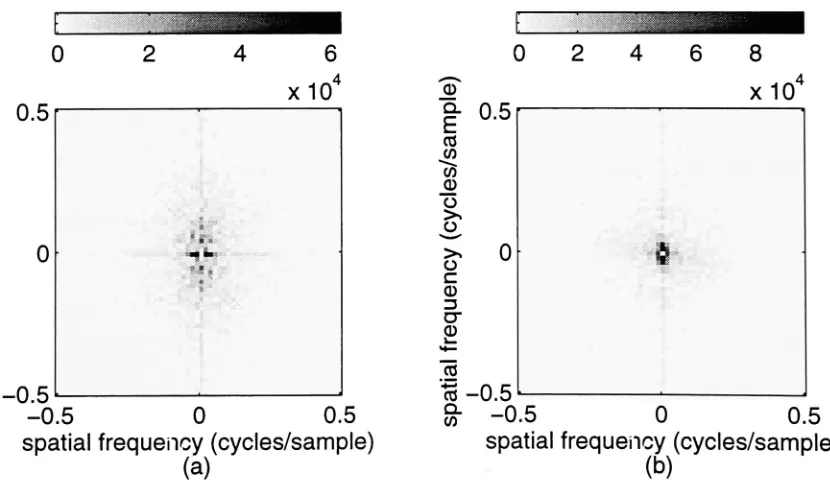
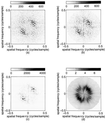
respectively.

DataSet #7and#8: Images

Thetwo_{remaining data}setsaredigitizedversionsoftwophotographs. The 8-bit images

"child 1" and"child2" showninFigure 4-5 were chosen as afirstattempt at

demonstrating

the

feasibility

of_utilizingtheRadontransformapproach with actualimage

data. Resultsobtainedfrom_{processing these two}imagesare notconsideredtobe

representativeoftheresults obtainablefrom processingallimages. Sincethe truepower

spectrumofthecontinuous signal_producingeachoftheseimages isnotknownin

advance, thespectrum estimates obtainedfromthe2-D Fouriertransformsof eachimage

are providedinFigure4-6. Itshouldbenotedthatthelinesvisible_alongthehorizontal

and vertical axes ofthesespectrum estimates are a result oftheassumedperiodic nature

-100 0 100 -100 0 100

Figure4-5:

(a)

Dataset

#7,

"Child1"

(b)

Dataset

#8,

"Child2"

Q.

CO -0.5 0 0.5

spatial

frequency

(cycles/sample)

(a)

Q.

CO -0.5 0 0.5

spatial

frequency (cycles/sample)

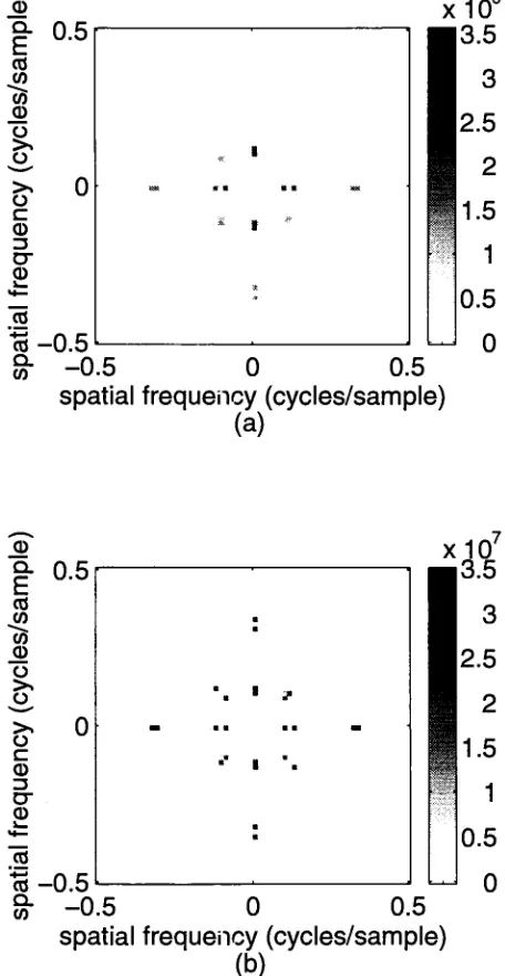
(b)

Figure4-6: Powerspectracomputedfrom 2D FFT f