Quantifying unrecognised replication present in reports of HIV diagnoses

QUANTIFYING UNRECOGNISED REPLICATION PRESENT IN

REPORTS OF HIV DIAGNOSES

Nikolaos Sfikas1, David Greenhalgh2, Wenwen Huo2, Janet Mortimer3 and Chris. Robertson2,4

(1)Novartis Pharma AG, Basel, Switzerland.

(2) Department of Mathematics and Statistics, University of Strathclyde, Livingstone Tower, 26 Richmond Street, Glasgow G1 1XH, UK.

(3) Health Protection Agency – Communicable Disease Surveillance Centre (HPA – CDSC), Colindale, London, U.K, retired.

(4) Health Protection Scotland, 5 Cadogan Street, Glasgow G2 6QE, UK.

New diagnoses of HIV infection were reported confidentially to the Public Health Laboratory Service (PHLS) AIDS Centre under a national voluntary surveillance scheme. Two sets of data drawn from the national datasets were made available to us for analysis, the first in 1991, the second in 1994, by which time the replication of reports had been reduced. The data used in the analyses consisted of the numbers of replications of the reported full date of birth in the individual records (one, two, three and so on), for each year of birth. This paper uses a non-parametric maximum likelihood estimation method for quantifying the amount of replication in the data. The estimated amount of replication was 3.37% (95% confidence interval (0.98%,11.83%)) in the 1991 and 0.58% (95% confidence interval (0%,2.64%)) in the 1994 dataset.

Keywords: HIV; AIDS; replication; maximum likelihood estimation; database

1. BACKGROUND

Acquired Immune Deficiency Syndrome (AIDS) is a severe, life-threatening

clinical condition. It was first recognised in 1981 and the virus which causes the

disease, the Human Immunodeficiency Virus (HIV) was discovered in 1983 [1, 2].

HIV is commonly spread by sexual contact, by injecting drug use, from mother to

child and by blood transfusion. Because the largest proportion (about three quarters)

of all HIV infections happen through sexual contact, HIV is considered a sexually

transmitted infection (STI) [3]. It is estimated that a total of 2.7 million people

globally acquired HIV in 2010, down from 3.1 million in 2001 and that by the end of

2010 an estimated 34 million people in the world were living with HIV [4].

The incubation period from HIV infection to AIDS is usually long and

variable with a mean of around ten years [1] and with a 95% confidence interval for

this mean being [8.4,11.2] years [5]. This means that HIV infected individuals may

remain ignorant of their infection for long periods of time, during which they may

unknowingly transmit the virus. As HIV is an STI, there is a social stigma attached to

a diagnosis of HIV or AIDS. These factors make it difficult to obtain both reliable

Since the mid 1990s there have been combinations of antiretroviral drugs

available which delay the onset of AIDS and increase the lifespan of HIV infected

individuals, but a cure for the disease is yet to be found. Data on HIV and AIDS cases

in England, Wales and Northern Ireland used to be collected by the Public Health

Laboratory Service (PHLS), Colindale, London and for Scotland by the Scottish

Centre for Infection and Environmental Health (SCIEH), Glasgow. Because of the

sensitivity concerning knowledge of an individual’s HIV status, the name of the

patient was not held in the databases. On the other hand, because of the serious social

and economic cost to both the individual and the nation, it is important that the

information available on the number of diagnosed HIV infections is as accurate as

possible [6]. In Section 2 we shall discuss the problem of recognising the extent of

undetected repeated reporting of the same individual and the previous work of

Greenhalgh, Doyle and Mortimer which is very relevant to the work presented here.

2. THE REPLICATION PROBLEM AND PREVIOUS WORK

2.1 The replication problem

A report of all individuals diagnosed as HIV positive was requested by the

PHLS, usually through the completion of a short form. The name of the individual

was not recorded on this report but the inclusion of both the date of birth and the

“Soundex” code (a four character alphanumeric code of the surname) was requested

[7]. In 1990 only a third of the records on the database held both Soundex code and

full date of birth and at that time the Soundex code was available for only about half

the database (Mortimer, 1996, personal communication). Often a local identifier, such

as a clinic number, which allowed follow up for the missing information, had been

given instead. Even when one or both of the Soundex code or date of birth were

available there is still the possibility of mis-recording or transcription errors. It was

also likely that some individuals were being repeatedly counted in the database due to

having two or more HIV positive tests reported.

There are at least two reasons why an individual already diagnosed as HIV

positive may be tested again. Firstly an individual may be unwilling to believe the

result and may seek independent confirmation of it by being tested again elsewhere.

Secondly, an individual who reports to a new GP or a new clinic as HIV positive is

could to eliminate multiple counting of such individuals in the database but it wished

to be aware of evidence of any multiple counting that still existed. This is not just a

hypothetical problem; there is at least one example of an individual having five

independent positive HIV tests reported, and it is known that mistakes in Soundex

coding and name changes result in records of the same individual remaining

unmatched despite the presence of a Soundex code on both records.

The PHLS was interested in a statistical method to test whether individuals

were being repeatedly counted in the database from the date of birth data available

and in 1991 sent us relevant information from the database as it stood then. This

consisted, for each birth year, of the number of birth dates in that year for which there

was at least one record in the database and the number of records corresponding to

that birth date in the database. No information on Soundex codes or the lack of them

for these records was sent to us at that time. The information sent to us in 1991 is

displayed in Table 1 in Appendix A. If a given birth date occurs twice in the database

it is not possible to tell from this information whether this multiple recording

corresponds to one individual recorded twice, or two distinct individuals with the

same birth date, and birth dates that occur three times or more in the database have a

greater number of possible similar ambiguities. However from the observed statistical

distribution of recorded birth dates it is possible to make inferences on whether

statistically significant replication of individuals is present and to attempt to estimate

the amount of such replication. Between 1991 and 1994, the PHLS was able to

improve the quality of their database, both prospectively by ensuring that both date of

birth and Soundex code were available for as many new cases as possible, and

retrospectively by obtaining Soundex code or date of birth or both to complete reports

received previously. This has allowed the elimination from the data of further

multiple recording of individuals. In 1994 information from the entire database as it

stood then was sent to us for further statistical analysis. This data is displayed in Table

2 in Appendix A.

HIV surveillance systems have of course advanced since 1994. As well as the

New Diagnoses reporting system described above the Health Protection Agency

(HPA) and Public Health England (PHE), the successors to the PHLS, have

cross-sectional annual surveys of prevalent diagnosed HIV infections (SOPHID). These

collect reports of all individuals in a calendar year, including those who move area,

Wales and Northern Ireland. Neither surveillance system collects names but a

Soundex code of the surname, sex and date of birth are held as identifiers [8,9].

2.2 Literature Review

We now give a brief review of work by other authors in the general area of

this problem. Larsen [10] discusses estimation of the number of people in a register

from the number of birth dates when unique identifiers are not available and when

multiple entries can occur. A method for estimating the number of registered people

is presented when dates of birth (day, month and year) are available. Registration of

people who are HIV positive is cited as an appropriate example.

The problem is clearly related to classical occupancy theory, where r balls are

placed at random in n boxes and the probability of m empty boxes is studied. Here r

has a fixed value whereas Larsen is interested in estimating r. Larsen defines n to be

the number of consecutive days in a sequence of possible birth dates; r is the number

of registered people born in the sequence; b is the number of occupied birth dates in

this sequence; and m=n-b is the number of empty birth dates in this sequence. Larsen

chooses the approximate maximum likelihood estimate,

rˆ₀(m,n)=nloge(n/m)

with approximate variance

V(r₀)~ne−r/n.

An alternative approach is discussed in which r is taken to be a random variable

reflecting the stochastic nature of registration.

Numerical calculation showed a negative bias for the true maximum

likelihood estimator rˆ and a small positive bias for the approximate maximum

likelihood estimator rˆ0. For fixed r the exact maximum likelihood was seen to be

very near the approximate maximum likelihood estimate, at least for values of n near

100. As an example registrations of Chlamydia infections were considered.

The problem which we are studying can be thought of as related to a record

linkage problem [11,12]. This addresses the problem of matching two files of

individual data under conditions of uncertainty. Individual record linkage involves

two files: file A and file B with records pertaining to individual cases [13]. Each

individual file is assumed to contain no duplicate records. Obviously, one or more

on surname and age, both files must contain fields with this information. The

objective of the record linkage process is to decide for each pair of records whether it

is a matched or unmatched pair.

A linking variable is a single criterion (such as birth date) utilized to establish

or partially establish record linkage [14]. There are two basic methods for record

linkage: deterministic linkage, which is effected only when there is an exact match on

all linking variables, and the more complex probabilistic linkage, which affects

linkage through evaluation of frequencies for linking variable values. Each time that a

new set of records is added to the database we are in effect linking two datafiles, the

old database and the new records [15]. In general probabilistic data linkage methods

are useful in that they can help us rank agreement between different matching

variables and they can also be used to incorporate effects such as data transcription

errors [13]. However they are not very relevant to the problem of assessing residual

duplication in the dataset supplied to us which had just one linking variable (the date

of birth), particularly when each value of that linking variable is equally likely.

The efficiency of probabilistic data linkage can be measured by the positive

predictive value which is the fraction of linked records which are actually true

positives. Blakely and Salmond [16] describe a “duplicate method” to calculate this

statistic when each record can be involved in only one match (for example linking

population files to death files). Elmagarid, Ipeiritos and Verykios [17] survey methods

for deterministic and probabilistic record linkage. They describe algorithms for field

matching. They point out that probabilistic data linkage can be regarded as a Bayesian

inference problem and describe a likelihood ratio based Bayes decision rule that gives

minimum error. They also discuss supervised and unsupervised learning to classify

data linkage and other methods.

Ades et al. [18] describe how an unlinked anonymous neonatal seroprevalence

survey was used with electronic record linkage to assess HIV prevalence in the UK.

In more recent work Rice et al. [9] created a cohort of HIV-diagnosed adults by

deterministically linking records across the 1998 to 2007 SOPHID database. The

records were also linked to the New Diagnoses database and to Office for National

Statistics death records. This was done to examine HIV-service attendance. This is

related to the problem studied in this paper as the problem of residual duplication may

Methods to estimate the extent of duplication would therefore be of huge help in

providing information on potential bias corrections.

Sometimes it is accepted that the data are imperfect and alternative statistical

approaches are used to compensate. For example Goubar et al. [19] estimate HIV

prevalence and proportion diagnosed in England and Wales. They take a Bayesian

approach with informative priors to synthesise different sources of surveillance

information, including the SOPHID database, using Markov Chain Monte Carlo

methods. They find that there are inconsistencies in the data but these can be resolved

by bias correction. Presanis et al. [20] use this approach to estimate prevalence and

incidence of HIV amongst men who have sex with men in England and Wales. This is

also related to the problem discussed here for similar reasons as discussed above in

relation to the HIV databases of Rice et al.

The problem considered here is not the design of a data linkage mechanism,

but rather to assess the efficiency of the data linkage already done in eliminating

duplicate reports. Technically our problem is a data linkage one, but there is only one

linking variable, date of birth, whereas normally there are several. Deterministic

linkage would simply match all records with the same birth date, which would

overlink. On the other hand there is not enough information contained in the linking

variable for probabilistic linking to be useful. Thus classical data linkage techniques

are not appropriate. We shall use maximum likelihood methods to estimate the

percentage overcounting present.

2.3 Previous work

We briefly summarise the work of Greenhalgh, Doyle and Mortimer which

shows that replication is present in the datasets. The first of these papers [21]

examined statistical methods for deciding whether there is a greater amount of

replication of birth dates in the sample than expected by chance alone. Greenhalgh

and Doyle [15] discussed a statistical method to detect repeatedly counted individuals

in the dataset based on the number of matching pairs in the sample. Five of the sixteen

birth years tested from the 1991 dataset show evidence of more replication than would

be expected by chance alone, using a 5% level test.

Finally, Greenhalgh, Doyle and Mortimer [22] outline a partial ranking

method suitable for small sample sizes. This uses a natural partial ordering on the

The partial ranking method cannot be used for larger sample sizes. It is applied to the

five birth years in the 1991 dataset. One of those five years shows evidence of more

replication of individuals than would be expected from independent random sampling

from the population. The results were compared with an alternative maximum

likelihood based test which reached the same conclusions. Finally, maximum

likelihood methods were further used to estimate the percentage of underlinking of

individuals in the sample.

The above papers by Greenhalgh, Doyle and Mortimer conclude that there is a

significant amount of replication of individuals in the 1991 dataset. However it is of

much more practical interest to the public health authorities to quantify the amount of

replication, which we shall do so here. The Day Report [23] gives an accuracy of

within 5% when quoting levels of HIV and AIDS incidence so anything smaller than

this can be ignored in practice.

3. AVAILABLE DATA

In Tables 1 and 2 we have the data which was provided from the PHLS

database in 1991 and 1994 respectively. The reported HIV positive individuals were

divided according to their year of birth. In the 1991 dataset, the birth year of those

individuals included in the dataset ranged from 1929 to 1944. For every given year we

have a sample of size r. This is the number of records of individuals who were born in

this year and are included in our data.

The sample consists of S1 singletons, which represent a single birth date, S2

doubletons, S3 tripletons and so on up to Srr-tuples with

∑

= =

r

i

i r

iS

1

. An i-tuple is a

birth date which appears in exactly i records in the dataset. A singleton represents a

unique birth date. A doubleton represents a birth date repeated twice, i.e. two actual

records which might or might not correspond to the same individual. Similarly a

tripleton represents a birth date repeated three times. The three records having this

birth date in our dataset which could correspond to one, two or three distinct

individuals. A four-tuple represents a birth date repeated four times and so on. If for

example we consider the year 1939, then r=99, s1=69, s2=13, s3=2 and all other si's are

zero. The same notation applies also to the 1994 dataset, which is presented in Table

variable and the corresponding lower case letter si for a realisation of that random

variable.

The problem is that there is no direct way of telling whether there is

replication of individuals in the year in question. This is because for instance a

tripleton in a year may record three individuals with co-incident birth dates or two

individuals, with one reported twice and the other with a co-incident birth date with

that individual or finally a single individual reported three times. Similarly a

doubleton records either one or two distinct individuals, a four-tuple one, two, three or

four distinct individuals and so on.

4. THE MAXIMUM LIKELIHOOD METHOD

For a given birth year the sample size of birth records is r and the replication

vector is SB = (S1, S2, …Sr). Here the subscript B denotes the birth year. We denote a

typical outcome for SB by sB = (s1, s2, … sr). This means that the collection of r birth

records contains exactly s1 unique birth dates, s2 birth dates repeated exactly twice, s3

birth dates repeated exactly three times, ... and sr birth dates repeated exactly r times.

However some individuals may have more than one birth record in the

database (due to having more than one HIV positive test result). If we know which

birth records correspond to which distinct individuals then we can calculate the true

replication vector TB = (T1, T2, ..., Tr) of birth records corresponding to distinct

individuals (with no multiple counting of individuals). A typical outcome is denoted

tB = (t1, t2, ... ,tr). For example if the observed birth record replication vector is

s1 = 10, s2 =5 and s3 =2

(ten singleton birth records, five doubleton birth records and two tripleton birth

records) and we know that for two of the five doubleton birth records this doubleton

actually corresponds to an individual who has had two HIV positive tests and one of

the tripleton birth records actually corresponds to an individual who has had one HIV

positive test and a second individual who has had two HIV positive tests, and all other

birth records correspond to individuals who have had just one test

t1 =12, t2 = 4 and t3=1.

Suppose that n denotes the number of days in a year, that all individuals are

Theorem 1 in Appendix B gives the probability of occurrence of the birth record

replication vector TB where all birth records correspond to distinct individuals.

As a matter of fact there is a small but statistically significant seasonal

variation in the birth rate with births being more likely in the summer than the winter.

It is possible to modify Theorem 1 to take this into account. However our previous

work on statistical tests for whether replication was present in the dataset found that it

made no significant difference to the likelihood function [15]. Hence for simplicity

and because we were not given data on the actual calendar days on which birth dates

were repeated we ignore it here. Theorem 1 also assumes that individuals in a given

birth year are sampled randomly without replacement from the population consisting

of all people born in that birth year. The size of the database is very small compared

to this population so the fact that individuals are sampled without replacement can be

ignored.

If the observed birth record replication vector is sB then there are at most r =

1s1 +2s2+ ... +rsr distinct individuals (this will be the case if every birth record in the

observed replication vector corresponds to a distinct individual) and at least σ =

s1+s2+ ... +sr distinct individuals (this will be the case if every birth date in the

observed birth record replication vector corresponds to one distinct individual

repeated an appropriate number of times). So if r* =∑𝑟_𝑖=1𝑖𝑡_𝑖 denotes the true number

of distinct individuals in the observed birth record replication vector then r ≥ r* ≥ σ.

We assume that the probability distribution for the number of reported positive HIV

tests of a random individual recorded on the database is given by the unknown

probability distribution pi, i = 1,2,3, ... . We write p = (p1,p2,p3, ...). Of course pi ≥ 0

for i≥ 1 and ∑∞_𝑖=1𝑝_𝑖= 1.

For each of the possible values of r* we can calculate the likelihood function

L(r*,p|sB).

The exact calculation is complicated and detailed in Appendix B. This likelihood

function is then maximised over r* and p, to give the maximum likelihood estimators

𝑟�∗ _{of r}*

, the true number of distinct individuals in the sample, and 𝒑� of p the

distribution of the number of reported HIV tests that an individual has had.

Once the maximum likelihood estimates are obtained we are able to calculate

the percentage of replication in a given birth year. This can be estimated as either

where r is the observed sample size and 𝑟�∗ is the estimated sample size or

100 ∑𝑟�_𝑖=2∗ (𝑖 −1)𝑝̂_𝑖 %

where pˆ is the estimated distribution of the number of reported HIV tests that an

individual has had. In practice both of these methods give very similar results so we

present the results only for the first one. For instance for the birth year 1925 the

percentages of replication calculated by the two methods are to two decimal places

6.45% and 6.44% respectively.

As an example for the birth year 1930 the observed birth record replication

vector is s1930=(23,1) and r=25. We have two possible values of r* that should be

examined. The first is if there is no replication present, r*=25 and the true replication

vector of birth records of distinct individuals is t1930=(23,1), and the second is if the

doubleton is actually a single individual tested twice. In that case if we get rid of the

replication present we have r*=24 and t1930=(24,0).

In the first case the likelihood is

P(s1930|p,r*=25) = P0p125

where P0 = P(t1=23, t2=1, t3=t4=t5= ... =t25=0) and in the second case the likelihood is

P(s1930|p,r*=24) = 24P1p123p2

where P1 = P(t1=24, t2=t3= ... =t25=0). P0 and P1 can be calculated from Theorem 1.

Hence the overall likelihood function is

L(r*,p|s1930) =�𝑃0𝑝1

25_{, 𝑟}∗ _{= 25,}

24𝑃1𝑝123𝑝2, 𝑟∗= 24.

(1)

This needs to be maximised over 𝑟∗and p to find the maximum likelihood estimators,

𝑟_�∗ _{and 𝒑�. Once the maximum likelihood estimates are obtained we are able to} calculate the amount of replication in a given birth year.

Suppose that the data observed for that birth year is sB = (s1,s2,...,sr) and that

there are actually r* distinct individuals in the database for that year. We can then

calculate the likelihood function

L(r*,p|sB)

of the unknown parameters θ = (r*,p) given the data sB where p = (p1,p2,p3, ... ) and

after that obtain the maximum likelihood estimates 𝜽� for θ given the observed data. To find the maximum likelihood value Lemma 1 [22], presented in Appendix B is

sometimes useful for simple cases but for more complicated situations numerical

For example for the birth year 1930 discussed earlier if r*=25 the likelihood

function in (1) is maximised over p at p1=1, p2=p3 ... =p25=0 and if r*=24 using

Lemma 1 it is maximised over p at p1=23₂₄, p2=₂₄1, p3=p4= ... =p25=0. The overall

maximum likelihood is the maximum of these two values.

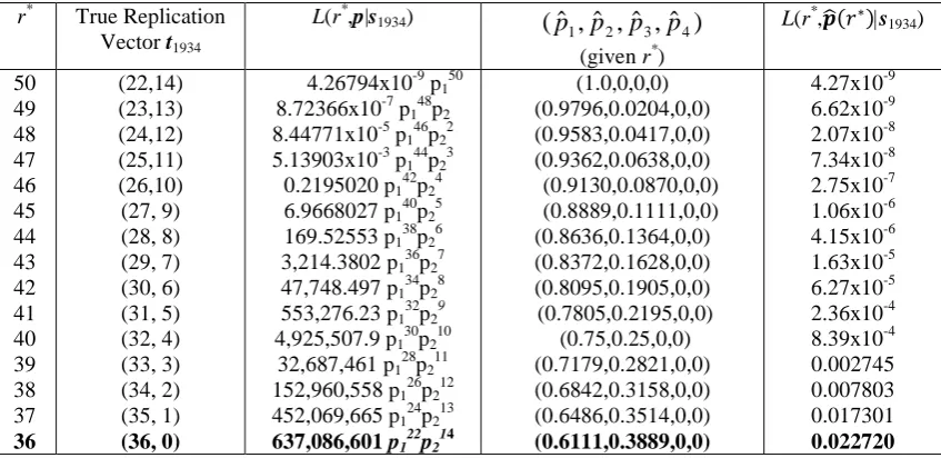
As a second example for birth year 1934 of the 1991 dataset and for r*=36 the

likelihood function

L(r*,p|s1934) = 637,086,601 p122p214

and by using Lemma 1, we find that this is maximised over p at p1= 0.6111 and p2=

0.3889 and the rest of the pi 's are zero. In Section 5 we present in detail the results for

the year 1934 and some of the results for the year 1935 of the 1991 dataset in order to

show how the maximum likelihood method works.

5. REPLICATION AND OVERCOUNTING

In Section 6 we present the summary results for both datasets. But because it

is quite difficult to understand how the maximum likelihood method works, we

present first in detail how we obtained the results for two years. As stated before for i

≥ 1, pi is defined as the probability that an HIV positive individual who has had at

least one positive test recorded in the dataset has actually had exactly i positive HIV

tests recorded. Of course pi ≥ 0 for i ≥ 1 and

∑

∞

= =

1

1

i i

p .

In Tables 3 and 4 (see Appendix A) we present the results for the years 1934

and 1935 for the 1991 dataset. We give the results for all the possible outcomes for

the true replication vector tB, for a given value of r*, when we eliminate individuals

repeatedly recorded in the sample, where r* is the true number of individuals in the

sample (given in column one). The second column contains the true replication vector

or vectors corresponding to this r* and the third column the likelihood function

L(r*,p|sB) of r* and p given the observed data. Then the following column presents the

probabilities which maximise the likelihood function (for that value of r*). The last

column has the maximised likelihood function L(r*,𝒑�(𝑟∗)|sB) (given r*) .

For 1934 the observed replication vector is s1934 = (22,14). Hence the true

number of individuals is somewhere between 36 (if each of the doubletons correspond

exactly two distinct individuals). If r*=36 then the true replication vector after

individuals repeatedly counted have been eliminated is (36,0), if r*=37 then the true

replication vector is (35,1) and so on up to r*=50 when the true replication vector is

(22,14).

If r*=50 then the probability that all 50 individuals have had only one birth

date recorded is p150. The independent probability that there are 22 singleton birthdays

and 14 doubleton birthdays is calculated to be 4.26794x10-9 with the use of Theorem 1. So in that case

L(r*=50,p|s1934) = 4.26794x10-9p150

which has a maximum value of 4.26794x10-9at pˆ₁ =1,pˆ₂ = pˆ₃ =...=0.

In the second case of r*=49 we get the observed replication vector precisely

when exactly one individual has had two recorded positive tests and this individual

has a distinct birthday from everyone else. The rest of the individuals must have had

exactly one test. So after the elimination of the double counting, the true replication

vector is (23,13). The probability of 49 randomly chosen individuals giving rise to the

true replication vector of birth dates is calculated using Theorem 1 to be 3.7929x10-8. The probability that exactly one out of the 23 singleton birth dates corresponds to an

individual who has had two recorded HIV tests and everyone else has had exactly one

is 23p148p2. So the likelihood function is:

L(r*=49,p|s1934) = 3.7929x10-8 x 23 p148p2 = 8.72366x10-7p148p2.

By Lemma 1, this has a maximum value of 6.61714x10-9, when 0

... ˆ ˆ , 0204 . 0 ˆ , 9796 . 0

ˆ₁ = p₂ = p₃ = p₄ = =

p .

In the same way, for r*=48, the probability of 48 randomly chosen individuals,

each counted once giving rise to the replication vector (24,12) is 3.06076x10-7. But in order to get this replication vector out of the original data, we must have exactly two

individuals out of the 24 singleton birth dates corresponding to an individual who has

had two recorded tests and all the other 46 individuals in the sample having had just

one recorded test. The likelihood is then:

L(r* =48, p|s1934) = 3.06076x10-7

! 2

24 .

23 _p

146p22 = 8.44771x10-5p146p22.

The maximum value for this function is 2.07052x10-8 when

0 ... ˆ ˆ , 0417 . 0 ˆ , 9583 . 0

ˆ₁ = p₂ = p₃ = p₄ = =

Finally after calculating all the possible outcomes for the true replication

vector and the respective maximum likelihood functions, we estimate that for the year

1934 in the 1991 dataset, there were 14 individuals reported exactly twice and the rest

of the individuals were reported exactly once. So the corresponding true replication

vector would be t1=36, t2=t3=t4=0, and the maximised likelihood function was 0.0227

for ˆp₁ =0.6111,ˆp₂ =0.3889,pˆ₃ = ˆp₄ =...=0.

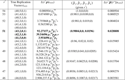
For the birth year 1935 the calculations are more complicated because of the

presence of a four-tuple in the observed data. For example we can see that if the true

value of r*=53, then we have two possible true replication vectors corresponding to

the same value of r*. That means that the maximum likelihood function for r*=53 is

L(r* =53,p|s1935) = 41P(41,4,0,1) x p152p2 + 3P(40,5,1,0) x p152p2 = 0.0750 p152p2, the

maximised value of which is calculated to be 0.000525, when the estimated

probabilities are pˆ₁ =0.9811,pˆ₂ =0.0189,pˆ₃ = pˆ₄ =...=0 . Here the notation

P(t1,t2,t3…, tr) denotes the probability of observing the birth date replication vector tB

= (t1,t2,t3…, tr) if there are r*=

∑

=

r

i i it

1

distinct individuals in the sample and each has

only one recorded HIV test.

It is obvious from the next cases for the year 1935 that we can have different

replication vectors corresponding to the same value of r* and even different factors

corresponding to the same replication vectors or vice versa. Different factors

corresponding to the same true replication vector occurs for r*=47 where both

p141p25p3 and p142p24p4 correspond to the true replication vector (45,1,0,0). We

presented the situation of different replication vectors corresponding to the same

value of r* for r*=53.

Finally after calculating all the possible outcomes for the true replication

vector and the respective maximum likelihood functions, we came to the conclusion

that for 1935, it is most likely that r*=51 (and hence there was one person counted

four times and fifty one people counted exactly once). The true replication vector was

estimated as (t1,t2,t3,t4) = (41,5,0,0) and the maximised likelihood for this vector was

0.0288, which occurred when pˆ₁ =0.9804, pˆ₂ =0.0, pˆ₃ =0.0, pˆ₄ =0.0196,

0 ... ˆ

ˆ₅ = p₆ = =

p . As the number of observations in a year becomes even larger the

6. SUMMARY RESULTS

We used two different programs for these calculations. Two versions were

written, one in Fortran, one in C. For each possible value of r*, the first program

calculated all the possibilities for the true replication vector TB= (T1, T2, …T11) giving

the same value for r* and the relative probabilities for those vectors. Then for each

value of r*, the second program calculated the likelihood function L(r*,p|sB) using the

probabilities from the first program, and maximised it with respect to p, calculated the

maximising value pˆ and the partially maximised likelihood function L(r*,pˆ(r*)|sB)

(given r*). Further details of the programs and algorithm used are given in Sfikas

[24].

We present for the 1991 dataset, wherever it is possible, all the possible

outcomes for the replication vector together with the respective calculated maximum

likelihood estimators. For this dataset for the birth years 1934-1941, pˆ_i was always

zero for i ≥ 5 so we give only pˆ₁, pˆ₂, pˆ₃ and pˆ₄. For the birth years and

1942-1944, pˆ was always zero for _i i ≥ 7, so we give only pˆ₁, pˆ₂, pˆ₃, pˆ₄, pˆ₅ and pˆ₆. For

the 1994 dataset it was difficult to give as much detail for the vast majority of birth

years, due to the large number of HIV positive records in the observed data and the

large size of the subsequent possible outcomes. So for this dataset we just present 𝑟_�∗

and 𝒑�(𝑟�∗) _{and the maximised likelihood function L(𝑟�}∗_,𝒑�(_𝑟�∗)_{|sB). As for this dataset}

i p ˆ

was always zero for i ≥ 12 we give only pˆ₁,pˆ₂,...,pˆ₁₀and pˆ₁₁.

In Tables 5 and 6 we present the results for the 1991 dataset and in Table 7 the

results for the 1994 dataset. The first column of Table 5 gives the year of birth and the

second one all the possible outcomes for the true number r* of distinct individuals in

the sample born during that year. The third column shows for each possible outcome

for r the true replication vector (or vectors) that correspond to the specific value of r.

The fourth column gives the likelihood function for each value of r and p. The

maximised likelihood function is given in the last column. For each year we also give

the values 𝑟_�∗ _{of r}*

and (pˆ₁,pˆ₂,pˆ₃,pˆ₄)that maximise the likelihood function.

We should also mention that for the years 1929-1933 of the 1991 database the

results were presented in full by Greenhalgh, Doyle and Mortimer [22]. So they are

which could not be analytically presented in full due to their length.

In the 1991 dataset we estimated that there was some replication in five out of

the sixteen birth years for which we had data. The years where replication was

estimated to be present were: 1931, 1934, 1935, 1943 and 1944. The amount of

replication that we estimated to be present was 37 records out of 1,097 which is

equivalent to a 3.37% proportion of replication.

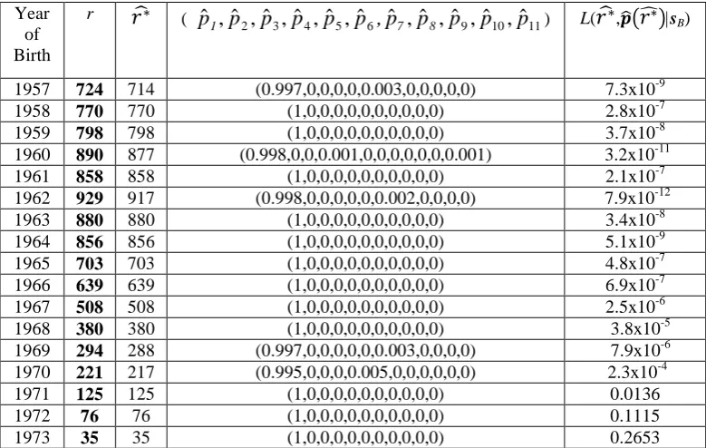
For the 1994 dataset the results are summarised in Table 7. The first column

again gives the year of birth of the individuals found HIV positive, the second column

shows the observed total number of HIV positive records in this birth year and the

third column the estimated number of distinct individuals by using the maximum

likelihood method. The replication is the “observed number” r minus the “estimated

number” 𝑟�∗. Column four gives us the probabilities which maximise our likelihood

estimator. Further details could not be presented due to lack of space. Finally, the last

column gives the maximised likelihood estimator (with the estimated 𝑟�∗ as shown in

the third column).

We found that there was replication present in 16 years out of the 64 years

examined. The amount of replication present in this dataset was 100 records out of a

sample of 17,272 which is the actual total number of individuals tested according to

our research after we get rid of the replication present. This gives us a replication of

0.58% of the total number of distinct individuals present. Thus the replication found

in the 1994 dataset is less than one fifth of the one found in the 1991 dataset. This can

be attributed to the fact that the PHLS was able to eliminate much but not all of the

replication when collecting the 1994 dataset, by improving their methods of

identifying repeatedly counted individuals.

Hence we have obtained a point estimate of the percentage replication in the

PHLS HIV test data. However point estimates by themselves are of limited value and

it is more useful to have some indication of the amount of uncertainty associated with

these estimates. To do this we calculated 95% bootstrap confidence intervals based on

the percentile method. However because the bootstrap distribution of the estimated

percentage amount of replication was skew, rather than use the simple percentile

method we use a more appropriate method which reflected an adjusted version of the

bootstrap distribution about the estimated value [25]. This is sometimes called the

observed individual records, we estimated𝑟�∗, the number of distinct individuals in the sample, as above, and 𝒑�(𝑟�∗), the probability distribution of the number of reported HIV tests that an individual has had. Next we took a random bootstrap sample of 𝑟�∗

independent individuals whose birth dates were chosen at random and each of whom

was independently assigned a number of HIV tests according to the distribution

𝒑�(𝑟_�∗_{). Then for this simulated observed replication vector the maximum likelihood} method was again applied to estimate the amount of replication corresponding to that

observed replication vector and the percentage replication calculated. This was

repeated with 100 random bootstrap samples to give a distribution of the amount of

replication in a sample and a bootstrap confidence interval calculated as follows:

Suppose that η denotes the true percentage replication in our sample. For each

bootstrap sample we calculate η*−ηˆ

where η*is the estimated percentage replication

in the bootstrap sample and ηˆis the estimated percentage replication. From these we

find the empirical values δL and δU such that 2.5% of the adjusted observations lie

below δL and 2.5% lie above δU. Hence we deduce the 95% bootstrap confidence

interval for the true percentage replication η as

(ηˆ−δU,ηˆ−δL).

The estimated percentage replication for the PHLS 1991 dataset is shown in

Table 8 together with the associated 95% bootstrap confidence intervals. These were

calculated using our C program. From this table it is clear that the birth years with the

wider confidence intervals tend to have relatively high estimated probabilities of an

individual having two or more HIV tests. Note that the point estimates for the

percentage replication always lie within the corresponding 95% bootstrap confidence

interval supporting the validity of the method. From the confidence intervals we

deduce that a 95% confidence interval for the overall amount of replication in this

dataset is (0.98%,11.83%).

Using the C program, we used the parametric bootstrap method to generate

95% bootstrap confidence intervals for the 1994 dataset. These are shown in Table 9.

The birth years with the narrower confidence intervals again tend to have relatively

low estimated probabilities of an individual having two or more HIV tests and

relatively high numbers of birth records, thus relatively high numbers of individuals.

This is what would be expected. Again point estimates for the percentage replication

confidence intervals we deduce that a 95% confidence interval for the overall amount

of replication in this dataset is (0%,2.64%).

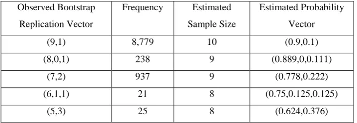
7. VALIDATION OF THE METHOD

We take a simple example to test the validity of the method. We take the artificial

replication vector (9,1) as an example so that nine individuals have had exactly one

HIV test and one individual has had exactly two HIV tests. We allocate the birth dates

at random to each individual to construct the observed birth record replication vector

then use the maximum likelihood method to estimate the amount of replication in this

vector. The process was repeated 10,000 times with results as shown in Table 10.

We had to perform the simulation a large number of times to get an accurate

distribution for the observed birth record replication vector and the program took a

long time to run. Hence we had to choose a small true number of individuals (10).

Consequently the resulting bootstrap confidence intervals were quite wide.

Nonetheless the method is validated quite well. In 87.8% of cases the sample size was

estimated correctly and in a further 11.7% of cases it was just one out. In the 87.8% of

cases where the sample size was estimated correctly the probability vector was also

estimated correctly.

The 95% bootstrap confidence intervals associated with the observed bootstrap

replication vector were typically quite large. For example for the replication vector

(9,1) this was (0%,31.75%) and for (8,0,1) it was (0%,66.67%). Note that the

simulations to calculate the observed bootstrap replication vector were conditional on

there being exactly one individual in the dataset who had had exactly two reported

HIV tests and that the simulations to calculate the 95% bootstrap confidence intervals

were conditional on both the estimated sample size and the number of reported HIV

tests that an individual had had following the estimated probability distribution.

8. DISCUSSION

We were given two datasets by the PHLS AIDS Surveillance Centre,

containing only numbers of repeated birth dates by year of birth for individuals whose

HIV positive test had been reported. As, for various reasons, many people with HIV

these datasets. Our aim was to quantify the replication. A maximum likelihood

estimation method was used along with the parametric bootstrap method to construct

the corresponding 95% confidence intervals. We estimated that the replication

present in the 1991 dataset was 3.37% (95% confidence interval (0.98%,11.83%)) and

for the 1994 dataset 0.58% (0%,2.64%). We noted before that we expected the

replication to be smaller in the 1994 database because both the current and

retrospective rates of inclusion in records of surname Soundex code had improved by

that date. This made for more efficient elimination of replicate reports of the same

individual from the national database than had been possible earlier. This

improvement must be offset by people presenting for testing under different names, a

problem that can only increase over time. Of course, the accuracy of the estimation

process relies on the available information, and in this sense any estimate of

replication would provide a minimum value for the true replication. Underlinking may

particularly affect certain subgroups, such as women who are, through marriage, more

likely than men to change their surname, and thus its Soundex code, and patients of

foreign origin for whom surname may be less consistently distinguished from

forename than is the case for those born in the UK. This would tend to distort the

view of the epidemic in the UK. Female patients and patients from abroad with

heterosexually acquired HIV may historically have been differentially

overrepresented in the database due to overlinking, but this differential contribution

has yet to be estimated.

In 2011 there were an estimated 6,280 people in the UK newly diagnosed as

HIV infected [26]. In view of the numbers and problems already described it is

obvious that there will continue to be underlinking of reports which in fact relate to

the same individual.

The work presented here ignores the possible inconsistencies in the recording

of dates of birth for individuals reported more than once; the presence of these will

lead to unquantifiable numbers of unrecognised repeat records. Those making the

reports were fully aware of the importance of accuracy and double entry was used at

the PHLS AIDS Surveillance Centre with the aim of minimising such errors.

A preliminary version of the method used in this paper was used in [22] to

analyse the amount of replication in five birth years from the 1991 dataset where the

sample sizes were very small. The current paper very substantially extends this work

substantially increased and the method is much more complex. It also extends the

work in [22] by calculation of bootstrap confidence intervals for the percentage

replication.

Importantly for the 1991 dataset, the years where we found replication by the

method used here were the same as the ones identified by the matching pairs method

[15]. The same conclusion is arrived at by two distinct methods, re-inforcing our

confidence in the results.

REFERENCES

1. Anderson RM, May RM. Infectious Diseases of Humans: Dynamics and Control. Oxford University Press: Oxford, 1991.

2. Benenson S. Control of Communicable Diseases in Man. 16th ed., American Public Health Association: Washington, D.C., 1990.

3. Doyle MT. Modelling Some Aspects of the AIDS Pandemic. Ph.D. thesis, University of Strathclyde: Glasgow, UK, 1994.

4. Chan, M., Sidibé, M. And Lake, A. Global HIV/AIDS response – Epidemic update and health sector progress towards Universal Access – Progress Report 2011, Joint World Health Organisation, UNAIDS, UNICEF Report, World Health Organisation, Geneva, Switzerland, 2011.

5. Longini IM, Clark WS, Byers RH, Ward JW, Darrow WW, Lemp GF, Hethcote HW. Statistical analysis of the stages of HIV infection using a Markov model. Statistics in Medicine 1989; 8:831-843.

6. Evans G, Howitt DJ, Mortimer J. Surveillance of HIV infection and AIDS in the U.K.: an overview from the PHLS AIDS Centre. PHLS Microbiology Digest 1993; 10:141-143.

7. Mortimer J, Salathiel JA. ‘Soundex’ codes of surnames provide confidentiality and accuracy in a national HIV database. Communicable Disease Report 1995; 5:183-186.

8. McHenry A, Macdonald N, Sinka K, Mortimer J, Evans B. National assessment of

prevalent diagnosed HIV infections, Communicable Disease and Public Health

2000;3:277-281.

9. Rice BD, Delpech DC, Chadborn TR, Elford J. Loss to follow-up among adults attending Human Immunodeficiency Virus Services in England, Wales and Northern Ireland,

Sexually Transmitted Diseases, 2011:38:685-690.

10.Larsen SO. Estimation of the number of people in a register from the number of birthdates. Statistics in Medicine 1994; 13:177-183.

11.Acheson ED. Medical Record Linkage. Oxford University Press: London, 1976.

12.Newcombe HB. Handbook of Record Linkage Methods for Health and Statistical Studies, Administration and Business. Oxford University Press: London, 1988.

13.Jaro MA. Probabilistic linkage of large public health data files. Statistics in Medicine

1995; 14:491-498.

14.Shevenko IP, Lynch JT, Mattie AS, Reed-Fourquet LI. Verification of information in a large medical database using linkages with an external database. Statistics in Medicine

1995; 14:511-530.

15.Greenhalgh D, Doyle MT. A test to detect replication in HIV serological data labelled by birthdate based on the number of matching pairs in a sample. Statistics in Medicine 1999;

16.Blakely T, Salmond C. Probabilistic record linkage and a method to calculate the positive predictive value, International Journal of Epidemiology 2002;31:1246-1252.

17.Elmagarid AK, Ipeiritos PG, Verykios VS. Duplicate record detection: a survey. IEEE Transactions on Knowledge and Data Engineering 2007;19:1-16.

18.Ades AE, Walker J, Botting B, Parker S, Cubitt, D, Jones R. Effect of the worldwide epidemic on HIV prevalence in the United Kingdom: record linkage in anonymous neonatal seroprevalence surveys. AIDS 1999;13:2437-2443.

19.Goubar A, Ades AE, De Angelis D, McGarrigle CA, Mercer CH, Tookey PA, Fenton K, Gill ON. Estimates of human immunodeficiency virus prevalence and proportion diagnosed based on Bayesian multiparameter synthesis of surveillance data. J. R. Statist. Soc. A 2008;171:541-580.

20.Presanis AM, De Angelis D, Goubar A, Gill ON, Ades AE. Bayesian evidence synthesis for a transmission dynamic model for HIV among men who have sex with men.

Biostatistics 2011;12:666-681.

21.Doyle MT, Greenhalgh D, Mortimer J. Three statistical tests for detecting overcounting of individuals in serological test data, Applied Stochastic Models and Data Analysis. 1998; 13:307-314.

22.Greenhalgh D, Doyle MT, Mortimer J. A partial ranking method for identifying repeated inclusion of individuals in anonymised HIV infection reports. Biometrics. 1999; 55 :165-173

23.Day NE. The incidence and prevalence of AIDS and other severe HIV disease in England and Wales for 1992-1997. Communicable Disease Report. 1993; 3(Supplement 1) :S1-S17.

24.Sfikas N. Mathematical Models for Vaccination Programs and Statistical Analysis of Infectious Diseases of Humans. Ph.D. thesis, University of Strathclyde: Glasgow, UK, 1999.

25.Efron B, Tibshirani RJ. An Introduction to the Bootstrap. Chapman and Hall: New York, 1993.

APPENDIX A.

Year of Birth

r S1 S2 S3 S4 S5 S6

1929 28 26 1 - - - -

1930 25 23 1 - - - -

1931 26 19 2 1 - - -

1932* 27 23 2 - - - -

1933 44 38 3 - - - -

1934 50 22 14 - - - -

1935 54 40 5 - 1 - -

1936* 52 48 2 - - - -

1937 68 57 4 1 - - -

1938 78 66 6 - - - -

1939 99 67 13 2 - - -

1940* 87 71 8 - - - -

1941 83 63 10 - - - -

1942 124 86 13 4 - - -

1943 113 69 17 2 1 - -

1944* 176 104 24 6 - - 1

Year of Birth

r S1 S2 S3 S4 S5 S6 S7 S8 S9 S10 S11

1901 0 - - - -

1902 0 - - - -

1903 1 1 - - - -

1904* 0 - - - -

1905 2 2 - - - -

1906 0 - - - -

1907 0 - - - -

1908* 1 1 - - - -

1909 0 - - - -

1910 0 - - - -

1911 2 2 - - - -

1912* 4 4 - - - -

1913 5 5 - - - -

1914 10 10 - - - -

1915 5 5 - - - -

1916* 4 2 1 - - - -

1917 7 5 1 - - - -

1918 6 6 - - - -

1919 10 8 1 - - - -

1920* 6 6 - - - -

1921 3 3 - - - -

1922 11 7 2 - - - -

1923 13 13 - - - -

1924* 19 17 1 - - - -

1925 33 28 1 1 - - - -

1926 20 17 - 1 - - - -

1927 24 22 1 - - - -

1928* 30 26 2 - - - -

1929 41 39 1 - - - -

1930 43 35 4 - - - -

1931 52 37 6 1 - - - -

1932* 59 51 4 - - - -

1933 74 68 3 - - - -

1934 82 60 8 2 - - - -

1935 78 59 8 1 - - - -

1936* 95 69 10 2 - - - -

1937 118 86 16 - - - -

1938 129 96 12 3 - - - -

1939 156 94 25 4 - - - -

1940* 143 106 17 1 - - - -

1941 149 105 19 2 - - - -

1942 212 101 43 7 1 - - - -

1943 202 115 28 9 1 - - - -

1944* 280 127 49 14 2 1 - - - -

1945 279 118 55 11 2 2 - - - -

1946 320 130 56 18 6 - - - -

1947 411 133 69 35 6 1 1 - - - - -

1948* 392 128 66 27 9 3 - - - -

1949 418 150 66 29 11 1 - - - -

1950 430 131 68 36 10 3 - - - -

1951 444 137 78 33 6 3 1 1 - - - -

1952* 515 131 91 41 13 3 2 - - - - -

1953 485 133 75 35 11 6 1 - 1 1 - -

1954 591 110 78 53 28 7 2 1 - - - -

1955 624 88 104 57 24 11 1 - - - - -

Year of Birth

r S1 S2 S3 S4 S5 S6 S7 S8 S9 S10 S11

1957 724 103 99 57 30 15 2 4 1 1 - -

1958 770 84 107 62 40 15 5 3 - - - -

1959 798 86 91 75 37 18 4 5 1 - - -

1960* 890 87 92 71 37 25 8 7 2 1 - 1

1961 858 79 96 72 48 19 9 2 2 - - -

1962 929 68 107 55 47 29 13 4 3 1 1 -

1963 880 82 80 75 47 25 12 4 - - - -

1964* 856 80 87 76 42 18 12 5 - 1 - -

1965 703 107 92 71 28 9 7 - - - - -

1966 639 109 96 52 22 15 2 1 - - - -

1967 508 114 88 38 16 8 - - - -

1968* 380 123 68 24 11 1 - - - -

1969 294 112 63 12 2 1 - 1 - - - -

1970 221 107 41 9 - 1 - - - -

1971 125 92 12 3 - - - -

1972* 76 62 7 - - - -

1973 35 31 2 - - - -

r* True Replication Vector t1934

L(r*,p|s1934) (ˆ , ˆ , ˆ , ˆ ) 4 3 2

1 p p p

p

(given r*)

L(r*,𝒑�(𝑟∗)|s1934)

50 49 48 47 46 45 44 43 42 41 40 39 38 37 36 (22,14) (23,13) (24,12) (25,11) (26,10) (27, 9) (28, 8) (29, 7) (30, 6) (31, 5) (32, 4) (33, 3) (34, 2) (35, 1) (36, 0)

4.26794x10-9 p150

8.72366x10-7 p148p2

8.44771x10-5 p146p22

5.13903x10-3 p144p23

0.2195020 p142p24

6.9668027 p140p25

169.52553 p138p26

3,214.3802 p136p27

47,748.497 p134p28

553,276.23 p132p29

4,925,507.9 p130p210

32,687,461 p1 28

p2 11

152,960,558 p126p212

452,069,665 p124p213 637,086,601 p122p214

(1.0,0,0,0) (0.9796,0.0204,0,0) (0.9583,0.0417,0,0) (0.9362,0.0638,0,0) (0.9130,0.0870,0,0) (0.8889,0.1111,0,0) (0.8636,0.1364,0,0) (0.8372,0.1628,0,0) (0.8095,0.1905,0,0) (0.7805,0.2195,0,0) (0.75,0.25,0,0) (0.7179,0.2821,0,0) (0.6842,0.3158,0,0) (0.6486,0.3514,0,0) (0.6111,0.3889,0,0) 4.27x10-9 6.62x10-9 2.07x10-8 7.34x10-8 2.75x10-7 1.06x10-6 4.15x10-6 1.63x10-5 6.27x10-5 2.36x10-4 8.39x10-4 0.002745 0.007803 0.017301 0.022720

r* True Replication Vector t1935

L(r*,p|s1935) (ˆ , ˆ , ˆ , ˆ ) 4 3 2 1 p p p

p

(given r*)

L(r*,𝒑�(𝑟∗)|s1935)

54 53 52 51 50 49 48 47 46 (40,5,0,1) (41,4,0,1) (40,5,1,0) (42,3,0,1) (41,4,1,0) (40,6,0,0) (43,2,0,1) (42,3,1,0) (41,5,0,0) (44,1,0,1) (43,2,1,0) (42,4,0,0) (45,0,0,1) (44,1,1,0) (43,3,0,0) (45,0,1,0) (44,2,0,0) (45,1,0,0) (46,0,0,0)

0.000504 p1 54

0.074989 p152p2

3.755868 p150p22+

0.563380 p1 51

p3 92.27157 p148p23+ 39.54496 p149p2p3+

3.954496 p150p4 1,226.411 p146p24+

1,132.072 p147p22p3+

283.0179 p148p2p4

8,546.151 p1 44

p2 5

+ 16,528.24 p145p23p3+

8,264.122 p146p22p4

24,623.71 p142p26+

123,118.6 p1 43

p2 4

p3+

123,118.6 p144p23p4

374,485.6 p141p25p3+

936,214.0 p142p24p4

2,908,237.5 p140p25p4

(1.0,0,0,0) (0.9811,0.0189,0,0)

(0.981,0, 0.019,0)

(0.9804,0,0, 0.0196)

(0.96, 0.02,0, 0.02)

(0.9385,0.041,0,0.0205)

(0.9167, 0.0625,0, 0.0208)

(0.8936, 0.0851,0, 0.0213) (0.8696, 0.1087,0, 0.0217)

0.000504 0.000525 0.004024 0.028808 0.015985 0.015424 0.013704 0.009279 0.003581

Year of Birth

r* True Replication

Vector tB

L(r*,p|sB) L(r*,𝒑�(𝑟∗)|sB)

1934 50 49 48 47 46 45 44 43 42 41 40 39 38 37 36 (22,14) (23,13) (24,12) (25,11) (26,10) (27, 9) (28, 8) (29, 7) (30, 6) (31, 5) (32, 4) (33, 3) (34, 2) (35, 1) (36, 0)

4.26794x10-9 p150

8.72366x10-7 p148p2

8.4477x10-5 p146p22

5.1390x10-3 p144p23

0.2195020 p142p24

6.9668027 p140p25

169.52553 p138p26

3,214.3802 p136p27

47,748.497 p134p28

553,276.23 p1 32

p2 9

4,925,507.9 p130p210

32,687,461 p128p211

152,960,558 p126p212

452,069,665 p124p213 637,086,601 p122p214

4.27x10-9 6.62x10-9 2.07x10-8 7.34x10-8 2.75x10-7 1.06x10-6 4.15x10-6 1.62x10-5 6.27x10-5 2.35x10-4 8.39x10-4 0.002745 0.007803 0.017301 0.022720 1934

𝒓�∗=36, ( 𝒑�𝟏,𝒑�𝟐,𝒑�𝟑,𝒑�𝟒) = (0.6111,0.3889,0,0)

1935 54 53 52 51 50 49 48 47 46 (40,5,0,1) (41,4,0,1) (40,5,1,0) (42,3,0,1) (41,4,1,0) (40,6,0,0) (43,2,0,1) (42,3,1,0) (41,5,0,0) (44,1,0,1) (43,2,1,0) (42,4,0,0) (45,0,0,1) (44,1,1,0) (43,3,0,0) (45,0,1,0) (44,2,0,0) (45,1,0,0) (46,0,0,0)

0.000504 p1 54

0.074989 p152p2

3.755868 p 1 50

p2 2

+

0.563380 p151p3 92.271572 p1

48

p2 3

+

39.54496 p149p2p3+ 3.954496 p150p4 1,226.4107 p146p24+

1,132.07 p147p22p3+

283.0179 p148p2p4

8,546.1509 p1 44

p2 5

+

16,528.24 p145p23p3+

8,264.122 p146p22p4

24,623.712 p1 42

p2 6

+

123,118.6 p143p24p3+

123,118.55 p144p23p4

374,485.6 p141p25p3+

936,214.0 p142p24p4

2,908,237.5 p140p25p4

0.000504 0.000525 0.004024 0.028808 0.015985 0.015424 0.013704 0.009279 0.003581

1935 𝒓�∗_{=51, (} 𝒑�_𝟏,𝒑�_𝟐,𝒑�_𝟑,𝒑�_{𝟒) = (0.98,0,0,0.02)}

1936 52

51 50

(48,2)

(49,1) (50,0)

0.181447 p152 5.094471 p150p2

36.56032 p1 48 p2 2 0.181447 0.037113 0.008244

1936 𝒓�∗_{=52, (} 𝒑�_𝟏,𝒑�_𝟐,𝒑�_𝟑,𝒑�_{𝟒) = (1,0,0,0)}

1937 68

67 66 65 64 63 62 (57,4,1) (58,3,1) (57,5,0) (59,2,1) (58,4,0) (60,1,1) (59,3,0) (61,0,1) (60,2,0) (61,1,0) (62,0,0)

0.045946 p168 3.452670 p166p2

96.7337 p1 64

p2 2

+

8.061138 p165p3

1,307.696 p162p23+

356.6443 p163p2p3

8,678.344 p1 60

p2 4

+

6,008.085 p161p22p3

22,843.24 p158p25+

45,686.48 p159p23p3

132,345.7 p1 57 p2 4 p3 0.045946 0.019100 0.045276 0.012565 0.005448 0.001769 0.000306

Year of Birth

r* True Replication

Vector tB

L(r*,p|sB) L(r*,𝒑�(𝑟∗)|sB)

1938 78

77 76 75 74 73 72 (66,6) (67,5) (68,4) (69,3) (70,2) (71,1) (72,0)

0.104460 p178 5.865815 p176p2

139.02744 p174p22

1,780.52689 p172p23

12,997.8467 p170p24

51,288.8067 p168p25

85,481.2751 p166p26

0.104460 0.028208 0.013381 0.006029 0.002269 0.000621 0.000092

1938 𝒓�∗_{=78, (} 𝒑�

𝟏,𝒑�𝟐,𝒑�𝟑,𝒑�𝟒) = (1,0,0,0)

1939 99

98 97 96 95 94 93 92 91 90 89 88 87 86 85 84 83 82 (67,13,2) (68,12,2) (67,14,1) (69,11,2) (68,13,1) (67,15,0) (70,10,2) (69,12,1) (68,14,0) (71,9,2) (70,11,1) (69,13,0) (72,8,2) (71,10,1) (70,12,0) (73,7,2) (72,9,1) (71,11,0) (74,6,2) (73,8,1) (72,10,0) (75,5,2) (74,7,1) (73,9,0) (76,4,2) (75,6,1) (74,8,0) (77,3,2) (76,5,1) (75,7,0) (78,2,2) (77,4,1) (76,6,0) (79,1,2) (78,3,1) (77,5,0) (80,0,2) (79,2,1) (78,4,0) (80,1,1) (79,3,0) (81,0,1) (80,2,0) (81,1,0) (82,0,0)

0.0100108 p1 99

1.4025257 p1 97

p2

96.02954 p195p22+

1.6495871 p196p3

4,367.806 p193p23+

198.6307 p194p2p3

99,506.85 p191p24+

11,044.95 p192p22p3

70.8010 p193p32

1,999,201 p189p25+

377,208 p1 90

p2 3

p3+

7,072.65 p191p2p32

30,410,620 p187p26+

8,861,372 p188p24p3+

329,555 p1 89

p2 2

p3 2

357,270,106 p185p27+

1.518x108 p186p25p3+

9,485,047 p187p23p32

3.274x109 p183p28+

1.957x109 p184p26p3+

1.882x108 p185p24p32

2.344x1010 p181p29+

1.93x1010 p182p27p3+

2.717x109 p183p25p32

1.303x1011 p179p210+

1.47x1011 p180p28p3+

2.938x1010 p1 81

p2 6

p3 2

5.538x1011 p177p211+

8.57x1011 p178p29p3+

2.41x1011 p179p27p32

1.749x1012 p175p212+

3.78x1012 p176p210p3+

1.50x1012 p177p28p32

3.902x1012 p173p213+

1.22x1013 p174p211p3+

6.99x1012 p175p29p32

5.615x1012 p171p214+

2.73x1013 p172p212p3+

2.37x1013 p1 73

p2 10

p3 2

4.276x1012 p169p215+

3.80x1013 p170p213p3+

5.56x1013 p171p211p32

2.48x1013 p168p214p3+

8.05x1013 p169p212p32

5.45x1013 p167p213p32

Year of Birth

r* True Replication

Vector tB

L(r*,p|sB) L(r*,𝒑�(𝑟∗)|sB)

1939 𝒓�∗_{=99, (} 𝒑�_𝟏,𝒑�_𝟐,𝒑�_𝟑,𝒑�_{𝟒) = (1,0,0,0)}

1940 87

86 85 84 83 82 81 80 79 (71,8) (72,7) (73,6) (74,5) (75,4) (76,3) (77,2) (78,1) (79,0)

0.083757 p187 5.637743 p185p2

167.9523 p183p22

2,892.732 p181p23

31,510.11 p179p24

222,317.1 p177p25

992,293.6 p175p26

2,562,112 p1 73

p2 7

2,930,416 p171p28

0.083757 0.024258 0.012886 0.006926 0.003434 0.001475 0.000510 0.000126 0.000017

1940 𝒓�∗_{=87, (} 𝒑�_𝟏,𝒑�_𝟐,𝒑�_𝟑,𝒑�_{𝟒) = (1,0,0,0)}

1941 83

82 81 80 79 78 77 76 75 74 73 (63,10) (64,9) (65,8) (66,7) (67,6) (68,5) (69,4) (70,3) (71,2) (72,1) (73,0)

0.056044 p1 83 4.929215 p181p2

197.46915 p1 79

p2 2

4,745.7607 p177p23

75,783.866 p175p24

840,337.56 p173p25

6,553,914.7 p171p26

35,505,437.3 p169p27

127,889,651 p167p28

276,620,586 p165p29

272,882,184 p1 63 p2 10 0.056044 0.022250 0.016704 0.013190 0.010113 0.007219 0.004623 0.002539 0.001119 0.000312 0.000059

1941 𝒓�∗_{=83, (} 𝒑�_𝟏,𝒑�_𝟐,𝒑�_𝟑,𝒑�_{𝟒) = (1,0,0,0)}

Year of Birth

Observed

r

Estimated

𝑟�∗ ( pˆ1,pˆ2,pˆ3,pˆ4,pˆ5,pˆ6) L(𝑟�∗,𝒑��𝑟��∗ |sB)

1929 28 28 (1,0,0,0,0,0) 0.386

1930 25 25 (1,0,0,0,0,0) 0.379

1931 26 22 (0.864,0.091,0.045,0,0,0) 0.056

1932 27 27 (1,0,0,0,0,0) 0.170

1933 44 44 (1,0,0,0,0,0) 0.211

1942 124 124 (1,0,0,0,0,0) 0.007085

1943 113 102 (0.902,0.093,0.005,0,0,0) 0.001600 1944 176 171 (0.994,0,0,0,0,0.006) 0.001699