Time-delayed feedback control in astrodynamics

Time-delayed feedback control in astrodynamics

James D. Biggs

and Colin R. McInnes

In this paper we present time-delayed feedback control (TDFC) for the purpose of autonomously driving trajectories of nonlinear systems onto periodic orbits. As the gen-eration of periodic orbits is a major component of many problems in astrodynamics we propose this method as a useful tool in such applications. To motivate the use of this method we apply it to a number of well known problems in the astrodynamics literature. Firstly, TDFC is applied to control the chaotic attitude motion of an asymmetric satellite in an elliptical orbit. Secondly, we apply TDFC to the problem of maintaining a spacecraft in a periodic orbit about a body with large ellipticity (such as an asteroid) and finally, we apply TDFC to eliminate the drift between two satellites in low Earth orbits to ensure their relative motion is bounded.

1.

Introduction

Time-delayed feedback control (TDFC) is an efficient method for stabilizing unstable periodic orbits

embedded in chaotic attractors. TDFC was first proposed by Pyragus in 19921 _{as a simple and efficient}

method to control chaos in systems of ordinary differential equations. TDFC is based on applying a feedback

control that is proportional to the deviation of the current state of the system from its state one period in

the past, explicitly:

u(t) =−K(X(t)−X(t−τ)), (1)

where u(t) is the control, K is a gains matrix, X(t) is then-dimensional state vector and X(t−τ) is the

state one period in the past with period τ. The fundamental difference between the control (1) and that

of a Linear Quadratic Regulator (LQR)2 _{used for practical orbital control is that TDFC tracks a delayed}

trajectory rather than a reference trajectory. This is fundamentally different as the delayed trajectory can

evolve continuously over time (unlike a pre-specified reference trajectory in LQR). The authors propose this

method not as an alternative to LQR but as a highly autonomous control (requiring only a pre-specified

∗_{[email protected], Lecturer, Advanced Space Concepts Laboratory, Department of Mechanical Engineering,}

Uni-versity of Strathclyde, Glasgow.

†_{[email protected], member AIAA, Professor, Advanced Space Concepts Laboratory, Department of Mechanical}

period) that can be used for stabilizing unstable periodic orbits embedded in chaotic attractors and for

bounding the motion of unstable trajectories. Furthermore, TDFC has been successful in many applications,

for example, in the stabilization of laser coherent modes,3, 4 _{control of heart conductivity,}5 _{and to control}

systems with friction.6 _{The main advantages of this method are that is does not require a reference orbit for}

its implementation and can therefore be applied to systems without a priori knowledge of their dynamics.

However, it does require that the period of the orbit be specified a priori and once this is specified the

target orbit is essentially chosen. To the authors knowledge the only application of TDFC to a problem in

orbital dynamics is in the generation of periodic reference trajectories above the ecliptic plane in the solar

sail elliptic three-body problem7and to the stabilization of halo orbits.8

The general problem considered in this paper is to apply TDFC (1) to a nonlinear system of the form:

˙

X(t) =f(X(t)) +Bu(t), (2)

such that it drives X(t) onto a periodic orbit of some pre-specified period τ. Here B is a constant n×m

matrix wherem is the number of controls and a ‘dot’ denotes differentiation w.r.t time. Defining the error

in the period by the functionalke(t)k=kX(t)−X(t−τ)kthe general objective is to minimizeke(t)kover

the time intervalt∈[0, T] whereT is the final time. Ifke(t)k= 0 att=T thenu(t) = 0 and the final state

is a natural periodic orbit of the nonlinear system (2).

Traditionally, TDFC has been applied to control chaos in low-dimensional systems of ordinary differential

equations. However, it is somewhat surprising that this method has not found its way into mainstream

astrodynamic applications considering the large number of chaotic phenomena that exist.9, 10 _{This is perhaps}

due to an incorrect claim that the method has an inherent limitation known as the odd number limitation.11, 12

The odd number limitation asserts that TDFC cannot stabilize an unstable periodic orbit with an odd number

of real positive Floquet multipliers greater than 1. However, recently this limitation has been refuted in a

number of papers.13–15 _{These findings open up the possibility for TDFC to be used in trajectory tracking}

applications and to stabilize periodic orbits that are not necessarily embedded in chaotic attractors. To

this end we illustrate how this method has the potential to be used in a variety of applications throughout

astrodynamics and practical orbit control. Firstly, we apply TDFC to the problem of controlling the chaotic

attitude motion of a satellite in an elliptical orbit. This application falls into the conventional use of TDFC

in that the target periodic orbit is embedded in a chaotic attractor.

The subsequent applications in this paper illustrate how TDFC may be used in a new setting, that is to

drive trajectories onto periodic orbits that are not embedded in chaotic attractors. These novel applications

involve using TDFC to bound the motion of unstable trajectories. Previously, TDFC has been applied to

stabilize an isolated periodic orbit i.e. not embedded in a chaotic attractor. Moreover, this was demonstrated

through the application of TDFC to stabilizing a halo orbit.8 _{However, this application is not considered}

even if initially close to a periodic orbit, the instability of the system dictates that the orbit will be quite far

from the initial periodic orbit after a full period. In addition, since halo orbits have large periods (around 6

months), the use of a time-lag of that magnitude in a feedback control law would be not be practical, given

the diverse issues that can arise over that time span. However, the applications in this paper are deemed

practical as their initial (near periodic) trajectory has a relatively large instability time scale with much

smaller natural periods of several hours. These applications involve using TDFC to (i) drive a spacecraft

autonomously onto a periodic orbit of pre-specified period about a body (asteroid) with large ellipticity and

(ii) to bound the relative motion between satellites in low Earth orbits.

Before proceeding to apply TDFC to these applications a gain matrixKmust be pre-specified for equation

(1). In the literature on chaos control the K matrix is generally tuned by trial and error. Furthermore,

the tuning of this gain matrix becomes increasingly complex with increases in the dimension of the system.

One such method for computing an optimal (adaptive) gain matrix for TDFC applied to high-dimensional

systems is illustrated in the appendix and in Biggs and McInnes.8

2.

Controlling the chaotic attitude motion of an asymmetric satellite in an

elliptical orbit

TDFC is traditionally used for stabilizing unstable periodic orbits embedded in chaotic attractors in

low-dimensional differential equations. Therefore, it is clear that TDFC has the potential to be applied to

a number of problems in astrodynamics that exhibit undesirable chaotic behavior.9, 10 _{To motivate this we}

apply TDFC to the problem of controlling the chaotic attitude motion of a spacecraft in an elliptic orbit

about a planetary body. A model of the chaotic planar attitude motion of a spacecraft in an elliptical orbit in

the gravitational field of the Earth with air drag and internal damping is used. In this example we use TDFC

to stabilize the tumbling attitude of the satellite to obtain predictable and verifiable attitude oscillations.

Assuming that the internal damping and the atmospheric resistance are proportional to the spacecraft’s

angular velocity and the square of angular velocity respectively, whose coefficients areγanc, then a simple

model that describes this motion is:10

¨

φ−2e_{1 +}sinv_e(1 + ˙_cosvϕ)+ Ksin 2φ 1 +ecosv +cφ˙

2₊ γφ˙

(1 +ecosv)2 = 0 (3)

where ˙φ = dφ_dv, φ¨ = d_dv2φ2, where φ is the libration angle in the orbital plane as measured from the local

vertical,eis the orbit eccentricity,v is the position angle of the spacecraft in its orbit as measured from the

perifocus andK = 3(B₂−_CA) where A, B and C are the principal moments of inertia. It is shown in10 _that

for larger eccentricity ethere is a greater domain of chaotic motion. For example withK = 0.75, γ= 0.05

and c = 0.04 chaotic motion exists for e > 0.137802. In the following example we illustrate how TDFC

controlu(t) we can recast the equations (3) into a form where TDFC can be applied:

˙

φ=s

˙

s=2e₁₊sin_ev_cos(1+_vs)−1+Ksin 2ecosφv−cs

2₋ γs

(1+ecosv)2 +u(t)

(4)

foru(t) = 0 we setK = 0.75, γ= 0.05, c= 0.04, e= 0.2 withϕ0= 0 and s0 = 1. This yields the chaotic

motion illustrated in the Figure 1.

-2 -1.5 -1 -0.5 0 0.5 1 1.5 2 -1.5

-1 -0.5 0 0.5 1 1.5 2

φ φ φ φ

d

φφφφ

/d

t

0 5 10 15 20 25 30 35 40 45 -2

-1.5 -1 -0.5 0 0.5 1 1.5 2

time

φφφφ

(i) (ii)

Figure 1. (i) Chaotic attractor of the libration angle (ii) Chaotic time-series of the libration angle (rads) in

non-dimensional time

We apply TDFC to induce a period of the attitude dynamics that is equal to the period of the orbit about

the central body, that is we setτ = 2π. The controlled trajectory is illustrated in Figure 2 and it can be

seen to converge to a periodic orbit of period 2π.

-2 -1.5 -1 -0.5 0 0.5 1 1.5 2 -1.5

-1 -0.5 0 0.5 1 1.5 2

φ φ φ φ

d

φφφφ

/d

t

Converges to a Periodic Orbit

0 5 10 15 20 25 30 35 40 45 -2

-1.5 -1 -0.5 0 0.5 1 1.5 2

time

φφφφ

(i) (ii)

Figure 2. (i) Phase space shows that the chaotic trajectory converges to a periodic orbit (ii) the chaotic time-series converges to a periodic time series

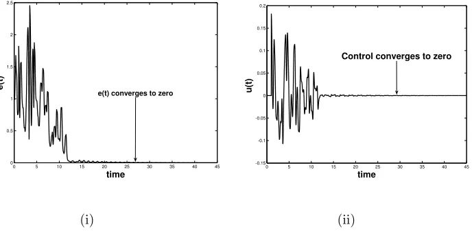
to zero. In addition as shown in Figure 3 (ii) the control converges to zero. This implies that the trajectory

has converged to a natural orbit embedded within the chaotic attractor. What is particularly useful about

0 5 10 15 20 25 30 35 40 45 0

0.5 1 1.5 2 2.5

e

(t

)

time

e(t) converges to zero

0 5 10 15 20 25 30 35 40 45 -0.15

-0.1 -0.05 0 0.05 0.1 0.15 0.2

time

u

(t

)

Control converges to zero

(i) (ii)

Figure 3. (i) error in the period of the trajectory converges to zero (ii) angular acceleration control

this approach is that extending the mission time will not require any active attitude control and therefore no

additional fuel will be required. Therefore, once the chaotic tumbling motion is stabilized to a predictable

oscillatory motion the pointing of sensors towards the Earth can be configured appropriately. The following

application concerns driving trajectories onto periodic orbits that are not embedded in chaotic attractors.

3.

Bounding the motion of a satellite about a body with large ellipticity

A characteristic of a spacecraft in orbit about a highly elliptical body is that the spacecraft orbit is highly

unstable leading often to orbit escape.16 _{Moreover, the spacecraft orbit can transition from a seemingly safe}

orbit into an impacting or escaping orbit within a few periods, see17 _{and references therein. In this section}

we investigate how TDFC can be used to counter this effect and maintain a spacecraft on a (stable) periodic

orbit about a highly elliptical body (such as an asteroid). A model of the spacecraft’s dynamics about a

uniformly rotating ellipsoid with constant density is used to define the spacecraft motion. The model used

is the restricted two-body problem with a simple ellipsoid potential as described in Koon. et al.18 _The

equations of motion for the massless satellite in a rotating Cartesian coordinate frame and appropriately

normalized18 _are:

¨

x−2 ˙y= ∂V ∂x

¨

y+ 2 ˙x= ∂V ∂y

(5)

where

V(x, y) = _√ 1

x2_+y2 +

1

2(x

2_+y2_{) +U}

22

U22= 3C22(x

2

−y2

) (x2_+y2₎5/2

The system (5) has one free parameter, the gravity field coefficientC22, commonly termed the “ellipticity”.

To illustrate the application of TDFC to this problem we take C22 = 0.052 which is the known value for

the asteroid Eros.16 _{We expand the state-space (5) to a system of first order differential equations and set}

u(t) =−BK[ux, uy]T _{whereB is the matrix}

B= 

 

0 0 1 0

0 0 0 1 

 

T

. (7)

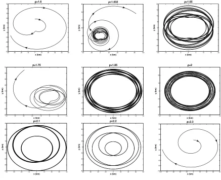
The equations (5) are therefore transformed into the form (2) and TDFC can be applied. Using the initial

conditionsx(0) = 0, y(0) = 1,x˙(0) =ρ,y˙(0) = 0 with values ofρbetween 0 and 3 we simulate a number of

trajectories over a 70 hour time interval. It is observed that for 0≤ρ < 1.6 and ρ > 2.3 the trajectory is

highly unstable. Several plots of different orbits over several days are given in Figure 4 within the interval

1.6≤ρ≤2.3. Note that in Figures 4 and 5 we have converted the non-dimensional units into real time and

length variables using the approximate data for Eros given in.16

-40 -30 -20 -10 0 10 20 30 40 50

-50 -40 -30 -20 -10 0 10 20 30 40 50 x (km) y ( k m ) ρ ρ ρ ρ=1.6

-40 -20 0 20 40 60 80 100

-40 -20 0 20 40 60 80 x (km) y ( k m ) ρ ρ ρ ρ=1.632

-20 -15 -10 -5 0 5 10 15 20

-20 -15 -10 -5 0 5 10 15 20 x (km) y ( k m ) ρ ρ ρ ρ=1.65

-50 -40 -30 -20 -10 0 10 20

-30 -20 -10 0 10 20 30 40 50 x (km) y ( k m ) ρ ρ ρ ρ=1.75

-20 -15 -10 -5 0 5 10 15 20

-20 -15 -10 -5 0 5 10 15 20 x (km) y ( k m ) ρ ρ ρ ρ=1.85

-30 -20 -10 0 10 20 30

-30 -20 -10 0 10 20 30 x (km) y ( k m ) ρ ρρ ρ=2

-40 -30 -20 -10 0 10 20 30 40

-40 -30 -20 -10 0 10 20 30 40 x (km) y ( k m ) ρ ρ ρ ρ=2.1

-80 -60 -40 -20 0 20 40 60 80

-80 -60 -40 -20 0 20 40 60 80 x (km) y ( k m ) ρ ρ ρ ρ=2.2

-100 -80 -60 -40 -20 0 20 40 60 80

-100 -80 -60 -40 -20 0 20 40 60 80 x (km) y ( k m ) ρ ρ ρ ρ=2.3

Figure 4. Uncontrolled trajectories for1.6≤ρ≤2.3.

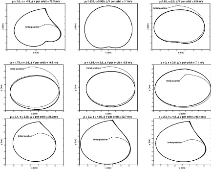
asteroid, namely forρ= 1.6,1.632,1.75,2.3 in Figure 4. In the following we apply TDFC to these trajectories

in order to induce stable periodic motions about the asteroid. Firstly, a Poincare sectionP is defined for

t > 0 such that {P : x= 0, y >0,x,˙ y˙}. Then the initial trajectory is defined as the curve in phase space

from the initial condition to the point where the trajectory intersects the Poincare section P. The delay

timeτ is then taken to be the time taken for the initial trajectory to intersect the Poincare section. TDFC is

then activated when the initial trajectory intersects the Poincare section. The TDFC controlled trajectories

are illustrated in Figure 5 with the average ∆V per orbit and delay times (non-dimensional units) specified.

-40 -30 -20 -10 0 10 20

-20 -10 0 10 20 30 40 50 x (km) y ( k m ) ρ ρ ρ

ρ = 1.6, ττττ = 4.3, ∆∆∆∆ V per orbit = 72.3 m/s

Initial position

-20 -15 -10 -5 0 5 10 15 20

-10 -5 0 5 10 15 20 x (km) y ( k m ) ρ ρ ρ

ρ=1.632, ττττ=3.065, ∆∆∆∆ V per orbit = 1.1m/s

-15 -10 -5 0 5 10 15 20

-15 -10 -5 0 5 10 15 20 x (km) y ( k m ) ρ ρ ρ

ρ=1.65, ττττ=2.8, ∆∆∆∆ V per orbit = 6.9 m/s

Initial position

-15 -10 -5 0 5 10 15 20

-15 -10 -5 0 5 10 15 20 x (km) y ( k m ) ρ ρ ρ

ρ = 1.75, ττττ = 2.6, ∆∆∆∆ V per orbit = 9.6 m/s

Initial position

-20 -15 -10 -5 0 5 10 15 20

-20 -15 -10 -5 0 5 10 15 20 x (km) y ( k m ) ρ ρ ρ

ρ = 1.85, ττττ = 2.9, ∆∆∆∆ V per orbit = 5.5 m/s

Initial position

-25 -20 -15 -10 -5 0 5 10 15 20

-25 -20 -15 -10 -5 0 5 10 15 20 25 30 x (km) y ( k m ) ρ ρ ρ

ρ = 2, ττττ = 3.5, ∆∆∆∆ V per orbit = 7.1 m/s

Initial position

-40 -30 -20 -10 0 10 20 30

-30 -20 -10 0 10 20 30 40 x (km) y ( k m ) ρ ρ ρ

ρ = 2.1, ττττ = 3.85, ∆∆∆∆ V per orbit = 31.2m/s

Initial position

-40 -30 -20 -10 0 10 20 30

-30 -20 -10 0 10 20 30 40 50 x (km) y ( k m ) ρ ρ ρ

ρ = 2.2, ττττ = 4.05, ∆∆∆∆ V per orbit = 52.7 m/s

Initial position

-50 -40 -30 -20 -10 0 10 20 30

-40 -30 -20 -10 0 10 20 30 40 50 60 x (km) y ( k m ) ρ ρ ρ

ρ = 2.3, ττττ = 4.2, ∆∆∆∆ V per orbit = 96.4 m/s

Initial position

Figure 5. TDFC implemented on the trajectories in Figure 4.

Figure 5 illustrates that TDFC bounds the motion of the spacecraft about the central ellipsoidal body. When

the initial trajectory is far from periodic i.e. ρ= 1.6,2.1,2.22.3 TDFC drives the trajectory onto a periodic

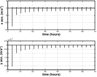
orbit but at the expense of high ∆V. Nevertheless, the average ∆V per orbit will reduce with increases

in mission time. This is illustrated in Figure 6 which shows the typical qualitative behavior of the TDFC

periodic orbit and then converge to a minimum. In this application it has been shown that TDFC can

0 10 20 30 40 50 60 70

-15 -10 -5 0 5x 10

-5

time (hours)

x

a

c

c

.

(m

/s

2)

0 10 20 30 40 50 60 70

-3 -2.5 -2 -1.5 -1 -0.5 0 0.5x 10

-3

time (hours)

y

a

c

c

.

(m

/s

2)

Figure 6. Typical TDFC: the initial control is large to close the orbit but converges to a small minimum over

time.

autonomously drive a spacecraft initially in an unstable or quasi-periodic orbit onto a periodic trajectory

about a central body with large ellipticity. This is useful in such an application as the gravity field coefficient

C22is often not known prior to orbit capture and therefore it is not possible to construct a suitable reference

trajectory a priori.

4.

Bounding satellite relative motion in low-Earth orbit

The idea of using several small, unconnected, satellites to form a large aperture has many advantages

as well as many technical challenges. The resolution of an imaging sensor is limited by the maximum

achievable aperture, so that a single aperture sensor is limited by its physical size. Larger apertures can be

achieved using a satellite formation whereby simply increasing the formation size will increase the aperture.

Therefore, formation flying can be used to obtain a much finer resolution than is possible for a single platform.

The dynamics of a satellite formation can be described in terms of their relative positions and velocities.

Moreover, for a number of satellites to remain in a robust formation their relative positions and velocities

need to be bounded.19 _{In this section we illustrate how TDFC can autonomously bound the relative motion}

of two satellites flying in low Earth orbit.

Firstly, we review a simple nonlinear model of the relative motion dynamics of two satellites orbiting

close together and consider their motion around a spherical Earth. Let the first satellite have position r

relative to the center of the Earth and let the second have positionρrelative to the first so that its position

relative to the Earth’s center isr+ρ. The dynamics of the satellites are given by:

¨

r+_|rµ_|3r=Fl,

¨

r+ρ¨+_|r+µ_ρ|3(r+ρ) =Ff,

(8)

where µ = 3.986005×105 _km3_/s2 _{is the Earth’s gravitational constant, F}

l and Ff are the external

these equations yields:

¨

ρ+ µ

|r+ρ|3(r+ρ)−

µ

|r|3r=Ff−Fl. (9)

We assume that there are no external disturbances or perturbations acting on the satellites. We then consider

a moving coordinate frame attached to the leader satellite whereiis the radial direction,jis in the direction

of motion (Along Track) andk is normal to the orbital plane (Cross Track). Letting the relative position

vector be written as ρ = xi+yj +zk and resolving the vector relative equation of motion above into

components yields:

¨

x−2ω−ω2_x+µ(r+x)

d −

µ r2 = 0,

¨

y+ 2ωx˙−ω2_y+µy d = 0,

¨

z+µz_d = 0,

(10)

where

d= ((r+x)2+y2+z2)3/2

For simplicity of exposition we initially assume that the leader satellite is in a circular orbit so that|r|=ris

constant. We assume the satellites are operating in low Earth orbit and we takerto be 6700km(an altitude

of 322km). If we assume that the distance between the satellites is small the equations can be linearized to

yield the Clohessy-Wiltshire or Hill’s equations of relative orbital motion.19 _{For these linearized equations}

exact initial conditions for a periodic orbit are given by:

˙

y(0)

x(0) =−2ω (11)

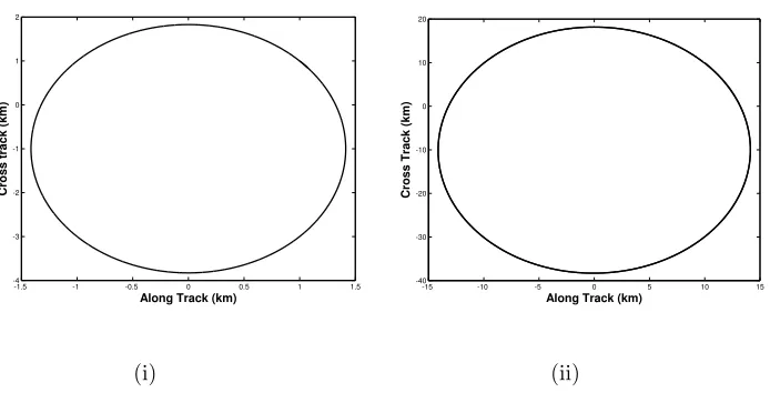
wherex0=x(0) andy0=y(0). However, using this initial condition constraint in the nonlinear model (10)

results in secular drift of the orbit which essentially means that the satellites are moving further apart with

time. This drift is illustrated in Figure 7 (i) for an initial relative distance of approximately 2kmover 100

orbits and in Figure 7 (ii) for an initial relative distance of approximately 20kmover 100 orbits.

The drift per orbit is on average 0.0211 km per orbit for the small relative distance and 0.2011 km per orbit

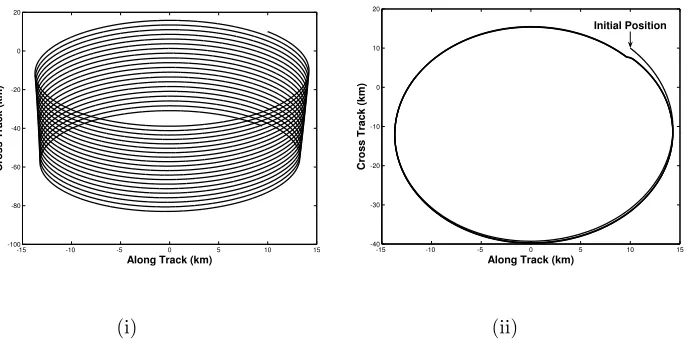
for the large relative distance. We now illustrate how TDFC can be used to counteract this undesired drift.

To implement the TDFC the second order equations (10) are converted into the form (2) by expanding the

phase space and settingu(t) =−K[ux, uy, uz]T_{. The delay time is defined in the same way as in the previous}

application by defining an appropriate Poincare section. TDFC of the form (1) is then applied to reduce the

drift between the satellites as illustrated in Figure 8 for the initially small relative distance case, with the

TDFC requirement illustrated in Figure 9 for the 20 km case.

These controls are initially large impulses, however their magnitudes reduce with time and therefore

-1.5 -1 -0.5 0 0.5 1 1.5 -4

-3 -2 -1 0 1 2

Along Track (km)

C

ro

s

s

T

ra

c

k

(

k

m

)

-15 -10 -5 0 5 10 15

-60 -50 -40 -30 -20 -10 0 10 20

Along Track (km)

C

ro

s

s

T

ra

c

k

(

k

m

)

(i) (ii)

Figure 7. Drift of Relative satellite motion: (i) the satellites are initialized close together (2 km) (ii) the

satellites are initialized far apart (20 km).

-1.5 -1 -0.5 0 0.5 1 1.5 -4

-3 -2 -1 0 1 2

Along Track (km)

C

ro

s

s

t

ra

c

k

(

k

m

)

-15 -10 -5 0 5 10 15

-40 -30 -20 -10 0 10 20

Along Track (km)

C

ro

s

s

T

ra

c

k

(

k

m

)

(i) (ii)

km) relative distance is approximately 0.1886m/sper orbit over 20 orbits reducing the drift to 2.1259×10−8

km per orbit once the control is implemented. For the initially large (20 km) relative distance the ∆V per

orbit is 13.2905m/sper orbit over 20 orbits reducing the drift to 3.8947×10−6_{km per orbit.}

0 5 10 15 20 25 30

-5 0 5 10x 10

-3

time (hours)

x

a

c

c

.

(m

/s

2)

0 5 10 15 20 25 30

-0.02 -0.01 0 0.01

time (hours)

y

a

c

c

.

(m

/s

2)

0 5 10 15 20 25 30

-10 -5 0 5x 10

-3

time (hours)

z

a

c

c

.

(m

/s

2)

Figure 9. Feedback control signal that bounds relative satellite motion where the satellites are initialized close

together (20 km)

In the following section we illustrate the effect of a perturbation by introducing the eccentricity of the

leader spacecraft.

¨

x−2ω−ω2_x+µ(r+x)

d −

µ

r2 + ˙r= 0,

¨

y+ 2ωx˙−ω2_y+µy d = 0,

¨

z+µz_d = 0,

(12)

We choose a small eccentricitye= 0.005 and simulate the equations using the initial conditions derived

in9 _{for the linearized equations of motion:}

˙

y(0)

x(0) =−

ω(2 +e)

(1 +e)1/2_(1−e)3/2 (13)

The initial condition (13) provides an initial guess for an almost periodic orbit with nonlinearities and

eccentricity perturbations. In this case the initial uncontrolled orbit (for an initial 20 km relative distance)

has a large drift of 0.2439 km and an average drift of 0.6908 km per orbit over 10 orbits, see Figure 10 (ii).

In this case the average drift increases with longer mission times. Applying TDFC to the system (12) in the

same way as for the case without the eccentricity perturbation yields the trajectory shown in Figure 10 (i)

Figure 10 (ii) illustrates the TDFC-controlled orbit. It can be seen that the initial orbit has the same drift as

before of 0.2439 km, but an average drift of 0.0145 km per orbit over 20 orbits. Therefore, in the uncontrolled

case the average drift per orbit increases with mission length whereas the average drift per orbit is decreasing

in the controlled case. The average ∆V over 20 orbits is 15.016 m/s per orbit.

In summary, this example has illustrated the effectiveness of TDFC in eliminating drift between

satel-lites. We have also demonstrated that TDFC can be useful in the presence of nonlinear and eccentricity

-15 -10 -5 0 5 10 15 -100

-80 -60 -40 -20 0 20

Along Track (km)

C

ro

s

s

T

ra

c

k

(

k

m

)

-15 -10 -5 0 5 10 15

-40 -30 -20 -10 0 10 20

Along Track (km)

C

ro

s

s

T

ra

c

k

(

k

m

)

Initial Position

(i) (ii)

Figure 10. (i) Drift of Relative satellite motion with a leader in an eccentric orbit over 10 orbits (ii)

TDFC-controlled orbit

harmonic perturbations.

It has been shown that TDFC can be used in a number of applications in astrodynamics. The examples

in this paper are simplified models and are used as motivating examples for further study. Future work

will focus on applying TDFC to more complex and realistic models. For example the application of TDFC

to bounding the satellite relative motion in low-Earth orbits would include perturbations such as zonal

harmonics and air drag. Furthermore, there are a number of extensions of TDFC that have been designed

to improve its efficiency and autonomy. Moreover, natural extensions of this work would investigate the use

of multiple delay terms (see Socolar. et .al.20_{) to improve the efficiency of the method when applied to}

these problems. In addition an investigation will be undertaken using an adaptive delay timeτ (see Yu21₎

to increase the controller autonomy.

5.

Conclusions

In this paper we have used time-delayed feedback control (TDFC) to drive trajectories of nonlinear

systems onto periodic orbits. In particular this paper has used TDFC to: (i) control the chaotic attitude

motion of an asymmetric satellite at motion in an elliptical orbit (ii) maintain a spacecraft in an orbit about

a central body with large ellipticity and (iii) bound the relative motion of two satellites flying in low Earth

orbits. Furthermore, (i) provides a motivating example of using TDFC to problems in astrodynamics through

its conventional use as a method of chaos control and applications (ii) and (iii) highlight its novel use for

bounding trajectories that are not embedded in chaotic attractors. In summary, this paper illustrates that

TDFC is an efficient tool for stabilizing and bounding spacecraft motion provided that the initial (almost

periodic) trajectory has a large instability time scale relative its orbit period. Future work will investigate

method. Furthermore, when the TDFC-controlled trajectory converges onto a periodic orbit, the Jacobian

matrix will itself be periodic. Therefore, future work will investigate analogies with Floquet theory to this

limiting case.

Acknowledgments

This work was funded by grant EP/D003822/1 from the UK Engineering and Physical Sciences Research

Council (EPSRC).

References

1

Pyragus, K., ‘Continuous control of chaos by self-controlling feedback’. Physics Letters A, Vol. 170, pp. 421-428, 1992.

2

Lewis, F. L., ‘Optimal Control’. New York: Wiley, pp. 129-214, 1986.

3

Naumenko, A. V., Loiko, N. A., Turovets, S. I. ‘Controlling extended systems with Spatially Filtered, Time-Delayed

Feedback’.Int. J. Bifurc. Chaos, Vol. 8, pp. 1791-1799, 1998.

4

Bleich, M. E., Hochheiser, D., Moloney, J. V. ‘Chaos Control in External cavity Laser Diodes using Electronic Impulsive

Delayed Feedback’.Phys. Rev. E, Vol. 55, pp. 2119-2126, 1997.

5

Brandt, M., Shih, H. T., Chen, G., ‘Linear Time-delay Feedback Control of a Pathological Rhythm in a Cardiac Conduction

Model’.Phys. Rev. E, Vol. 56, pp. 1334-1337, 1997.

6

Elmer, F. J., ‘Controlling Friction’.Phys. Rev. E, Vol. 57, pp. 4903-4906, 1998.

7

Biggs, J. D., McInnes, C. R., Waters, T., ’Control of Solar Sail Periodic orbits in the Elliptic three-body problem’, Journal

of Guidance, Control and Dynamics, Vol. 32, No. 1, pp. 318-320, 2009.

8

Biggs, J. D., McInnes, C. R., ’An optimal gains matrix for time-delayed feedback control’, 2nd IFAC conference on the

Control of Chaos, London, June 2009.

9

Inalhan, G., Tillerson, M., How, J. P., ‘Relative Dynamics and Control of Spacecraft Formations in Eccentric Orbits’.

Journal of Guidance, Control and Dynamics, Vol. 25, No. 1, pp. 48-59, 2002.

10

Chen, L.Q., Liu, Y.Z., ‘Chaotic attitude motion of a class of spacecraft in an elliptic orbit.’ Technishe Mechanik 18 1 pp.

4144, 1998.

11

Nakajima, H.,‘On analytical properties of delayed feedback control of chaos’. Physics Letters A, Vol. 232, pp. 207-210,

1997.

12

Nakajima, H., Ueda, Y., ‘Limitation of generalized delayed feedback control’. Physica D, 111, pp. 143-150, 1998.

13

Fiedler, B., Flunkert, V., Georgi, M., Hovel, P. Scholl, E., ‘Refuting the Odd-Number Limitation of Time delayed Feedback

Control’.Physical Review Letters, Vol. 98, pp.1-4, 2007.

14

Just, W., Fiedler, B., Georgi, M., Flunkert, V., Hovel, P., and Scholl, E., ‘Beyond the odd number limitation: a bifurcation

analysis of time-delayed feedback control’. pp.Physical Review E, Vol. 76, 026210, 2007.

15

Postlethwaite, C. M., Silber, M., ‘Stabilizing unstable periodic orbits in the Lorenz equations using time-delayed feedback

control’.Physical Review E, Vol. 76, 056214, 2007.

16

Scheeres, D. J., ‘The effect ofC22on orbit energy and angular momentum.’ Celestial Mechanics and Dynamical Astronomy,

73, pp. 339-348, 1999.

17

Scheeres, D. J., Williams, B. G., Miller, J. K. ‘Evaluation of the Dynamic Environment of an Asteroid: Applications to

18

Koon, W-S., Marsden, J., Ross, S., Lo. M., and Scheeres, D., ‘Geometric Mechanics and the Dynamics of Asteroid Pairs’.

Annals of the New York Academy of Science, 1017, pp. 11-38, 2004.

19

Clohessy, W. H., Wiltshire, R. H., ‘Terminal Guidance System for Satellite Rendezvous’. Journal of the Aerospace

Sciences, vol. 27, pp.653-658, 1960.

20

Socolar, J.E.S., Sukow, D.W., and D.J. Gauthier, D.J., ‘Stabilizing Unstable Periodic Orbits in Fast Dynamical Systems’,

Phys. Rev. E, vol. 50, pp. 3245-3248, 1994.

21_{Yu, X.,‘Tracking Inherent Periodic Orbits in Chaotic Dynamic Systems via Adaptive Variable Structure Time-Delayed}

Self Control’. IEEE Trans. on Circuits and systems-I: Fundamental Theory and applications, Vol. 46, No.11, pp. 1408-1411,

November 1999.

6.

Appendix

In this Appendix we derive the necessary conditions for TDFC to optimality drive a trajectoryX(t) onto

a periodic orbit and use these conditions to construct a suitable gain matrixK.

As X(t) is a solution of the original system (2) with u(t) = 0 then the delayed trajectory is also a

solution, namely:

˙

X(t−τ) =f(X(t−τ)), (14)

subtracting (14) from (2) yields the error dynamical system:

˙

e(t) =F(e(t)) +Bu(t), (15)

where e(t) = X(t)−X(t−τ) and F(e(t)) = f(X(t))−f(X(t−τ)). Additionally, taking the Taylor

expansion off(X(t)) about the delayed trajectoryX(t−τ) gives:

f(X(t)) =f(X(t−τ)) +A(t)(X(t)−X(t−τ)) + [H.O.T], (16)

whereA(t) = ∂f(X(t))

∂X(t)

¯ ¯ ¯_X

(t−τ)and [H.O.T] are higher order terms. It follows that:

F(e(t)) =A(t)e(t) + [H.O.T]. (17)

Assuming that the initial errore(t) is small enough, we may neglect higher order terms ine(t) and therefore

(15) and (17) yield the linear time-varying system:

˙

e(t)=A(t)e(t) +Bu(t). (18)

For the controlled system (18), we wish to minimize a function of e(t) and the total control effort. This

is clearly a desirable cost function for spacecraft applications as it would minimize fuel expenditure and

prolong mission life while maintaining accurate tracking. Such a performance index for this objective can

be expressed as:

1 2

∞ Z

0

¡

eT(t)Qe(t) +uT(t)Ru(t)¢

whereQandRare real symmetric positive definite matrices. Therefore, it follows from the theory of optimal

control for linear time-varying systems2_{that the optimal tracking control is the time-delayed feedback control}

u(t) =−Ke(t) =−K(X(t)−X(t−τ)) withK=R−1_BT_{P(t) whereP(t) is a solution of the equation:}

˙

P(t) =P(t)BR−1BTP(t)−A(t)TP(t)−P(t)A(t)−Q. (20)

whereP(t) is assumed to be a continuous function with continuous first order derivatives for existence and

uniqueness of the solution. We note that this construction is convenient for some practical situations, since

it does not require any reference orbit, that is, the computation of the gain matrix is about the delayed

trajectory.

In order to use the Riccati equations (20) to construct a practical gain matrix we first have to tune the

matricesQ andR. This is conveniently achieved by settingQ=Idn×n where Idn×n is then×n identity

matrix wheren is the dimension ofX(t). Then we defineR=βIdm×n wheremis the number of controls

and β is a free parameter. This reduces the tuning problem to finding an appropriate value of β which

weights the control cost relative to the periodicity cost. Moreover, if β is weighted in favor of minimizing

control effort this may result in poor tracking of the delay trajectory and thus it will become less periodic.

Conversely if β is weighted in favor of minimizing periodicity by a significant amount this may result in a

much larger ∆V requirement and fuel expenditure.

The initial conditionP(0) can be evaluated using the Riccati algebraic equation (i.e. with ˙P(0) = 0) with

A(0) evaluated at the initial point of the trajectory. Following this we numerically integrate the equations

(20) simultaneously with the equations of motion with the initial conditions ˙P(0) = 0, P(0), A(0), B, Q, R

to yield P(t). Note that the Riccati equations and the nonlinear equations of motion are coupled, so the

computational effort is far greater when compared to using a constant gain matrix. If it is essential to keep

computations to a minimum, periodic and constant gain matrix approximations may be used. Moreover, as

TDFC drives the trajectory onto a periodic orbit, the matrixP(t) will be asymptotically periodic. Therefore,

an approximate periodic gain matrix can be derived using this asymptotically periodic solution to the Riccati

equations. Furthermore, if the amplitude of oscillation of the asymptotically periodic components ofP(t) are

small relative to their averaged values, the averaged values can be used to derive an approximately optimal