Multi-disciplinary robust design of variable speed wind turbines

MULTI-DISCIPLINARY ROBUST DESIGN OF VARIABLE

SPEED WIND TURBINES

Edmondo Minisci?, Sergio Campobasso

School of Engineering University of Glasgow

James Watt S.B., G12 8QQ, Glasgow, UK Email: {edmondo.minisci,sergio.campobasso}

@glasgow.ac.uk

Michele Dellantonio Dipartimento di Ing. Elettrica Universit`a di Padova

via Gradenigo 6/A, 35131, Padova, Italy Email: [email protected]

Andrea Montecucco School of Engineering University of Glasgow

Rankine Building, G12 8LT, Glasgow, UK Email: [email protected]

Massimiliano Vasile

Department of Mechanical & Aerospace Engineering, University of Strathclyde 75 Montrose Street, G1 1XJ, Glasgow, UK Email: [email protected]

Abstract. This paper addresses the preliminary robust multi-disciplinary design of small wind turbines. The turbine to be designed is assumed to be connected to the grid by means of power electronic converters. The main input parameter is the yearly wind distribution at the selected site, and it is represented by means of a Weibull distribution. The objective function is the electrical energy delivered yearly to the grid. Aerodynamic and electrical characteristics are fully coupled and modelled by means of low- and medium-fidelity models. Uncertainty affecting the blade geometry is considered, and a multi-objective hybrid evolutionary algorithm code is used to maximise the mean value of the yearly energy production and minimise its variance.

Key words: Multi-Disciplinary Optimisation, Robust Design, Integrated System Design, Evolutionary Computation, Wind Energy, Aerodynamic and Electrical Op-timisation.

1 Introduction

financial and logistic requirements of suitable experimental campaigns, and also to last-minute design alterations aimed at improving component matching.

On the other hand, the use of a simulation-based fully coupled approach since early stages of the design would allow the wind energy industry to both reduce development costs and time-scales, and develop more efficient turbines. The benefits and the effectiveness of adopting the fully coupled design strategy since early stages of the product design have been known and exploited for a long time in other engineering fields such as aircraft3 _{and turbomachinery}4 _{design. To the best of}

the author’s knowledge, however, the development and the application of the fully coupled strategy for wind turbine conceptual and preliminary design have not been suitably explored yet.

The fully coupled design optimisation approach is computationally more demand-ing than the faster conventional uncoupled design strategy. However, the high per-formance of modern computers and the increasing availability of parallel computing resources allow numerical optimisation to handle complex multidisciplinary design problems in relatively short rimes. These circumstances presently enable one to model all the sub-systems using diverse fidelity levels and directly proceed with the integrated design of the whole system.

This paper presents an integrated approach to the preliminary multi-disciplinary robust design of small variable speed horizontal axis wind turbines. The attribute ’robust’ stems from the fact that the effects of uncertainty such as that due to manufacturing and assembly tolerances on the objective functions and constraints is carefully taken into account in the design optimisation5_{. The turbines of the}

considered class have rated power of up to about 50 kW and feature a permanent magnet generator and an inverter. The multidisciplinary analysis system consid-ered herein couples the aerodynamic and electrical characteristics of the turbine, and models them by means of low- and medium-fidelity models. The main input parameters are the yearly wind distribution at the selected site and the rotor swept area. The objective of the design optimisation is to maximise the yearly energy harvest. This quantity corresponds to the energy delivered to the grid, since it is assumed that the turbine system is directly connected to the grid. Given that the optimisation is carried out taking into account uncertainty of the design variables, the robust optimisation actually consists of maximising the mean of the yearly en-ergy production and minimising its standard deviation. As shown in the remainder of this paper, this optimisation specifications result in the occurrence of a Pareto front.

The uncertainty affecting the design variables can be due to several stochastic factors, including manufacturing and assembly tolerances and wear. In the present study, the Univariate Reduced Quadrature (URQ) approach to uncertainty propaga-tion in robust design optimisapropaga-tion is used6_{. The estimate of mean and variance of the}

stochasticastic variable, characterised by a mean and a standard deviation. In the robust optimisation process, the output of each robust analysis is used by a multi-objective evolutionary algorithm (EA), whose multi-objectives are the maximisation of the mean value of yearly energy production and the minimisation of its variance.

The adopted EA hybridises the Multi-Objective Parzen based Estimation of Dis-tribution (MOPED) algorithm7,8_{, and the Inflationary Differential Evolution}

Algo-rithm (IDEA)9_{, where MOPED is used to explore the search space and converge}

to a preliminary approximation of the Pareto front, while IDEA is then adopted to further push some of the best solutions towards the true Pareto front.

The aerodynamic and electrical models are described in section 2, whereas the main features of the two adopted optimisers and their use in this work are reported in section 3. The set-up and the results of a wind turbine robust design optimisation are provided in section 4. Then, a conclusion section summarises the work and anticipate future developments.

2 System Models

The wind energy conversion system (WECS) considered in this paper can be divided into two main parts: an aerodynamic part and an electro-mechanical part. The former consists of the bladed rotor, while the latter is made up of a permanent magnet synchronous generator and power electronic converters.

2.1 Aerodynamic model

The aerodynamic module of the integrated analysis system is a blade-element momentum (BEM) theory code10, developed at the School of Engineering of Glasgow University. This low-fidelity analysis tool is based on the radial subdivision of the bladed rotor into sections or strips. The BEM model used in this work includes the wake rotation. For each strip, the flow data and the aerodynamic forces are determined by equating the thrust and the torque computed with the classical lift and drag theory on one hand, and the conservation of the one-dimensional linear and angular momentum on the other. Tip and hub vortex losses are also included by means of the Prandtl tip loss model. The aerofoil lift and drag coefficient data are stored in tables as functions of the Reynolds number and the relative angle of attack, and such data are computed in a pre-processing step using the MIT aerodynamic solver XFOIL.

The set of input variables of the BEM code is made up of: freestream wind velocity, angular speed of the rotor, number of blades and blade geometry. This latter is defined by root and tip radius, and radial distributions of chord and twist angle. The set of output variables includes: aerodynamic power, axial thrust on the rotor, bending moment at the blade root and radial distributions of all flow data (e.g. axial and circumferential induction factors) and aerodynamic forces. As pointed out in the remainder of the paper, a single and constant aerofoil geometry is used throughout the design optimisation, and for this reason the lift and drag coefficient tables can be computed in a preprocessing step.

2.2 Electrical Model

can be fed into the grid. For small wind turbines, permanent-magnet synchronous generators (PMSGs) offer significant benefits over induction generators: higher per-formance, gearbox-less operation, lower weight and smaller size11. Therefore the main component of the electrical model is a PMSG to convert mechanical energy into electrical energy. The choice of the power electronics for interfacing such a generator to the grid is based both on the control requirements of an actual system and on the speed and easiness of the simulation.

A diode bridge rectifier is chosen for the greater simplicity of its control with respect to that of a controlled AC/DC converter. A grid-side inverter controls the reactive and active power supplied to the grid12_{. The incorporation of a DC/DC converter}

in between the rectifier and the inverter enables one to achieve the following bene-fits14,13,15:

1. Tight control of the generator-side voltage to achieve rotor speed control

2. Increase of voltage operating range while maintaining appropriate inverter-side DC voltage

3. Ease and flexibility of the inverter control

4. Reduced losses with Selective Harmonic Elimination (SHE)

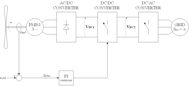
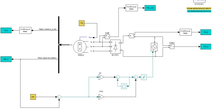
A boost chopper is chosen as DC/DC convert and the described configuration is showed in Figure 1. It is assumed that there is infinite short-circuit power at the connection node, i.e. the voltage at this node is considered constant, and the iron core saturation and losses of the PMSG are neglected, as they are usually much smaller than the other losses. The model is implemented in Simulink using the Sim-PowerSystems toolbox (Figure 2 shows the Simulink model).

The inverter control can be designed to keep the DC-link voltage VDC2 constant

Figure 1: Diagram of the whole electro-mechanical system

varying the reactive power to maximise the real power supplied to the grid16_.

There-fore the output voltage of the boost converter is constant so that regulating its duty cycle (d) it is possible to control the rectifier output VDC1 using the relationship

d= VDC2−VDC1 VDC2

Thus the voltage at the PMSG’s terminals, which influences the rotor speed, can be controlled by a Maximum Power Point Tracking (MPPT) algorithm, which decides what operating mechanical speed to use in order to maximise the overall power produced by the system. The MPPT control is performed by the actual operat-ing WECS, and not duroperat-ing simulation. For this reason and in order to make the simulation faster, the electrical system downstream of the diode rectifier has been modelled as an ideal DC voltage source, whose voltage is controlled depending on the desired mechanical speed requested by the optimiser.

The input variables of the electrical model are the mechanical speed ωm,ref (rad/s) and the torque Tm (Nm), which come from the BEM code. A PI controller is used to impose the mechanical speed while the torque is directly set in the PMSG block. The PI controller regulates VDC1 in order to set the desired speed. The considered

parameters for the PMSG are the number of poles p, the flux induced in the stator windings by the magnets φ (Wb), the nominal voltage Vn (V) and the maximum electrical frequencyfe,max. The parasitic effects of the components are constant and estimated from commercially-available components.

Figure 2: Simulink model

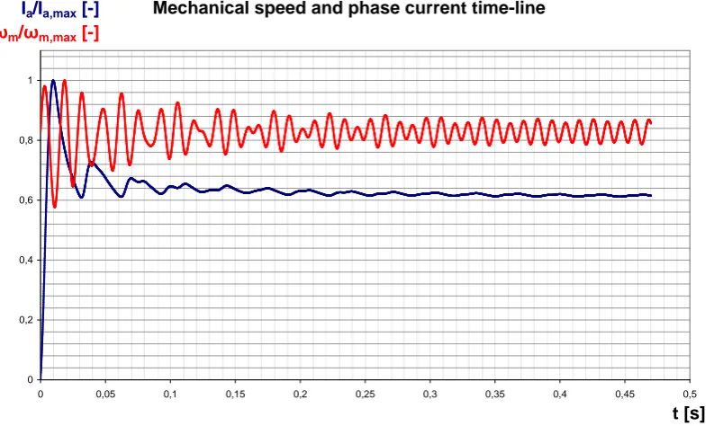
Before reaching steady-state, the simulation encounter a transient, whose time is function of the electrical (resistances, capacitances and inductances) and mechanical (torque and inertia) parameters (Figure 3). The output variables of the Simulink model are the mechanical speedω∗_m(t), the DC bus voltageVdc1(t), the PMSG phase

current Ia,RM S, the PMSG phase-to-phase voltageVab,RM S, and the DC bus current

IDC. After the simulation, losses are classified and computed as follows:

• mechanical losses due to viscous friction:

Pl,m =b ω∗2m

Mechanical speed and phase current time-line

0 0,2 0,4 0,6 0,8 1

0 0,05 0,1 0,15 0,2 0,25 0,3 0,35 0,4 0,45 0,5

t [s]

Ia/Ia,max [-]

ω_m/ω_m,max [-]

Figure 3: Mechanical speed and phase current time-line (model input: ωm= 7rad_s , Tm= 3300N m)

• losses of the PMSG and rectifier:

Pl,AC = [3(Rs+Rline) + 2Rbr)]Ia,RM S2

whereRsandRlineare the PMSG winding resistances andRbr is the resistance modeling the conduction losses on the diode bridge rectifier;

• losses on the DC/DC converter:

Pl,L =RDCIDC2

Pl,s =Rsw(IDC √

D)2 Pl,d =Rd(IDC

√

1−D)2

where RDC is the inductor resistance, Rsw is the switch on-resistance and Rd is the diode conduction resistance;//

• losses on the inverter:

Pl,inv = (1−ηinv)(VDC1IDC−Pl,L−Pl,s−Pl,d)

where ηinv is the inverter efficiency, which is assumed to be constant in the project operative range.

Once the losses have been determined, the electric model computes several interme-diate efficiencies and the total one as:

• PMSG and rectifier efficiency:

ηAC =

VDC1IDC

• DC/DC converter efficiency:

ηDC =

1 1+ Vd

VDC2+

[RDC+DRsw+(1−DRd)]IDC VDC2

where Vd is the forward voltage of the diode;

• total efficiency:

ηtot = 1− P

Pp

Pm

The outputs of the model are the total efficiency of the electrical system ηtot and the power supplied to the grid Pgrid.

2.2.1 Model validity boundaries

In order to have feasible solutions, the PMSG nominal voltage Vn and the maxi-mum electrical frequency fe,max must be bounded by the actual limits of a physical system. FromVnand fe,max depend other design parameters, such as the number of pole pairs p and the flux φ. The nominal voltage is the maximum voltage that the synchronous machine can generate. This parameter affects the winding insulation required and the output current; with a higher voltage, the current and thus the losses are lower, but a high voltage requires a great number of poles and a high flux. In a real PMSG the maximum frequency is imposed by the iron losses, and by the skin effect in the winding conductors. The former is the sum of hysteresis and eddy currents losses,Pl,iron =khyfBˆ2+kecf2Bˆ2, while the latter is characterised by the depth of penetration δ=q ρ

πfeµ0. If the frequency is high, then δ is small and the

current flows in the conductor surface, increasing the Joule losses. Therefore a limit on the frequency value is necessary to avoid that a possible optimum configuration demands a high value offe. A minimum frequencyfe,minis required too, because the generator cannot work with small frequencies. For these reasonsVn is the maximum voltage at the PMSG’s terminals and fe,min ≤fe ≤fe,max.

Therefore the following boundaries must be considered:

• mechanical speed range: ωm,min ≤ω≤ωm,max;

• mechanical power range: Pm,min ≤Pm ≤Pm,max;

• mechanical torque: Tm,min ≤Tm ≤Tm,max

where

Tm,min=

Pm,min

ωm,max

Tm,max=

Pm,max

ωm,min

(2)

These relationships allow to estimate the range of the parameters p ∈ [pmin, pmax] and φ ∈[φmin, φmax] as

pmin =

2πfe,min

ωm,max

pmax =

2πfe,max

ωm,min

(3)

φmin =

Vn √

3ωm,maxpmax

φmax =

Vn √

3ωm,minpmin

where the RMS value of the fundamental EMF induced in the stator windings is E = √Vn

3 =p φ ωm.

The parameters Vn and [fe,min, fe,max] are imposed as boundaries, while pand φ are considered values to optimize. For each values of torque and mechanical speed, the program starts the simulation searching for the values ofpand φ that maximise the electrical energy produced in one year.

First, the MATLAB script calculates the PMSG’s voltageV and electrical frequency fe and checks that they are not outside the imposed boundaries, using the relation-ships

fe,min≤

fe=

pωm 2π

≤fe,max (5)

V =√3p φ ωm ≤Vn (6)

If the boundaries are satisfied, the simulation starts, otherwise the program returns a value of injected power to the grid Pgrid calculated as

Pgrid =

Pm

10_f|∆f|

e,max

|∆V|

Vn

(7)

where ∆f and ∆V are the difference between the imposed limit (of frequency and/or voltage) and the calculated values using Eq. 5 and 6.

It is not possible to reach steady-state with high values of mechanical torque Tm and/or low values of mechanical speed ωm, φ or p. In these cases the mechanical speed does not converge to the set value ωm,ref because the PMSG cannot generate the requested voltage to ”brake” the rotor at the requested low speed and high torque. Vice versa, when the required speed is too high for the set torque value it is possible to reach steady-state, but with a lower mechanical speed than the reference ωm,ref. The mean value of the effective mechanical speed ωm∗ is computed and compared to the reference speed ωm. If the difference satisfies the equation ∆$=|ω_m∗ −ωm| ≤ ω₅m then the program computes the losses and the power Pgrid,

otherwise the program sets Pgrid =

Tmω∗m

|4$|. These two conditions are important for the correct functioning of the optimizer when it falls into those particular cases.

3 Evolutionary Hybrid solver

As previously stated, the adopted solver is an hybrid code which uses MOPED and IDEA, both previously developed by some of the authors in the framework of aerospace design and optimisation field.

The MOPED (Multi–Objective Parzen based Estimation of Distribution) algo-rithm is a multi–objective optimisation algoalgo-rithm for continuous problems that uses the Parzen method to build a probabilistic representation of Pareto solutions, with multivariate dependencies among variables7,8_{. Some techniques of NSGA-II}17 _are

used to classify promising solutions in the objective space, while new individuals are obtained by sampling from the Parzen model. NSGA-II was identified as a promis-ing base for the algorithm mainly because of its intuitive simplicity coupled with excellent results on many problems.

Probability Density Function (PDF) in the mean square sense. Should the true PDF be uniformly continuous, the Parzen estimator can also be made uniformly consistent. In short, the method allocates Nind identical kernels (where Nind is the number of individuals of the population of candidate solutions), each one centred on a different element of the sample.

By means of the Parzen method, a probabilistic model of the promising search space portion is thus built on the basis of the information given byNindindividuals of the current population, and τENind new individuals (τE ≥ 1) can then be sampled . The variance associated to each kernel depends on (i) the distribution of the individuals in the search space and (ii) the fitness value associated to the pertinent individual, so as to favour sampling in the neighbourhood of the most promising solutions. In order to improve the exploration of the search space it is sometimes useful to alternatively adopt two different kernels when passing from one generation to the following one.

The nature itself of the algorithm often prevents the precise reaching of the Pareto front. Especially when the front is broad and individuals of the population are spread over different and far areas in the domain space. From here the idea to couple MOPED with another advanced evolutionary algorithm, which has better convergence properties.

For design and optimisation in other engineering areas, some of the authors devel-oped an improved version of differential evolution (DE). The new algorithm, IDEA, is based on a synergic hybridisation of a differential evolution variant and the logic behind monotonic basin hopping (MBH)18_{. The resulting algorithm demonstrated}

to outperform DE and MBH on some difficult space trajectory design problems, whose search space has a (multi) funnel like structure. In this work a modified version of IDEA will be used to push individuals lying on the approximated Pareto front resulting from MOPED process, further toward the true front.

The main algorithm of IDEA is detailed in litterature9, while here we will just recall the practical aspects of the algorithm. Basically, a DE process is performed several times and each process is stopped only when the population contracts under a predefined threshold. Every time that the DE stops, a local search is performed in order to properly converge to the local optimum. Since for non–trivial functions it is extremely easy to converge to only local optima, the DE+local search is iterated several times, considering either local restart or a global one, on the basis of a predefined scheduling.

For this work, since the optimisation is constrained, the internal DE mechanism must be modified and the comparison of individuals during the DE process must take into account constraints as well. Constraint handling technique in this case is borrowed from what usually done in evolutionary computation and also in MOPED. Basically, when parents and offsprings are compared, offsprings are chosen if they have a better constraint compatibility, cp, and in case cp of offspring and parent is the same (when the constraints are satisfied both for the parent and the children), then the objective function is considered.

When MOPED reaches the maximum number of generations, clustered sup-populations form the current front are given to IDEA as initial solutions. Since IDEA is still single objective, individuals picked up from final MOPED population are pushed forward considering a weighted sum of the original objective functions.

current problem is totally unknown, and could be multi-funnel like and extremely noisy. Noise is expected to be introduced by both the aerodynamic and the electric solvers. The adopted code, by mixing the exploratory capabilities of MOPED and the convergence characteristics of IDEA, should guarantee a satisfying robustness.

4 Optimisation setting and results

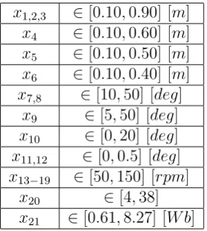
The turbine blade shape is parametrised by means of 6 design parameters defining the radial chord distribution, and 6 design parameters defining the radial twist distribution. Additional parameters define the rotational speed for each considered wind speed, as well as poles and flux for the design of the generator. Since in this case we considered 7 wind speeds from 6m/s to 12m/s, the total number of design parameters is 21. Bounds for design parameters are given in Table 1. Internal and external blade radius are not allowed to change and fixed to 1.3[m] and 6.3[m], respectively.

x1,2,3 ∈[0.10,0.90] [m]

x4 ∈[0.10,0.60] [m]

x5 ∈[0.10,0.50] [m]

x6 ∈[0.10,0.40] [m]

x7,8 ∈[10,50] [deg]

x9 ∈[5,50] [deg]

x10 ∈[0,20] [deg]

x11,12 ∈[0,0.5] [deg]

x13−19 ∈[50,150] [rpm]

x20 ∈[4,38]

x21 ∈[0.61,8.27] [W b]

Table 1: Bounds of design parameters

Parameters to be set for the MOPED algorithm are size of the population, Nind, number of constraint classes,Ncl, the fitness parameter,αf, the sampling proportion,

τE, and, in this case, they were set as: Nind = 100, NgenM AX = 100, Ncl = 3;

αf = 0.5;τE = 1.

Since the adopted algorithms are built to minimise objective functions, the prob-lem is set in order to have two objectives to minimise:

F1 = 1e6−ET E

F2 =σ2T E

(8)

where ET E and σ2T E are the mean value of the annual energy production ([kWh]) and its variance, respectively.

While, considered constraints are:

C1 :F1 ≤9.6e5

C2 :F2 ≤2e7

C3 :EMB ≤12

(9)

where MB is the bending moment ([kNm]) at the blade root and EMB is its mean

In order to compute statistical values to be used as objective and constraint functions, parameters defining the blade geometry are supposed to be uncertain parameters with gaussian distributions, centred on nominal values of parameters and have a standard deviation σ = 0.03 (it must be noted that all the solvers work on a non-dimensional search space, where all variables vary ∈ [0,1]). Since only the 12 parameters defining the shape of the turbine blade are considered affected by uncertainty, and the deterministic sampling method requires 2n+ 1 evaluations, then, for this test case, each solution evaluation actually requires 25 computations of the full annual energy production6.

Parameters of DE in IDEA are set as: weighting factor, F = 0.9, crossover probability,CR= 0.9, strategy “DE/best/1/bin”. IDEA stops when the population contracts to 25% of maximum expansion during the evolution.

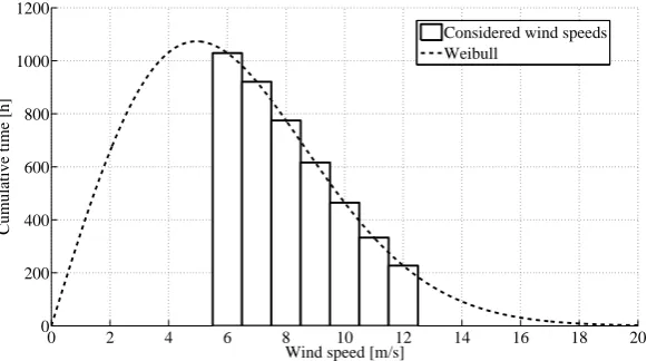
Considered speeds and relative cumulative timing to compute the annual energy production are shown in Figure 4, and are derived considering a weibull distribution with scale parameter λ= 7 and shape parameter k = 2.

0 2 4 6 8 10 12 14 16 18 20

0 200 400 600 800 1000 1200

Wind speed [m/s]

Cumulative time [h]

Considered wind speeds Weibull

Figure 4: Wind speeds and cumulative timing considered to compute the annual energy production

4.1 Optimisation results

The whole code is implemented in MATLABR and parallelised on a linux cluster, in order to speed-up the optimisation process.

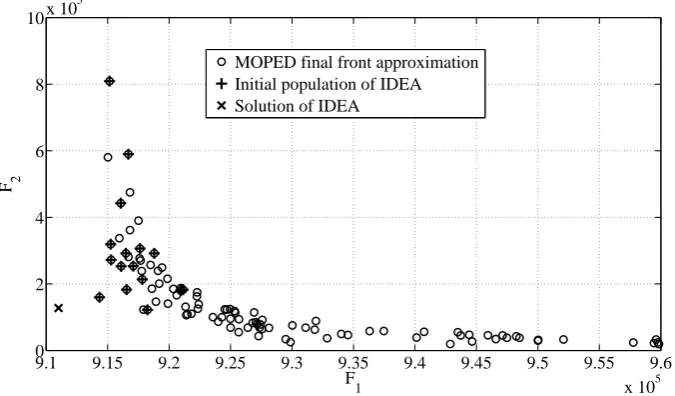
After 10k function evaluations MOPED is able to approximate the Pareto front as shown in Figure 5. Pareto solutions were clustered in the search space and the sub-population containing the solution minimising F1 was considered as the

9.1 9.15 9.2 9.25 9.3 9.35 9.4 9.45 9.5 9.55 9.6 x 105 0

2 4 6 8 10x 10

5

F

1

F 2

MOPED final front approximation Initial population of IDEA Solution of IDEA

Figure 5: Solution of the optimisation process: Pareto front approximation found by MOPED, and final solution of the whole process after IDEA refinement.

At this point it is worth considering the cost of the refinement. If we take into account that the dimension of DE population was 17, the DE refinement required near 2400 evaluations, and that each function evaluation of fmincon includes the approximation of the local gradient, then the refinement of just one solution costed near 11k function evaluations, most of which required by fmincon to improve the solution of just 60 kWh. The deterministic sampling6 allows to efficiently compute the gradients of statistical values, but in this case we used fmincon to approximate them. Future tests will allow to compare performance when gradients are computed directly by the deterministic sampling and by fmincon.

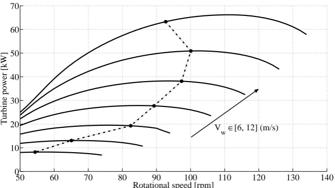
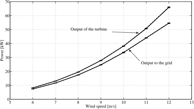
The geometry of the optimal blade is shown in Fig. 6, while Figures 7 and 8 show the power curve of the turbine and the one referred to the entire chain up to the grid, respectively. Note that here the nominal results referred to the nominal blade are shown, which are not the statistical values considered by the searching codes.

It appears that the obtained solution should at rotational speeds maximising the power to the grid for each velocity, with some exceptions. In particular, operational point for Vw = 10m/s is extremely close to the validity limit of the electric model, and that can disturb the computation of statistical values, preventing the nominal blade working at maximum power. Moreover, the machine cannot work at maximum power forVw = 12m/sdue to the constraint on the maximum root bending moment, and a working point different from the maximum one must be adopted.

Final optimal point has the second objective function of just 127500kW h2_,

mean-ing a standard deviation as small as 357kW h. This result was obtained further refining a solution sampled from the MOPED final population, without considering the variance of the energy.

1 2 3 4 5 6 7 0

0.5 1 1.5 2

Radius [m]

Chord [m]; Twist/10 [deg]

Twist Chord

Figure 6: Nominal shape of the blade maximising the annual energy production as resulting from single objective refinement by IDEA

50 60 70 80 90 100 110 120 130 140 0

10 20 30 40 50 60 70

Rotational speed [rpm]

Turbine power [kW]

V_w∈[6, 12] (m/s)

Figure 7: Turbine power curves of the nominal optimal blade

5 Conclusions

A hybrid evolutionary algorithm has been applied to the integrated robust design of a wind turbine system to maximise the annual energy production. Aerodynamic and electric components have been modelled and coupled to predict the energy that can be feeded to the grid.

The work demonstrates that such integrated approach is now possible, due to advances in evolutionary techniques and, overall, increased performance of modern computational systems, and it can be fruitfully used as main tool for preliminary design of wind systems. Nonetheless, the whole robust design approach remains computationally demanding and does not allow to run the code several times, as it should be done when dealing with stochastic solvers.

50 60 70 80 90 100 110 0

10 20 30 40 50 60

Rotational speed [rpm]

Power to grid [kW]

V_w∈[6, 12] (m/s)

Figure 8: Power curves of the total system, considering the turbine and the electric chain up to the grid

5 6 7 8 9 10 11 12 13

0 10 20 30 40 50 60 70

Wind speed [m/s]

Power [kW]

Output of the turbine

Output to the grid

Figure 9: Power curve of the total system: maximum power as function of the wind speed

work will be focused on inserting into the process a multi-fidelity method as well as meta-modelling techniques. Moreover, in order to obtain realistic blade shapes with lower computational costs, the parametrisation of the blade should also consider manufacturing criteria and costs.

REFERENCES

[1] A. Rolan, A. Luna, G. Vazquez, D. Aguilar and G. Azevedo, Modeling of a Variable Speed Wind Turbine with a Permanent Magnet Synchronous Gen-erator, IEEE International Symposium on Industrial Electronics (ISlE 2009), Seoul Olympic Parktel, Seoul, Korea July 5-8 (2009).

[3] I. Kroo, S. Altus, R. Braun, P. Gage and I. Sobieski, Multidis-ciplinary Optimization Methods for Aircraft Preliminary Design, Fifth AIAA/USAF/NASA/ISSMO Symposium on Multidisciplinary Analysis and Optimization Panama City, AIAA 94-4325, Florida, September 7-9 (1994).

[4] Y. Panchenko, H. Moustapha, S. Mah, K. Patel, M.J. Dowan and D. Hall, Preliminary Multi-Disciplinary Optimisation of Turbomachinery Design, RTO AVT Symposium on ’Reduction of Military Vehicle Acquisition Time and Cost through Advanced Modelling and Virtual Simulation’, RTO-MP-089, Paris, France, 22-25 April (2002).

[5] G.J. Park, T.H. Lee, K.H. Lee and K.H. Hwang, Robust Design: An Overview, AIAA Journal, 44(1), 181-191, (2004).

[6] M. Padulo, M.S. Campobasso and M.D. Guenov, A Novel Uncertainty Propaga-tion Method for Robust Aerodynamic Design, AIAA Journal, 49(3), 530-543, (2011).

[7] M. Costa and E. Minisci, MOPED: a multi-objective Parzen-based estimation of distribution algorithm,In Proc. of EMO 2003,Faro, Portugal, 282-294, (2003).

[8] G. Avanzini, D. Biamonti, and E.A. Minisci, Minimum-fuel/minimum-time ma-neuvers of formation flying satellites,Adv. Astronaut. Sci.,116(III), 2403–2422, (2003).

[9] M. Vasile, E. Minisci and M. Locatelli, An Inflationary Differential Evolu-tion Algorithm for Space Trajectory OptimizaEvolu-tion, Evolutionary Computation, IEEE Transactions on, 15(2), 267-281, (2011).

[10] J. Manwell, J. McGowan, and A. Rogers, Wind Energy Explained. Theory, Design and Application, John Wiley and Sons Ltd., (2002).

[11] M. Heydari, A. Yazdian Varjani, M. Mohamadian, and H. Zahedi, A Novel Variable-Speed Wind Energy System Using Permanent-Magnet Synchronous Generator and Nine-Switch AC/AC Converter. 2nd Power Electronics, Drive Systems and Technologies Conference, 2011, 5–9, (2011).

[12] S.H. Song, S.I. Kang, and N.K. Hahm, Implementation and control of grid con-nected AC-DC-AC power converter for variable speed wind energy conversion system. Eighteenth Annual IEEE Applied Power Electronics Conference and Exposition, 2003. APEC ’03., 00(C), 154–158, (2003).

[13] J.A. Baroudi, V. Dinavahi, and A.M. Knight. A review of power converter topologies for wind generators. IEEE International Conference on Electric Machines and Drives, 2005, 458–465, (2005).

[14] Z. Chen and E. Spooner. Grid power quality with variable speed wind turbines. IEEE Transactions on Energy Conversion,16(2), 148–154, (2001).

[16] Z. Chen and E. Spooner. Grid interface options for variable-speed, permanent-magnet generators. IEE Proceedings - Electric Power Applications, 145(4), (1998).

[17] K. Deb, A. Pratap, S. Agarwal, and T. Meyarivan. A Fast and Elitist Mul-tiobjective Genetic Algorithm: NSGA-II. IEEE Transaction on Evolutionary Computation, 6(2), 182–197, april 2002.