Hyperspectral sub-pixel target detection using hybrid algorithms and Physics Based Modeling

Theses

Thesis/Dissertation Collections

11-18-2005

Hyperspectral sub-pixel target detection using

hybrid algorithms and Physics Based Modeling

Emmett J. Ientilucci

Follow this and additional works at:

http://scholarworks.rit.edu/theses

This Dissertation is brought to you for free and open access by the Thesis/Dissertation Collections at RIT Scholar Works. It has been accepted for

inclusion in Theses by an authorized administrator of RIT Scholar Works. For more information, please contact

[email protected].

Recommended Citation

by

Emmett

J.

Ientilucci

A.A.S.Monroe Community College, 1986

B.S

.

Rochester Institute of Technology

,

1996

M.S. Rochester Institute of Technology

,

1999

A dissertation

submitted

in partial fulfillment

of

the

requirements for the degr

ee

of Doctor

of

Philosophy

in the Chester F. Carlson Center for Imaging Science

Rochester Institute

of

Technology

November 18, 2005

Emmett lentilucci

Signature of the Author

_ _ _ _ _ _ _

. _ _ _ _ _ _ _ _ _ _ _ _

_

Accepted by

Name Illegible

/(

ROCHESTER, NEW YORK

CERTIFICATE OF APPROVAL

Ph.D.

DEGREE DISSERTATION

The Ph.D. Degree Dissertation of Emmett J. Ientilucci

has been examined and

approved

by the

dissertation

committee

as

satisfactory for the

dissertation required for the

Ph.D. degree

in Imaging Science

John R. Schott

Dr. John R. Schott

, Dissertation Advisor

Harvey E. Rhody

Dr. Harvey E. Rhody

John P. Kerekes

Dr. John P. Kerekes

P. 8ajorski

Dr. Peter Bajorski

/1

/;

1

/2c;J~)

7--Date

7

/

Title of

Dissert

ation:

Hyperspectral Sub-Pixel Target Detection Using Hybrid Algorithms

and Physics Based Modeling

I, Emmett J

. Ientilucci, hereby grant permission to Wallace Memorial

Library of

R.I.T

. to reproduce my

thesis in

whole or in part

.

Any

reproduction will not be for

commercial

use

or

profit.

Emmett lentil ucci

11-"

{)"O C

Signature _ _ _ _ _ _ _ _ _ _ _ _ _ _ _ _

---=.

II

...

L

_-""

(2

'---=/

'--___

_

Date

by

Emmett J. Ientilucci

Submitted

to the

Chester F. Carlson Center for

Imaging

Science

in

partial

fulfillment

of

the

requirements

for

the

Doctor

of

Philosophy

Degree

at

the

Rochester Institute

of

Technology

Abstract

This

thesis

develops

a new

hybrid

target

detection

algorithm called

the

Physics

Based-Structured

InFeasibility

Target-detector

(PB-SIFT)

which

incorporates Physics

Based

Modeling

(PBM)

along

with a new

Structured

Infeasibility

Projector

(SIP)

metric.

Traditional

matched

filters

are susceptible

to

leakage

or

false

alarms

due

to

bright

or saturated pixels

that

appear

target-like to

hyperspectral detection

algo

rithms

but

are not

truly

target.

This detector

mitigates against such

false

alarms.

More

often

than not,

detection

algorithms are applied

to atmospherically

com

pensated

hyperspectral

imagery.

Rather

than

compensate

the

imagery,

we

take the

opposite approach

by

using

a physics

based

model

to

generate permutations of what

the target

might

look like

as seen

by

the

sensor

in

radiance space.

The

development

and status of such a method

is

presented as applied

to the

generation of

target

spaces.

The

generated

target

spaces are

designed

to

fully

encompass

image

tar

get pixels while

using

a

limited

number of

input

model parameters.

Evaluation

of

such

target

spaces shows

that

they

can reproduce a

HYDICE image

target

pixel

spectrum

to

less

than

1% RMS

error

(equivalent

reflectance) in

the

visible and

less

The SIP is developed along

with a

Physics

Based Orthogonal Projection

Op

erator

(PBosp)

which produces a

2

dimensional decision

space.

Results from

the

HYDICE FR I data

set show

that the

physics

based

approach, along

with

the

PB-SIFT

algorithm,

can out perform

the

Spectral Angle

Mapper

(SAM)

and

Spectral

Matched Filter

(SMF)

on

both

exposed and

fully

concealed man-made

targets

found

in

hyperspectral imagery.

Furthermore,

the

PB-SIFT

algorithm performs as good

We

all

have

milestones

in

our

lives

and

pursuing my

Ph.D.

was one of

them.

I

can remember

the

day

that

changed all subsequent

days

like it

was yesterday.

After

completionof

my

M.S.

degree,

I

was

to

ask

Dr. John Schott

about potential

employment opportunities.

Since

I

needed

to stay

local

at

the time

and no one was

hiring,

he

suggested we

talk

about other endeavors

in

his

car on our

way to

Toys

"R"

Us,

Inc. That's

when

he

suggested

entering the

doctoral

program,

which

I

(previously)

neverconsidered.

I

took the

weekend

to think

about

it

and some number of years

later,

here I

am

writing this commentary

in

my

completed

dissertation. That

10

minute conversation changed

the

rest of

my life. Thanks Dr. Schott for

your years of

input

and

mentoring

on

both

personaland academic

issues.

I

wouldalso

like

to

acknowledge

many

of

my

colleges and

friends

who sat with me over

the

years

to

discuss

such matters related

to

this

body

of work.

Specifically,

these

these

include Alex

Tyrrell,

Dave

Messinger,

Rolando

Raqueno,

and

Scott Brown.

Thanks for

lending

me your ears.

Thanks

goes

to

Cindy

Schultz

who

pretty

much runs our

department

and pro

vided general support.

Thanks for

helping

me with all

the

logistical

organization of committee

meetings,

etc.

Getting

them

together

on

the

same

date

was

like

herding

a

bunch

of

stray

cats!

A

special

thanks to my

girlfriend

Sherry

for supporting

me

throughout this

dissertation.

Finally,

I

would

like

to thank my

committee

members;

Dr.

Peter

Bajorski,

Dr.

John Kerekes

and

Dr.

Harvey Rhody

who provided additional

insight

and

took the

time to

read

my dissertation.

You

all

had

something

valuable

to

offer.

Thanks.

Symbol

Description

a

Abundance

or

fractional

weight scalar

a

Abundance

or

fractional

weight vector

d

Un-target-like

vector

_E[x]

Expected

valueof x

K(x)

Exoatmospheric irradiance

FA

False

alarm

GLR

Generalized likelihood

ratio

.Ho

Null

hypothesis

Dai

Alternative hypothesis

INF

Infeasibility

Ld(X)

Spectral downwelled

radiance

LS(X)

Spectral

radiance

Lu(\)

Spectral

upwelled radiance

L

Radiance

vector

(x)

Likelihood

ratio

A

Diagonal

matrix

LR

Likelihood

ratio

M

Miss

MTMF

Pb

Pt

N(fi.E)

P

Px

r(A)

ROC

E

S

a

t

T_4CE

2~_4MF

Tad

TpBosp

TcEM

Tftmf

Tglr

t

Gosp

-t Gosps

Tmf

t MFjmc t MFjntyrm

Tmfwn

Mixture

tuned

matched

filter

Background

mean vector

Target

mean vector

Normal distribution

with mean vector

p

and covariance

E

Projection

operator

Orthogonal

projection operator

Spectral

reflectance

Receiver

operating

characteristic

(ROC)

curve

Covariance

matrix

(population)

Covariance

matrix

Solar

zenith angle

Target

spectrum

(bold

for

vector)

Adaptive

coherence estimator

Adaptive

matched

filter

Anomaly

detector

Physics based

orthogonal subspace projector

Constrained

energy

minimization

Finite

tuned

matched

filter

Generalized likelihood

ratio

detector

Generalized

orthogonal subspace projector

Generalized

orthogonalsubspace

projector,

for

singlevector

Matched filter detector

or

Fisher's linear

discriminant

Matched filter detector

on mean-centered

data

Normalized

matched

filter detector

Tqd

Quadratic

detector

Tsip

Structured

infeasibility

projector

Tsmf

Spectral

matched

filter

x

Pixel

spectrum

(bold

for vector)

Ti(A)

Spectral

atmospheric

transmission

sun-to-target path

72(A)

Spectral

atmospheric

transmission target-to-sensor

path

w

Image

vector

in

normalized, mean-centered,

whitened space

w

Vector

of residuals

to

account

for

noise and

lack

of

fit

wt

Target

vector

in normalized, mean-centered,

whitened space

Lists

of

Figures

xxviii

Lists

of

Tables

xxix

1

Introduction

1

1.1

Remote

Sensing

and

Spectroscopy

1

1.2

Hyperspectral Application Areas

4

1.3

Hyperspectral Target Detection:

Considerations

4

1.4

Research

Overview: Work

Statement

6

2

Background

8

2.1

Signal Detection

Theory

9

2.1.1

Hypothesis

Testing

and

the

Likelihood Ratio

(LR)

10

2.1.2

The Neyman-Pearson

Approach

12

2.1.3

Generalized

Likelihood Ratio

13

2.2

Estimation

of

Target

and

Background

Spaces

13

2.2.1

Stochastic Methods

14

2.2.2

Stochastic Models

16

2.2.3

Geometric

Methods

19

2.2.4

Geometric

Models

23

2.3

Approaches

to

Target Detection

25

2.3.1

Full-Pixel Target Detection

Algorithms

26

2.3.2

Sub-Pixel Target Detection Algorithms

29

2.4

Target

Spaces

and

Physics Based

Modeling

(PBM)

35

2.4.1

The Invariant Algorithm: An Application

of

PBM

35

2.4.2

An Illumination Variant Example

36

2.4.3

Target Space Considerations: Clouds

45

2.5

Hybrid Approaches

46

2.5.1

Finite Target Matched Filter

(FTMF)

47

2.5.2

(Stochastic)

Mixture Tuned Matched Filter

(MTMF)

49

2.6

Background

Summary

58

3

New Approach

60

3.1

Improved

Modeling

of a

Target

Space

61

3.1.1

Variation in

Visibility

(VIS)

61

3.1.2

Variation in

Ground

Topography

63

3.1.3

Water

Vapor

(WV)

64

3.1.4

Variation

in

Target

Orientation

70

3.1.5

Variation

in

Downwelled Radiance

72

3.1.6

Summary

of

Target

Space

Modeling

73

3.2

PB-SIFT Algorithm

74

3.2.1

Physics Based OSP Matched Filter

(PBosp)

75

3.2.2

Structured

Infeasibility

Projector

(SIP)

78

3.2.3

2-Dimensional

Decision

Space

80

3.3

Hyperspectral

Image

Data

82

3.3.1

HYDICE FRI Data

82

3.3.2

FRI

Data

Preprocessing

83

3.4

Algorithm Comparison

and

Methods

of

Assessment

87

4

Results

90

4.1

Target Space Generation

91

4.1.1

Creating

Target

Spectra

Using

MODTRAN

92

4.1.2

Non-

Varied MODTRAN Parameters

93

4.1.3

Varied

MODTRAN Parameters

96

4.1.4

Generating

a

Target Space

106

4.1.5

Summary

of

Target Space Generation

and

Calibration Issues

.

110

4.1.6

Target

Space

Evaluation

113

4.2

Target

and

Background Endmembers

116

4.2.1

Target Endmembers

117

4.2.2

Background Endmembers

117

4.3

Detection Results For

PBosp, SMF,

SAM

120

4.3.1

FR I Exposed

Imagery

Results

120

4.3.2

FR I

Concealed

Imagery

Results

131

4.4

Comparison

of

PB-SIFT

and

MTMF

140

4.4.1

Noise Estimate

and

MNF Transform

141

4.4.2

Infeasibility

(INF)

Images

144

4.4.3

2 Dimensional Decision

Spaces

153

4.4.4

Improved Performance

Varying

Threshold

of

SIP

162

4.5

Pixel Behavior in 2D Decision

Space

166

4.5.1

Target Pixel Behavior

166

4.5.2

Saturated

Pixel Behavior

169

5

Conclusions

and

Recommendations

172

5.2

Specific

Research Conclusions

173

5.3

Recommendations

and

Future Work

177

5.3.1

Physical

Modeling

and

Target

Spaces

177

5.3.2

Detection

179

A

Singular Value Decomposition

181

B

Maximum Noise Fraction

(MNF)

185

B.l

Maximum Noise Fraction

(MNF)

185

B.2

Noise Adjusted Principal Components

(NAPC)

186

B.2.1

Implementation

188

C

Sum

of

Variances in

a

Linear Mixture

190

D

Geometry

and

the

Linear

Mixing

Model

(LMM)

192

1.1

Overview

of collection capabilities of a

hyperspectral

sensor system.

Shown

are materialswith

distinctive

spectroscopic characteristics obtained

through the

many band

or channels

the

instrument

collects

[49]

3

2.1

Typical

target

detection

process

showing

a

detection

map

for

the

3 input

target

spectra

10

2.2

Probability density

functions

for hypothesis

testing

problem

showing

errors

and

probability

of

detection

Pp

11

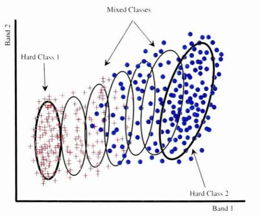
2.3

Illustration

of

the

stochastic

mixing

model

(SMM)

concept

for

a simple

2

class,

2

band

case.

Drawn

are

isoprobability

contours

illustrating

clusters associated with

hard-endmember

classes and mixed pixel classes

19

2.4

Illustration

of

the

convex

hull

as

being

the

minimal convex set encompass

ing

the

data

20

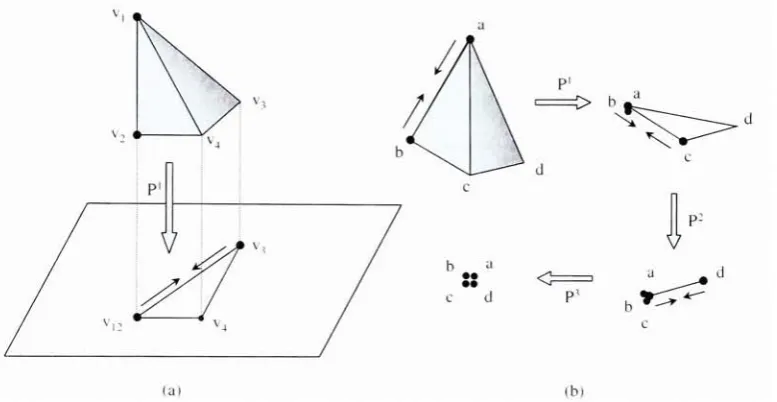
2.5

Illustration

of

(a)

the

preservation ofvertices ofa simplex

through

projec

tion

ofa

data

set onto

the

difference in

two

verticesof a simplex and

(b)

the

conceptof maximum

distance

determination

and sequential projection

to

find

the

vertices of a simplex

spanning

the

data

space

24

2.6

Normalized HYDICE

spectra

for

panel made of green cotton

fabric. The

solid

line

represents

the

spectral radiance of

the

panel

in

direct

sunlight while

the

dotted

red

line

shows

illumination

effectswhen

the

panelwas

in

the

shade

37

2.7

False

alarms

(yellow

pixels)

when

finding

the

F3

spectrum as measured

in

direct

sunlight

in

an

image

where

the

(same)

panel

is

placed

in

the

shade.

The SAM

algorithmwasused

(in

radiance

space)

with a

threshold

of

0.26

radians.

The

white circle arearefers

to the

location

of

the

F3

target

in

the

shade.

Notice

no

detects in

this

region

38

2.8

Average

error as a

function

ofnumberof

basis

vectors

[14]

42

2.9

Experiment in

whicha spectrometer

is

pointed

in

the

direction

of

the

Sun. Black line is

the

normalized radiance

in

the

absence of a cloud

while subsequent measurements arerepresentative of a cloud

passing

in

front

of

the

Sun

46

2.10

Illustration

of spectral matched

filter

(SMF)

parameters

in 3

bands

of an

MNF

space.

The background data has

covariance

A

while

the target's

covariance

is

the

identity

I,

since

target

variability

was

strictly based

on noise

in

the

original space.

The

target

location

relative

to

the

background

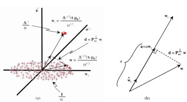
2.11 Illustration

of

SMF

in

normalized whitenedw-space.

(a)

Shows

the

projec

tion

of a sample pixelwonto

the target

vector

wt to

yield

the

abundance

a.

We

also

illustrate

the

orthogonalprojection

d.

Additionally,

the

back

ground

data

now

has

the

covariance of a scaled

identity

matrix

(circular

distribution)

while

the target

data

covariance

is

a scaled version of

the

diagonal

background

data,

(b)

Illustrates

the

quantities associated with

the

abundance

in

more

detail

53

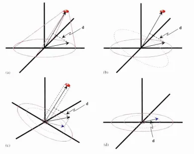
2.12

(a)

Geometric

cone

formed

by

target

and

background data,

(b)

Rotation

and

(c)

projection of

the target

and

background

data

in (a),

(d)

The

projected

d

vector

55

2.13

(a)

Cone

and contour

lines defined

by

s which

is

a

function

of

a,a(t)

and cr(b).

(b)

Illustration

of

two

samples

pixels, wi

and

W2,

with

different

abundances

but

the

same magnitudes

for

the

d

vectors.

However,

the

infeasibility

will

be

greater

for

pixel

1

than

pixel

2

57

3.1

Atmospheric

carbon

dioxide

mixing

ratios

determined from

the

continuous

monitoring

programsat

the

4

NOAA

CMDL baseline

observatories

[18].

.

64

3.2

Absorption

spectra of

(a)

H20,

(b)

03,

(c)

CO,

(d)

C02,

(e)

CH4,

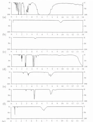
(f)

N20,

and

(g)

O2

as a

function

ofwavelength

\jj.m].

We

can see

that

of all

the

atmospheric

constituents,

H2O is

the

largest

contributor

to

absorption.

66

3.3

MODTRAN

atmospheric water vapor profiles

for

the

first

10 km

of

the

atmosphere

68

3.4

Process

ofobtain

MODTRAN

water vaporscale

factors

using

results

from

physics-based water vaporestimation routines

70

3.5

Illustration showing

the

difference between

the

zenithangle

a'

and

target

3.6

Illustration

of shape

factor

conceptwhere

target

is

not

completely

exposed

to the

hemisphere

above

due

to

anobscurationsuch as a

tree, for

example.

73

3.7

Illustration

of

background

mixing

model as applied

to test

pixel x.

(a)

The

test

pixelxproduces an errorvectore ofzero

because

the

background

model provides a good

fit. Thus

the

pixel

is

very

background-like making

the

abundancea zeroaswell,

(b)

The background

model

is

less

appropriate

for

test

pixel x.

The large

error

implies

the test

pixel

is

not

background-like

which can produce a

larger

projections onto

the target

vector

producing

significant abundances

76

3.8

Illustration

of a possible

false

positive

using

a matched

filter.

In

(a)

the

image

pixel x

is

close

to

the target

andresults

in

an abundancevector a.

In

(b), however,

it is

questionable as

to

whether

the

image

pixel

is

close

to

the target

even

though

it

produces

the

same abundance-like value as

in

(a).

79

3.9

Illustration

of

the

structured

infeasibility

concept as

hyper-cones.

For

simplicity

here,

weassume

the target

space

is

a singlevector

(i.e.,

T

=>

t).

(a)

The

projection of apixel xonto

the

background B

producesvector e

which

is

then

projected onto

target

t to

produce an abundance-likevector

a.

Additionally,

we can generate a vector projection orthogonal

to the

target

termed

d.

(b)

Shows

that

wecan get

the

same abundancevector

for

a "family" of possible

pixels,

all of

which,

however,

have

different

d

values,

which we can

take

advantage of

in generating

a structured

infeasibility

3.10

Illustration

of

2

dimensional

decision

map.

In

(a)

the

most probable

tar

get pixels are

those

with

large

abundances and small

infeasibilities

(SIP

values).

In

(b)

we show

the

expectedstatistical

behavior

of

the

SIP

values

as a

function

of

target

abundance

81

3.11

150

x

250

subset

from

the

larger FR

I,

phase

I,

fully

exposed

data

set. . .

83

3.12

250

x

300

subset

from

the

larger FR

I,

phase

III,

fully

concealed

data

set.

84

3.13

Peak

normalized radiance spectrum

showing

regions

(in

red)

where

data

wasomitted

leaving

170

working

bands

86

3.14 Sub

section

(150

x

250)

of

HYDICE FR I

exposed

image showing locations

and

labeling

of

target

panels.

The

magenta pixels are associatedwith

full

pixelswhile

the

red pixels

denote

sub pixel

targets.

The

yellowpixels are referred

to

as "guard" pixels and are not considered

target

pixels

86

3.15 Sub

section

(250

x

3000)

of

HYDICE FR I

fully

concealed

image showing

locations

and

labeling

of

target

panels.

For

this

research we attempt

to

find

the

F3

panel which

is denoted

by

the

red andyellow pixels

87

3.16

Plot showing ELM'ed derived

reflectances

for

various

targets that

look

similar

to that

ofpanel

F3. It

can

be

seen

that

panel

F5 is

most similar

to

F3,

though

slightly

reduced

in

magnitude

88

4. 1

General location

of collection site

(middle

right of

image)

relative

to

Bal

timore,

MD

95

4.2

Variation in

visibility,

as seen

by

the sensor,

using

a rural extinction model.

The

radiance spectra

include

the target

(F3)

reflectance and are

for

a

fixed

elevation,

water vapor scale

factor,

and

TOD

factors

for

the

fully

4.3

Variation

in

visibility,

as seen

by

the sensor, using

a urban extinction

model.

The

radiance spectra

include

the target

(F3)

reflectance and are

for

a

fixed

elevation and watervaporscale

factor,

and

TOD factors

for

the

fully

exposed collect

98

4.4

Variation in

visibility,

as seen

by

the sensor,

using

amaritime extinction

model.

The

radiance spectra

include

the target

(F3)

reflectance and are

for

a

fixed

elevation andwater vaporscale

factor,

and

TOD

factors for

the

fully

exposed collect.

We

see

the

same

trends

aswith

the

rural extinction

modelexcept

for

much more

scattering

98

4.5

Variation in

the

ground

topography

parameter as configured

in

MOD

TRAN. The

sensor

height is 1.56 km.

We have additionally factored in

variation

due

to

scene elevation of

50

feet

101

4.6

Variation in

sensor

reaching

radianceas

the

ground

topography

parameter

is

altered

(H2).

For

this

plot we

fixed

the visibility to

be 20

km,

used a

ruralextinction

model,

and set

the

sensor

height

to

1.56

km

102

4.7

Plot showing

variation

in

sensor

reaching

radiance as a

function

ofwa

ter

vaporscale

factor.

Atmospheric

model used was

that

of mid-latitude

summer with a

visibility

of

30

km

103

4.8

Estimation

of per pixel

total

column water vapor

using

the

FLAASH

al

gorithm

104

4.9

Histogram

ofwater vapor

map

produced

by

the

FLAASH

algorithm. . . .

105

4.10

Plot

showing the

linear

dependence

of water vapor scale

factor

to total

4.11

(a)

Illustrates

a

180

vector

target

space generated

for

the

fully

exposed

imagery

while

(b)

shows a

180

vector

target

space

for

the

fully

concealed

imagery. Over

plotted

in

both

target

spaces

is

anactual

image derived

F3

target

pixel

112

4.12

(a)

Plot showing

absolute calibration correction

factor

(red

line)

and

the

result of

multiplying

such a correction

factor

to

an

F3

pixel

in

the

fully

concealed

imagery,

(b)

Shows

the

same

target

space

in

Figure

4.11(b)

except with

the

calibrated

F3

pixel over plotted onto

the

fully

concealed

target

space

113

4.13

Estimation

of

target

image

pixel

using

physically derived

target

vectors

for

the

(a)

exposed and

(b)

fully

concealed

data

sets

115

4.14

Plotting

the

reflectance normalized

difference between

the target

image

pixeland

target

pixelestimate

using

physics

based modeling for both

the

(a)

exposed and

(b)

concealed

data

sets

115

4. 15

Cumulative RMS

erroras a

function

ofwavelength

for both

the

(a)

exposed

and

(b)

concealed

data

sets.

The

last

value

in

these

plots

is

the total

RMS

error

116

4.16

Plot

showing

7

endmembers extract

from

the target

spaces generated

for

the

(a)

fully

exposed and

(b)

fully

concealed

image

data

sets

117

4.17

Target labeled FR I

exposed

image.

The

targets

are

in

columns,

above

and

below

each

label

121

4.18

Results

after

applying the

SAM

algorithm

to the

FR

I

exposed

data

set.

The

raw

test

statistic

image

(a)

(map

of

angles)

can

be

seen next

to

a

4.19

Results

after

applying

the

SMF

algorithm

to

the

FR I

exposed

data

set.

The

raw

test

statistic

image

(a)

can

be

seen next

to

a version with a

threshold

applied

(b)

.

For

the

SMF

algorithm

high

values

(bright

pixels)

are equivalent

to the

most probable

detects

124

4.20 Results

after

applying

the

PBosp

algorithm, using

7

basis

vectors, to the

FR I

exposed

data

set.

The

raw

test

statistic

image

(a)

can

be

seen next

to

a versionwith a

threshold

applied

(b).

For

the

PBosp

algorithm

high

values or abundances

(bright

pixels)

are equivalent

to the

most probable

detects

125

4.21

Results

after

applying

the

PBosp

algorithm, using the

mean

target

space

vector, to the

FR I

exposed

data

set.

The

raw

test

statistic

image

(a)

can

be

seen next

to

a versionwitha

threshold

applied

(b). For

the

PSosp

algorithm

high

values or abundances

(bright

pixels)

are equivalent

to the

mostprobable

detects

126

4.22 ROC

curves

for

the

SAM, SMF, PBosp

algorithms,

as applied

to the

FR I

exposed

data

set.

The SAM

and

SMF

algorithms used

ELM data. Shown

are results plotted

using

(a)

linear

and

(b)

log

scales.

For

the

log

scale

in

(b),

the

curves start

from

the

left

when

the

detector

encounters

the

first

false

alarm

(FA). That

is,

since

there

is

no

"zero",

the

curves appear

(or

start)

when

the

detector

encounters a

FA. For

the

PBospjmean case,

the

first FA is

encountered around

2.5

10~2

4.23 ROC

curves

for

the

SAM, SMF, PBosp

algorithms,

as applied

to the

FR

I

exposed

data

set.

The SAM

and

SMF

algorithms used

ATREM data.

Shown

are results plotted

using

(a)

linear

and

(b)

log

scales.

For

the

log

scale

in

(b),

the

curves start

from

the

left

when

the

detector

encounters

the

first false

alarm

(FA)

130

4.24

ROC

curves

for

the

SAM, SMF, PBosp

algorithms,

as applied

to the

FR

I

exposed

data

set.

The SAM

and

SMF

algorithms used

FLAASH data.

Shown

are results plotted

using

(a)

linear

and

(b)

log

scales.

For

the

log

scale

in

(b),

the

curves start

from

the

left

when

the

detector

encounters

the

first

false

alarm

(FA). That

is,

since

there

is

no

"zero",

the

curves appear

(or

start)

when

the

detector

encounters a

FA

131

4.25

Target labeled

subsection

(250

x

300 pixels)

of

the

larger FR I

concealed

image

132

4.26

Results

after

applying

the

SAM

algorithm

to the

FR I

concealed

data

set.

The

raw

test

statistic

image

(a)

(map

of

angles)

can

be

seen next

to

a version with a

threshold

applied

(b).

For

the

SAM

algorithm

low

values

(dark

pixels)

areequivalent

to the

most probable

detects

134

4.27

Results

after

applying

the

SMF

algorithm

to

the

FR I

concealed

data

set.

The

raw

test

statistic

image

(a)

can

be

seen next

to

aversionwith a

threshold

applied

(b).

For

the

SMF

algorithm

high

values

(bright

pixels)

4.28 Results

after

applying

the

PBosp

algorithm,

using 7 basis

vectors, to the

FR

I

concealed

data

set.

The

raw

test

statistic

image

(a)

can

be

seen next

to

a versionwith a

threshold

applied

(b).

For

the

PBosp

algorithm

high

values or abundances

(bright

pixels)

are equivalent

to the

most probable

detects

137

4.29 Results

after

applying

the

PBosp

algorithm,

using

the

mean

target

space

vector, to the

FR

I

concealed

data

set.

The

raw

test

statistic

image

(a)

can

be

seennext

to

aversion with a

threshold

applied

(b). For

the

PSosp

algorithm

high

values or abundances

(bright

pixels)

are equivalent

to the

most probable

detects

138

4.30

ROC

curves

for

the

SAM, SMF, PBosp

algorithms,

as applied

to

the

FR I

concealed

data

set.

Shown

areresultsplotted

using

(a)

linear

and

(b)

log

scales

140

4.31

HYDICE image

used

to

obtain sensor noiseestimate.

A 1000

sampleregion over

water,

located in

the

lower

left

of

the

image,

wasused

to

as

input

to

ENVI's MNF

procedure

142

4.32

(a)

Shows

the

2 dimensional

correlation matrix of

the

noise statistics

file

associated with

the

water region while

(b)

illustrates

the

sharp fall

off

in

variance associated with

the

first 10 MNF

bands,

as applied

to the

ELM'ed

4.33

Infeasibility

results

from ENVI's

MTMF

algorithm as applied

to the

FR

I

exposed

data

set compensated with

ELM.

Here,

we

have

keep

all

MNF

bands.

The

raw

test

statistic

image

(a)

can

be

seen next

to

a version

(b)

with a

threshold

applied, showing

the

first

1500

scores.

For

the

INF

algorithm

high

values

(bright

pixels)

are equivalent

to

large

infeasibility

values

145

4.34

Infeasibility

results

from

ENVI's MTMF

algorithm as applied

to the

FR I

exposed

data

set compensated with

ELM.

Here,

we used

the

first 8 MNF

bands.

The

raw

test

statistic

image

(a)

can

be

seen next

to

a version

(b)

with a

threshold

applied, showing

the

first

1500

scores.

For

the

INF

algorithm

high

values

(bright

pixels)

are equivalent

to

large

infeasibility

values

146

4.35

Infeasibility

results

from ENVI's MTMF

algorithm as applied

to the

FR

I

exposed

data

set compensated with

ATREM.

Here,

we used

the

first

8

MNF bands. The

raw

test

statistic

image

(a)

can

be

seennext

to

a version

(b)

with a

threshold applied,

showing

the

first

1500

scores.

For

the

INF

algorithm

high

values

(bright

pixels)

are equivalent

to

large

infeasibility

values

147

4.36

Infeasibility

results

from ENVI's MTMF

algorithm as applied

to the

FR

I

exposed

data

set compensated with

FLAASH.

Here,

we used

the

first

8

MNF bands. The

raw

test

statistic

image

(a)

can

be

seen next

to

a version

(b)

with a

threshold applied,

showing

the

first

1500

scores.

For

the

INF

algorithm

high

values

(bright

pixels)

are equivalent

to

large

infeasibility

4.37

Infeasibility

results

from applying

the

SIP

algorithm

to the

FR I

exposed

radiance

data

set.

The

raw

test

statistic

image

(a)

can

be

seen next

to

a version with a

threshold

applied

(b).

For

the

SIP

algorithm

high

values

(bright

pixels)

are equivalent

to

large

infeasibility

values

149

4.38

Infeasibility

results

from ENVI's MTMF

algorithmas applied

to the

FR

I

concealed

data

set compensated with

ELM.

Here,

we

have

keep

all

MNF

bands.

The

raw

test

statistic

image

(a)

can

be

seen next

to

a version

(b)

with a

threshold applied,

showing

the

first

1500

scores.

For

the

INF

algorithm

high

values

(bright

pixels)

are equivalent

to

large

infeasibility

values

150

4.39

Infeasibility

results

from ENVI's MTMF

algorithm as applied

to the

FR

I

concealed

data

set compensated with

ELM.

Here,

we used

the

first

8

MNF bands. The

raw

test

statistic

image

(a)

can

be

seennext

to

aversion

(b)

with a

threshold applied,

showing

the

first

1500

scores.

For

the

INF

algorithm

high

values

(bright

pixels)

are equivalent

to

large

infeasibility

values

151

4.40

Infeasibility

results

from applying

the

SIP

algorithm

to the

FR I

concealed

data

set.

The

raw

test

statistic

image

(a)

can

be

seen next

to

a version

with a

threshold

applied

(b).

For

the

SIP

algorithm

high

values

(bright

pixels)

areequivalent

to

large

infeasibility

values

152

4.41

Two dimensional decision

spaces created

using the

PB-SIFT algorithm,

as

applied

to the

FR I

exposed

data

set.

(a)

Shows

the

result of

using

PB-SIFT,

using the

entire

target space,

(b)

shows

the

result of

using

PB-SIFT,

using

7 basis

vectors,

and

(c)

shows

the

result of

using

PB-SIFT,

using

the

4.42 Two dimensional

decision

spaces created

using

the

MTMF

algorithm,

as

applied

to the

FR

I

exposed

data

set.

(a)

Shows

the

result

using ELM

data

withall

(170)

MNF

kept

while

(b)

only keeps

the

first

eight.

Decision

spaces are also shown

using

(c)

ATREM

and

(d)

FLAASH

compensated

imagery

159

4.43

Two dimensional

decision

spaces created

using

the

PB-SIFT

algorithm,

as applied

to the

FR I

concealed

data

set.

(a)

Shows

the

result of

using

PB-SIFT,

using

the

entire

target space,

(b)

shows

the

result of

using

PB-SIFT,

using 7 basis

vectors,

and

(c)

shows

the

result of

using

PB-SIFT,

using

the

mean

target

space vector

161

4.44 Two

dimensional decision

spaces created

using

the

MTMF

algorithm,

as

applied

to the

FR I

concealed

data

set.

(a)

Shows

the

result

using ELM

data

with all

(170)

MNF kept

while

(b)

only

keeps

the

first

eight

162

4.45 ROC

curve

improvement

using

various

SIP

thresholds,

as applied

to the

FR

I

exposed

imagery.

The

SAM

and

SMF

algorithms were applied

to

ELM

compensated

imagery,

(a)

Shows

ROC

curves

using

a

truth

mask

that

allows

for FA's

on other man-made panels while

(b)

shows an

increased

ROC

performance

for

the

PBosp.bv

case

165

4.46

ROC

curve

improvement using

various

SIP

thresholds,

as applied

to the

FR I

concealed

imagery.

The

SAM

and

SMF

algorithms were applied

to

ELM

compensated

imagery,

(a)

Shows

ROC

curves

using

a

truth

mask

that

allows

for FA's

on other man-made panelswhile

(b)

shows an

increased

4.47 Results from

testing

the

expected

behavior

of

the

Structured

Infeasibility

Projector (SIP).

We

can see

that

as

the target

abundance

in

a

background

pixel

increases,

the

overall variance and mean projected

distance decreases.

169

4.48 Two

dimensional

decision

space created

using the

PB-SIFT

algo

rithm,

as applied

to the

FR I

concealed

data

set.

This

example

3.1

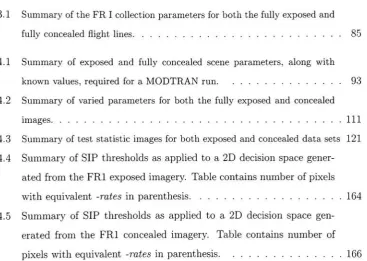
Summary

of

the

FR I

collectionparameters

for both

the

fully

exposed and

fully

concealed

flight

lines

85

4.1

Summary

of exposed and

fully

concealed scene

parameters,

along

with

known

values,

required

for

a

MODTRAN

run

93

4.2

Summary

of varied parameters

for both

the

fully

exposed and concealed

images

Ill

4.3

Summary

of

test

statistic

images for both

exposed and concealed

data

sets

121

4.4

Summary

of

SIP

thresholds

as applied

to

a

2D

decision

space gener

ated

from

the

FRI

exposed

imagery.

Table

contains number of pixels

with equivalent -rates

in

parenthesis

164

4.5

Summary

of

SIP

thresholds

as applied

to

a

2D

decision

space gen

erated

from

the

FRI

concealed

imagery.

Table

contains number of

pixels with equivalent -rates

in

parenthesis

166

[image:30.491.67.435.236.497.2]

to the

gates of

the temple

ofscience arewritten the words:

'Ye

must

have

faith."

Max

Planck

Introduction

1.1

Remote

Sensing

and

Spectroscopy

Remote

sensing,

for

all practical

purposes,

is

the

field

of

study

associated with

extracting information

about an object without

coming

into

physical contact with

it.

A definition

such as

this

can

include

a multitude of

disciplines

such as medical

imaging,

astronomy, vision, sonar,

and earth observation

from

above via an aircraft or space satellite.

For

the

most

part,

remote

sensing is

often

thought

of

in

the

latter

context, viewing

and

analyzing

earth

from

above.

The field

of remote

sensing

is

has been evolving for

over

50

years.

This

goes

back

to the

late 40s

and

early

50s

whensomeof

the

first

satellitephotographs were

being

recovered

from V-2 launches.

During

this

time the

satellite

imaging

of

the

earth

developed hand

in

hand

with

the international

space program.

Following

the

first

manmade satellite

launch

of

Sputnik 1

on

October

4,

1957,

photographs and video

images

were acquired

by

U.S. Explorer

and

Mercury

programs and

the

Soviet Unions

LUNA

series.

Just 3

years after

Sputnik l's debut

(April

1960),

the

U.S. initiated its

spaced-based reconnaissanceprogram

acquiring

high-resolution

photographic

images

from

space

[38].

Today

remote

sensing is

used

in

a

variety

ofapplications such as environmental

mapping,

globalchange

research,

geological

research,

wetlands

mapping,

assessment

of

traceability,

plant and mineral

identification

and abundance

estimation, target

detection

and

classification,

and

crop

analysis.

What

makes

the study

of

these

application areas possible

is

the

fact

that

materials

that

make

up

objects

in

a scene

(i.e.,

vehicles,

wheat

fields,

body

of

water,

etc.)

can

be

characterized

due

to the

fact

that

they

reflect, emit, scatter,

and absorb electromagnetic

(EM)

radiation

differently.

One

can

take

advantage of

this

fact

and

say

that, ideally,

each material

therefore

has

a unique characteristic

feature. If

weare

looking

at

this

interaction in

many

regions of

the

EM

spectrum

then

we go on

to

further

say that

each material

has

a unique spectral signature.

The

analysis and

interpretation

of such spectral

signatures

is

called spectroscopy.

This

material signature

is

usually

propagated

through the

atmosphere where

it

falls incident

on an

imaging

systems sensor.

Today,

most

imaging

system sensors

are of a solid state

design.

This

enables one

to

design

a system

(in

conjunction

with a

dispersing

element)

that

can

simultaneously

capture spatial as well as spec

troscopic

information

about a piece of real estate

below. These

systems are called

imaging

spectrometers and can

be

essentially

divided into

those that

use one

to ten

E fiP i'.

.

,- | i . Pi ..

1 fayI

',,=.

-Figure

1.1:

Overview

of collection capabilities of a

hyperspectral

sensorsystem.

Shown

are materials with

distinctive

spectroscopic characteristics obtained

through the many

band

or channels

the

instrument

collects

[49].

channels

(hyperspectral). An

example of such a system

is

shown

in

Figure

1.1.

The

field

of

imaging

spectrometery

has been

under

development

since

the

1970s

as a means of

identifying

and

mapping

earth resources.

As

a

result,

hyperspectral

data,

in

particular,

permit

the

expansion of

detection

and classification activities

to targets previously

unresolved

in

multispectral

images.

Examples

of such

hyper

[image:33.491.125.385.94.310.2]

1.2

Hyperspectral

Application Areas

Of

the

many

applications

areas

in

remote

sensing,

hyperspectral

remote

sensing

tends to

focus

on

topics

in

three

major

categories,

(i)

anomaly

detection,

(ii)

tar

get recognition and

detection,

and

(iii)

background

characterization.

Anomaly

de

tection

seeks

to

find

signatures of unusual

materials,

as compared

to

background

materials,

without a priori

knowledge

of

the target.

In

contrast, target

detection

algorithmsuse

known information

about a material of

interest

and seek

to

find

such

a

material(s) in

the

scene.

The

a priori

information

may

originate

from

a spectral

library

or

be image derived. In

target recognition,

we not

only detect

the target

(s)

but

we assign

it

a

label

or name.

This

method of

detection is

called classifica

tion.

Classification

is

usually

a name given when one

is

dealing

with

grouping

a

large

number of pixels

into

multiple classes.

For

target

detection,

the

number of

objects one seeks

to

find is

usually very

sparse and man-made

in

nature.

The last

category,

background

characterization,

deals

with

the

characterization of

the

overall

scene

background.

Examples

of

this

include,

terrain categorization,

water

quality

assessment,

atmospheric

compensation,

and plume

detection

and quantification.

In

this research,

we

focus

on

the

development

of

target

detection

algorithms

that

use

hyperspectral

data

captured with

imaging

spectrometers.

1.3

Hyperspectral

Target Detection:

Considerations

There

are

many

issues

that

cancomplicate

the

success oroutcomeof

the

above men

tioned

algorithms.

One

such

issue is

atmospheric compensation.

In

most

cases,

one

atmospherically

compensates

imagery

to

ground

leaving

reflectance

before applying

interest is usually

measured

in

reflectance units.

In

this

case

the

success of

the

de

tection

algorithm

is

highly

dependent

on

the validity

of

the

compensation algorithm.

The

method and

type

of compensation

is

a significant part of

hyperspectral

remote

sensing

and

is

the

subject of

ongoing

research.

In

this

research we will

be

taking

the

approach of

developing

and

applying

algorithms on uncompensated

imagery.

Rather

than

"back

out"

the

atmosphere

to

gain access

to the

ground reflectance

target

spectrum we

simply

propagate

the target through the

atmosphere

using

a

physics

based

model and generate a probabilistic

target

space

that

resembles what

the target

might

look like

as seen

by

the

imaging

sensor.

That

is,

a

target

sensor

reaching

radiance space

is

developed

that

can

be

used

in

a

detection

scheme.

Another issue

that

needs

to

be

considered

is

variability

in

the

data.

In

general,

materials

in hyperspectral data

do

not exhibit

deterministic behavior.

Rather,

a single material will exhibit a

fair

amountof random

variability that

needs

to

be

ac counted

for in

the

detection

model.

The

variability

can arise

from

poor atmospheric

compensation,

spectrometer

instrument

error,

sensor

noise,

self

shadowing,

adja

cency

effects and geographic

location.

Additionally,

variability

can arise

from

nat ural variation

in

the target

or

variability

due

to

lack

of specific

knowledge

about

the

target.

The

most popular

techniques to

characterize

this variability

involve

either vector algebra

(geometry)

or statistical

descriptors.

In

the

geometric sense we use

endmembers,

whereas means and covariances are used as statistical

descrip

tors.

Examples include

probability

density

(statistical)

and

(linear)

mixing

models

(geometric).

Lastly,

there

is

the

issue

of

full

versus mixed pixels.

Depending

on

the

sensor

ground resolved

distance

(GRD),

pixels will either

be 100%

filled

or

partially

filled

appropriatemodel.

1.4

Research Overview:

Work

Statement

Most detection

models are

based

on

the traditional

matched

filter

and

describe

the

background

variability

through

use of geometric or stochastic means.

This

research

explores

the

development

of ageometricalgorithm

that

factors in

a

physically

based

target

model

to

account

for

target variability

while

using

an additional metric

that

aids

in rejecting

false

alarms.

This

geometric approach

is

very

similar

to

the

sto

chastic

Mixture Tuned Matched Filter

(MTMF)

which uses a spectral matched

filter

and an

infeasibility

metric

to

reduce

false

alarms.

An

overview of

the

research

into

physics

based modeling

and algorithm

development is

provided

below.

Full

literature

search and overview of relevant concepts and methods as

they

relate

to

physics

based modeling

and

target

detection.

Improved

physics

based

modeling

of a

target

space.

This includes investigation

on what parameters

to

use when

generating

a

target space,

how

they

are

used,

and what values are appropriate when

using them.

Incorporate

improvements to

current usage of physics

based

modeling.

This

includes

any

modifications

to the sensor-reaching

radiance equation.

Develop

a new

(hybrid)

detector

that

can utilize results

from

physics

based

modeling.

Develop

ageometric equivalent

to the

infeasibility

concept.

Develop

a newgeometric

detector

that

is based

on

the

MTMF.

Explore

the

behavior

of

2D detector

spaces.

Compare

results of new physics

based detectors

to the

Spectral

Angle

Map

"The fewer

the

facts,

thestronger

the

opinion."

Arnold

H.

Glasow

Background

In

this

background

section we

describe

many

of

the

approaches used

in

traditional

target

detection.

We

start off with an explanation of signal

detection

theory

and

how it

relates

to target

detection

through

development

of

the

hypothesis

test.

This

leads

us

to the

derivation

of

the

likelihood

and generalized

likelihood

ratio

tests.

We

then

explore methods

to

characterize

background

spaces

in

a stochastic sense

followed

by

appropriate statistical models.

This is

a segue

into

geometrical

(end-members)

methods

to

characterize

the

background

followed

by

a

description

of

the

linear

mixing

model.

Subsequent

sections

describe

approaches

to target

detection

(both

in

a geometric and statistical

sense) for

fully

resolved and mixed pixels.

We

then introduce the

concept of

target

spaces and physics

based modeling

al-gorithm.

Finally,

we

introduce hybrid

algorithms

that take

advantage of statistical and

geometric

descriptors.

2.1

Signal Detection

Theory

Detection

theory

is

a generalized

term

used

to

categorize

decision making

about whether or not a particular event occurs.

For

example,

in

radar one might

be

interested in

determining

the

presence or absence of an

approaching aircraft,

which

may

be

obscured

by

background

noise.

Here

we choose

between

two

possible cases

in seeking

out

the

aircraft:

(i)

the

aircraft and noise are present or

(ii)

noise

only

is

present.

This decision making

process can

be

thought

of as a

binary

hypothesis

testing

problem.

If

the

nature of

the

data is

random,

with noise as an

example, then

a statistical approach

is

necessary.

Here,

the

binary

hypothesis

testing

problem

turns

into

a statistical

hypothesis

testing

problem.

The

typical target

detection

chain

that

creates such

binary

detection

maps can

be

seen

in Figure 2.1.

In

general, the

simplest

detection

problem

is

one

that

involves

a

known determin

istic

signal andcontains

background

noise

that

is

Gaussian

with a

known probability

density

function (PDF). The

problem

becomes

more

difficult

as

the

deterministic

signal

becomes

random with an unknown

distribution

and

the

Gaussian

assumptions

become

non

Gaussian

with unknown

PDF's. These latter

conditionsall

decrease de

tection

performance

due

to the

fact

that

less is known

about

the

characteristics of

Target

*

Detection

Algorithm

Detection

Map

Target Spectra

Figure 2.1:

Typical

target

detection

process

showing

a

detection

map

for

the

3 input

target

spectra.

2.1.1

Hypothesis

Testing

and

the

Likelihood Ratio

(LR)

Lets

say

we are given an observed pixel spectrum x such

that

xT

=

[.r(A1),x(A2),---,x(Ap)]

(2.1)

for

p-spectral

bands

and we wish

to

decide if

the

pixel

has

an

interesting

"target"

in it.

Given

this situation,

we establish

the

following

binary

hypothesis

test

for

the

pixel:

34o:

target

absent

"Ky.

target

present

where

Jio

is

referred

to

as

the

null

hypothesis

and

"Hi

as

the

alternative

hypothesis.

For

illustrative purposes,

we present a univariate example of

this

binary

hypothesis

test.

If

we assume x

is

a realization of a multivariate

Gaussian

random

variable,

then

we will assume

the

PDF

of x

from

a single

band

comes

from

either

N(ji0,a2)

p(x;

%)

p(x;

X,)

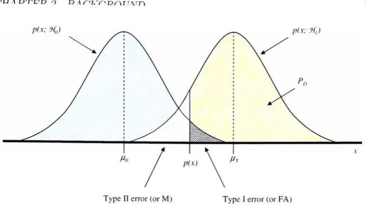
[image:41.491.68.435.68.273.2]

Type II

error(or

M)

Type I

error(or

FA)

Figure 2.2:

Probability density

functions

for

hypothesis

testing

problem

showing

errors

and

probability

of

detection

Pq

.

In

the

event

that

we

decide

Jfi

(target

present) but

-K0

is

true

(target

is

actually

absent),

we make what

is

called a

Type I

error.

This is

typically

termed

a

false

alarm

(FA)

by

engineers.

On

the

other

hand,

if

we

decide

!K0

but

!Ki

is

true,

we make a

Type II

error.

The engineering

community

refers

to this type

of error as a miss

(M)

(cf.

Figure 2.2). In

general,

it

is

well

known

that

detectors based

on

the

likelihood

ratio

(LR)

test

have

certain advantages over analysis of

the probability

functions

individually

[33].

The LR

minimizes

the

risk associated with

incorrect decisions

as

wellas

leads

to

detectors

that

are optimum

for

a wide range ofperformancecriteria.

This

ratio

is

usually

defined

as

C(x)

p(x;

"Ki

(2.2)

p(x;

_H0)

'

If

(x)

exceeds a

threshold

7, then the

alternative

hypothesis

(target

present) is

detector

or

detection

statistic,

the

former

of which

is

a

label

used

by

the engineering

community

[23].

If

the

probability

density

functions

in

Eq.

(2.2)

are

completely

known,

then

the test

is

called a simple

hypothesis

test.

In

the

event

that the

PDF's

are not

completely

known,

then

we

have

what

is

called a composite

hypothesis

test.

2.1.2

The Neyman-Pearson Approach

It is

always of great

desire

to

select

the threshold 7,

such

that

one maximizes

the

number of correct

detections

while

minimizing the

numberof

target

misses and

false

alarms.

In

the

event

that

we

have

a simple

hypothesis

test

wecan choose a

threshold

based

on either

the

Neyman-Pearson

theorem

or

the

Bayesian

approach,

which

is

based

on minimization of

the

Bayes

riskmost often seen

in

classification problems.

In

the

later,

we choosea

threshold that

leads

to

minimize

both false

alarms

(FA)

and

misses

(M).

However,

in

detection

applications,

where

the probability

of occurrence of a

target

is

very small,

minimization of

the

error

probability

(FA

and

M)

is

not a good criterion of

performance,

because

the probability

of error can

be

minimized

by

classifying

every

pixel as

background

[33]

.

A better

approach

is

to

maximize

the

probability

of

choosing

"K\

when

indeed

it is

true

(detection),

while not

exceeding

a

"fixed"

probability

of

choosing

"K\

when

it

is

false

(false

alarm).

This

approach

is

called

the Neyman-Pearson theorem

[23]

which

simply

maximizes

the

probability

of

detection

(Pd)

given a

fixed

value a

for

the probability

of

false

alarms

(Pfa)-Therefore,

we

decide

"K\,

for

a given

PFA

a,

if

t(x)

=

When working

with remote

sensing

data

typical

per-pixel values

for

a range

from

IO"4

to

IO"6.

2.1.3

Generalized Likelihood

Ratio

In practice, information

about

the

PDF's

under

the two

hypotheses

(3f0

and

%{)

may

not

be known.

In

this

case we cannot use

the

Neyman-Pearson

method

de

scribed above.

Instead,

we replace

the

unknown parameters

in

Eq.

(2.3)

with

their

maximum

likelihood

estimates

(MLE).

This

approach

is

called

the

generalized

like

lihood

ratio

(GLR)

test

and produces a

family

of,

what are

typically

called,

adaptive

detectors.

These detectors

are

termed

adaptive

because

the

unknown parameters

must

be

estimated

from

the

actual

image data.

2.2

Estimation

of

Target

and

Background

Spaces

In

the

previous section we

introduced

the

concept of a

likelihood

ratio

based

on

the

Neaman-Pearson

criteria.

If

the

distributions in

the two

hypotheses

contain

unknown

parameters, then the

detector

was

termed

"adaptive" and called a gener

alized

likelihood

ratio

test.

In

this case, the

unknown parameters must

be

estimated

from

the

background

or

target

space.

There

are

many techniques

in estimating

these

parameters all of which

depend

on

the

type

of

detection

model used.

If

the

model

requires means and covariance's

then

a statistical approach

is

necessary.

However,

if

we use a subspace or

mixing model, then the

matrices

in

the

model are

usually

2.2.1

Stochastic Methods

More

often

than not,

weare

trying

to

characterize

background

(or

target)

variability

due

to

effects such as

atmospheric

conditions, noise,

or

variability

in

the

material

itself. In

the

event

that the

background

or

target

does

not

vary

(i.e.,

is

determinis

tic)

then there

would

be

no need

for

characterization of

targets

or

background

via

stochastic methods.

This is usually

not

the

case.

There

are

many different

ways

to

characterize

these target

and

background

spaces,

some of which are

discussed below.

Local

(Windowing)

and

Global Approaches

A

straight

forward

approach

to

c