Development and application of lattice Boltzmann method for complex axisymmetric flows

Development and Application of Lattice Boltzmann

Method for Complex Axisymmetric Flows

Thesis submitted in accordance with the requirements of the

University of Liverpool for the degree of Doctor in Philosophy

by

Wei Wang (BEng

,

MSc)

i

Abstract

ii

iii

I would like to express my sincere thanks to my supervisor, Dr. Jian Guo Zhou, for his encouragement, guidance and support to me throughout the PhD project. His patience, motivation, enthusiasm and immense knowledge not only helped me in all stages of the research and writing up of the PhD thesis, but also set an example that I aim to achieve some day.

It has been a pleasure to share time with my office mates, Li Yaru, Yin Yue, Zheng Peng and Li Xiaorong for their helpful discussions and enjoyable time during the long hours in the office.

My deepest gratitude goes to my parents, my wife and my daughter who are the source of my strength. Without their encouragement, understanding and love, it would have been impossible for me to complete this work.

iv

Publications

1. W. Wang and J. G. Zhou. Lattice Boltzmann Method for Axisymmetric Turbulent Flows. International Journal of Modern Physics C,26(9): 1550099, 2015.

2. W. Wang and J. G. Zhou. Enhanced Lattice Boltzmann Modelling of Axisymmetric Flows. Proceedings of ICE: Engineering and Computational Mechanics, 167: 156-166, 2014.

v

Abstract ... i

Acknowledgement ... iii

Publications ... iv

Contents ... v

List of Figures ... viii

List of Tables ... xii

List of Abbreviations and Symbols ... xiii

Chapter 1: Introduction and Literature Review ... 1

1.1 Background ... 1

1.2 Lattice Gas Automata ... 3

1.3 Lattice Boltzmann Methods ... 5

1.4 Axisymmetric Lattice Boltzmann Method (AxLAB®) ... 6

1.4.1 Study of Pulsatile Flow ... 8

1.4.2 Study of Rotation Flow ... 10

1.4.3 Study of Turbulent Flow ... 13

1.5 Aims and Contributions ... 14

1.6 Outline of the Thesis ... 15

Chapter 2: Governing Equations for Axisymmetric Flows... 17

2.1 Introduction ... 17

2.2 The Navier-Stokes Equations ... 17

2.3 Governing Equations in Axisymmetric Flows ... 19

2.3.1 Laminar Flow ... 19

2.3.2 Turbulent Flow ... 20

Chapter 3: Lattice Boltzmann Method ... 26

vi

3.2 Derivation of the Lattice Boltzmann Equation ... 26

3.2.1 Relation to Continuum Boltzmann Equation ... 29

3.3 Lattice Pattern ... 31

3.4 Local Equilibrium Distribution Function ... 33

3.5 Lattice Boltzmann Equation for Axisymmetric Flows ... 37

3.5.1 Axisymmetric Flows without Swirl ... 37

3.5.2 Recovery of the Axisymmetric Flow Equations without Swirl ... 39

3.5.3 Axisymmetric Flows with Swirl ... 45

3.5.4 Recovery of Axisymmetric Lattice Boltzmann Equation with Swirl ... 47

3.6 Stability conditions ... 50

Chapter 4: Simulation of Non-Newtonian Fluids ... 52

4.1 Introduction ... 52

4.2 AxLAB® for non-Newtonian Fluids Simulation ... 52

4.3 Recovery of the Axisymmetric Flow Equations for non-Newtonian Fluids... 54

Chapter 5: Large Eddy Simulation for Turbulent Flows ... 60

5.1 Introduction ... 60

5.2 AxLAB® with the Subgrid-Scale Stress Model (SGS) ... 61

5.3 Recovery of the AxLAB® with Turbulence ... 64

Chapter 6: Initial and Boundary Conditions ... 71

6.1 Introduction ... 71

6.2 Solid Boundary Conditions ... 71

6.2.1 No-slip Boundary Condition ... 71

6.2.2 Slip Boundary Condition ... 72

6.2.3 Semi-slip Boundary Condition ... 73

6.3 Inflow and Outflow Conditions ... 74

6.4 Periodic Boundary Condition ... 76

6.5 Initial Condition ... 77

6.6 Solution Procedure ... 77

vii

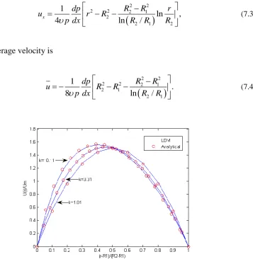
7.2 Flows through a Concentric Annulus ... 80

7.3 Steady Flow through a Constricted Pipe ... 82

7.4 Steady Flow through an Expanded Pipe ... 85

7.5 Unsteady Tube Flow (3D Womersley Flow) ... 88

7.6 Cylindrical Cavity Flow ... 91

7.7 Different Forced Axisymmetric Laminar Cold-Flow Jets... 94

7.7.1 Low-Amplitude Forced Flow ... 95

7.7.2 High-Amplitude Forced Flow ... 96

7.8 Swirling Flow in a Cylinder with Rotating Top and Bottom ... 101

Chapter 8: Applications to non-Newtonian Fluid Flows ...109

8.1 Introduction of Taylor Couette Flow ... 109

8.2 Simulation to Newtonian and non-Newtonian Fluid Taylor Couette Flow .... 109

Chapter 9: Applications to Turbulent Flows ...116

9.1 Flows through an Abrupt Axisymmetric Constriction ... 116

9.2 Axisymmetric Separated and Reattached Flow ... 120

9.3 Pulsatile Flows in a Stenotic Vessel ... 123

Chapter 10: Conclusions and Future Work ...126

10.1 Introduction ... 126

10.2 Conclusions ... 126

10.3 Future Research ... 128

viii

List of Figures

Figure 1.1 Lattice for FHP model. ... 3

Figure 2.1 Cartesian coordinate system. ... 18

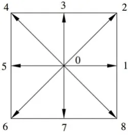
Figure 3.1 Nine-speed square lattice (D2Q9). ... 26

Figure 3.2 Lattice Patterns: 9-speed square lattice (D2Q9) and 7-speed hexagonal lattice (D2Q7). ... 31

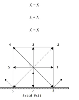
Figure 6.1 Layout of no-slip boundary conditions. ... 72

Figure 6.2 Slip boundary condition layout. ... 73

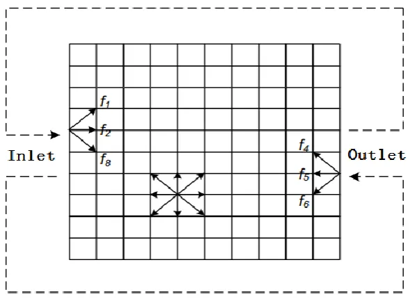
Figure 6.3 Sketch for inflow and outflow boundaries. ... 75

Figure 6.4 Sketch for the Periodic Boundary Condition ... 77

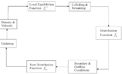
Figure 6.5 Flow chart to demonstrate the LBM calculation procedure. ... 78

Figure 7.1Velocity vectors for steady flow through a straight pipe by AxLAB®. ... 79

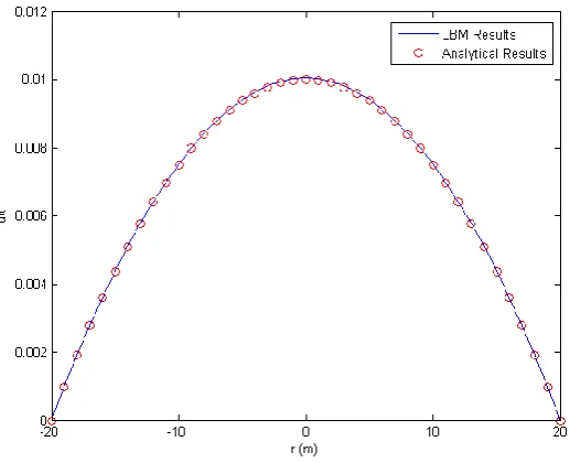
Figure 7.2 Velocity U_x distribution across cross section in pipe flow ... 80

Figure 7.3 Flow through a concentric annulus. ... 80

Figure 7.4 Velocity profile for flow through concentric annulus with radius ratio 1.01, 3.31 and 10.11. k  ... 81

Figure 7.5 Velocity vectors when k3.31 by AxLAB®. ... 81

Figure 7.6 Geometry of constricted pipe. ... 82

ix

Figure 7.9 Radial velocity profiles in constricted pipe for different constriction

radial heights. ... 85

Figure 7.10 Geometry of expanded pipe. ... 85

Figure 7.11 Velocity vectors when  R/ 2. ... 86

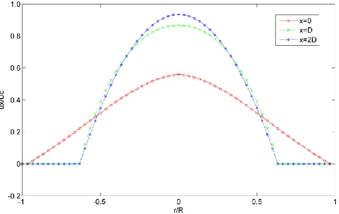
Figure 7.12 Axial velocity profiles in expanded pipe at different distances when / 2. R   ... 87

Figure 7.13 Radial velocity profiles in expanded pipe at different distances when / 2. R   ... 87

Figure 7.14 Axial velocity profiles in expanded pipe at x0, compared with two time steps 0.5t and 2t, when  R/ 4. ... 88

Figure 7.15 Comparisons when u_x is increasing at different timestnT/16, with n=0, 1, 2, 3, 12, 13, 14, 15. ... 90

Figure 7.16 Comparisons when u_x is decreasing at different times, tnT/16, with n=4, 5, 6, 7, 8, 9, 10, 11. ... 90

Figure 7.17 Definition sketch for cylindrical cavity flow. ... 91

Figure 7.18 Stream lines for Case (a) with  = 1.5 and Re = 990. ... 92

Figure 7.19 Stream lines for Case (b) with = 1.5 and Re = 1290. ... 92

Figure 7.20 Stream lines for Case (c) with A = 2.5 and Re = 990. ... 93

Figure 7.21 Stream lines for Case (d) with A = 2.5 and Re = 1290. ... 94

Figure 7.22 Wall jet forced flow. ... 94

Figure 7.23 Centreline velocities for steady jets and amplitude A = 10% forced laminar jets; steady jets are compared with data from Barve et al. ... 96

x

Figure 7.25 Centreline velocities against distance for 200% amplitude forcing. ... 101 Figure 7.26 Comparison of time-averaged centreline velocities with the solution

of Barve et al. at 200% amplitude forcing. ... 101 Figure 7.27 Sketch of the flow geometry. ... 102 Figure 7.28 Diagrams of oscillatory instability in a cylinder with rotating top and counter-rotating bottom,  2... 103 Figure 7.29 Streamlines for counter-rotating cylinder at different Reynolds

number  0.51: (a) Re=3000, (b) Re=2200. ... 104 Figure 7.30 History of the axial velocity at point(x0.25 , H r0.5 )R . ... 104 Figure 7.31 Stream lines for unsteady swirl flow in a cylinder with

counter-rotating bottom at Re=3250, and   0.52. Four different times in a period (a) tt₀ (b) t t₀ T/ 4 (c) t t₀ T/ 2 (d) t t₀ 3 / 4.T ... 105 Figure 7.32 Diagrams of oscillatory instability in a cylinder with rotating top and co-rotating bottom,  2. ... 106 Figure 7.33 Streamlines for co-rotating cylinder at different Reynolds number

and ratio of angular velocities: (a) Re=3300,  0.3; (b) Re=3250,

0.4;

  (c) Re=2800, 0.7. ... 106 Figure 7.34 History of the axial velocity at point (x0.25 , H r0.5 )R . ... 107 Figure 7.35 Stream lines for unsteady swirl flow in a cylinder with co-rotating

bottom at Re=4400, and  0.7.Four different time in a period (a) tt₀ (b)

0 / 4

t t T (c) t t₀ T/ 2 (d) t t₀ 3 / 4.T ... 108

Figure 8. 1 Sketch of Taylor-Couette Flow ... 110 Figure 8. 2 Stream function and vorticity contours for Newtonian fluids (n=1):

(a) Re=50, (b) Re=70, (c) Re=80, (d) Re=100. ... 112 Figure 8. 3 Stream function and vorticity contours for Newtonian fluids (n=0.5):

xi

Figure 8. 5 Comparison of velocity profiles with the results of Khali et al. (2013) for different values of n at Re =100: (a) radial velocity profile along z/d; (b)

axial velocity profile along z/d. ... 115

Figure 9.1 A schematic representation of the flow geometry. ... 116

Figure 9.2 Comparison of axial distributed mean streamwise velocities at the centreline. ... 117

Figure 9. 3 Comparison of the mean axial velocity profiles at different locations, (a) z H/ 0.04, (b) z H/ 2,(c) z H/ 4,and (d) z H/ 12. ... 119

Figure 9.4 Histories of centreline longitudinal and latitude velocities at two points: z H/   1 and z H/  0. ... 120

Figure 9.5 Computational domain and boundary conditions. ... 120

Figure 9.6 Distribution of mean velocity at a section in the separation region. 122 Figure 9.7 Distribution of mean velocity at a section out of the separation region. ... 122

Figure 9.8 Streamlines using the present model. ... 122

Figure 9.9 Velocity vector field using the present model. ... 123

Figure 9.10 Geometry for the smooth stenosis vessel. ... 123

Figure 9.11 Flow inlet waveform for the smooth stenosis. ... 124

Figure 9.12 Comparisons of the velocity profiles at five different locations among the two models and the experimental results. ... 125

xii

List of Tables

xiii

Abbreviations

1D One dimensional

2D Two dimensional 3D Three dimensional

AxLAB Axisymmetric lattice Boltzmann method by Zhou.

AxLAB® Revised Axisymmetric lattice Boltzmann method by Zhou.

BGK the single time relaxation approximation designed by Bhatnagar, Gross and Krook

BGK-LBM Lattice Boltzmann method using BGK scheme CFD Computational fluid dynamics

CBE The continuous Boltzmann equation CA Cellular automata

D2Q4 4-speed square lattice D2Q7 7-speed square lattice D2Q9 9-speed square lattice DNS Direct numerical simulation FDM Finite difference methods FEM Finite element methods

FH Method proposed by Filippova and Hanel

xiv FVM Finite volume methods

HPP Model designed by Hardy, de Pazzis and Pomeau

LABSWE The lattice Boltzmann model for shallow water equations LABSWETM The lattice Boltzmann model for shallow water equations with

turbulence modelling

LABSWEMRT The lattice Boltzmann model for shallow water equations with multiple relaxation-time

LBM Lattice Boltzmann method LES Large-eddy simulation LGA Lattice gas automaton LGCA Lattice gas cellular automata

MRT Lattice Boltzmann method with multiple-relaxation-time N-S Navier-Stokes

PDF Particle Distribution Function SGS Subgrid-Scale Stress model

Symbols

n_ is a Boolean variable,



 is the collision operator,

M is the number of directions of the particle velocities at each node,

p is the pressure,

xv , ,

r z

e e e_ are the standard orthonormal unit vectors,  is the azimuth,

,

r x are the index standing for the coordinates in radial and axial directions,

ij

 is the Kronecker function,

k is the turbulent kinetic energy ,

 is the turbulent dissipation rate,

i

u is the space-filtered velocity component in i direction, G is a spatial filter function,

ij

 is the subgrid-scale,

e

v is the eddy viscosity,

s

C is the Smagorinsky constant,

s

l is the characteristic length scale,

ij

S is the magnitude of the large scale strain-rate tensor,

' '

i j

u u is the Reynolds stress tensor,

is the distribution function of the particles,

'

f is the value before the stream,

e_ is the velocity vector of a particle in the  link, t

xvi

x is the space vector, x

 is the lattice size,

is the local equilibrium distribution function,

 is a relaxation time,

eq

f is the Maxwell-Boltzmann equilibrium distribution function, is the weight,

is the source or sink term, is the force term,

is the component of , which is the velocity vector of a particle in the  link,

is the relaxation time,

is the Newtonian fluid kinematic viscosity, is the Newtonian fluid relaxation time,

tm

v is the non-Newtonian fluid kinematic viscosity,

tm

 is the non-Newtonian fluid relaxation time,

is the local shear rate, is the power-law exponent,

is the fluid density,

is the velocity,

is the force term of non-Newtonian fluid, eq

f_







i F

i

e_ e_











n



i u

xvii e

 is the eddy relaxation time,

f

 is the wall shear stress vector,

f

C is the friction factor at the wall,

fi

 is the wall shear stress,

is the distribution function,

is the local equilibrium distribution function, is the source or sink term,

is the velocity vector of a particle on the D2Q4,

is effective relaxation time for rotation fluid,

is the Newtonian fluid relaxation time for rotation fluid,

is the non-Newtonian fluid relaxation time for rotation fluid,

is the azimuthal velocity,

is the radius ratio,

is the aspect ratio,

H is the height of the cylinder,

 is the ratio of angular velocities

1

R is the radius of the inner cylinder,

Dw is the gap between inner and outer cylinders,

a

f

eq a

f S_

a e

a 



t 

u



xviii Re is the Reynolds number,

Rec is the critical Reynolds number,

Ta is the Taylor number,

Tac is the critical Taylor number,

U0 is the jet exit axial velocity,

D is the jet diameter, A is the forcing amplitude, f is the frequency,

, x y

e e is the particle velocity in the x and y directions respectively,

1

Chapter 1: Introduction and Literature Review

1.1 Background

Chapter 1: Introduction and Literature Review

2

CFD methods can solve the N-S equations directly and some macro variables such as velocity and pressure can be obtained as well. It should be noticed that these conventional CFD methods are based on the discretisation of macroscopic continuum equations at the macroscopic level.

It is well known that the fluid is composed of a huge number of atoms and molecules at the microscopic level. By modeling the motion of individual molecule and interactions between molecules, the behavior of fluid can be simulated. However, this microscopic computation method needs much more time than the traditional CFD method at macroscopic level because it has to calculate a huge number of the molecules motions. That is the drawback of this method. Between these two calculation scales, there is an intermediate scale that is named the mesoscopic scale, which can also be used to simulate the fluid system and other physical phenomena. This idea considers a much fewer number of fluid ‘particles’ than molecular dynamics method. In other word, a fluid ‘particle’ is a large group of molecules. Moreover, the size of the fluid ‘particle’ is still smaller than the smallest length scale of the macroscopic simulation for the right macroscopic physical properties.

3

1.2 Lattice Gas Automata

A lattice gas automata (LGA) is a particular class of the cellular automata. It is based on a simple model based on fully discrete microscopic space, time and particle velocities that reside on regular lattices [14]. Such particles move from one lattice unit to other lattice in their directions at their own velocities. Two or more particles arriving at the same place can collide. The important property of the LGA is that the mass and momentum are explicitly conserved, which is a significant feature in simulating real physical problems. In fact, the summations of the micro-dynamic mass and momentum equations can be asymptotically equivalent to the Navier-Stokes equation for incompressible flows [14].

The first fully discrete model for a fluid was developed by Hardy et al. [10] on a square lattice (HPP model), which is the most simple LGA model for two-dimensional flows. But the N-S equations cannot be recovered from this model using the HPP due to the insufficient symmetry of the lattice. After that, Frisch et al. [15] proposed a corrected lattice gas automaton (FHP model) in 1986, which can recover the N-S equations (see Fig. 1.1).

Chapter 1: Introduction and Literature Review

4

Generally, the LGA has two sequence steps: streaming step and collision step. In streaming step, each particle moves to the nearest node along the directions at its own velocity. Then, when the particles arriving at one node and their velocity directions were changed according to the assumed rules; and the collision happens. These two steps will simulate convection and diffusion respectively at macroscopic level in physics.

The LGA equation can be written as:





 

 

n_ xe t_  n_ x t  _{ }n x t _  M (1.1)

where n_ is a Boolean variable that is used as an indication of the presence with 1

n_  or absence with n_ 0 of particles, t is the time, e_ is the local constant particle velocity, _ is the collision operator, and

M

The physical variables, density and velocities are defined by

0

,

M

n_ 









0

1

.

M

i i

u n e 

 





in which n_ indicates the ensemble average of n_ in statistical physics.

5

1.3 Lattice Boltzmann Methods

The Lattice Boltzmann method is evolved from LGA to overcome its drawbacks. Its basic difference from LGA is in that Boolean variable is replaced by particle distribution functions, i.e. n  f





particle-particle correlations are neglected, Eq.(1.1) can be replaced by the following lattice Boltzmann equation [17],





 

 

f_ xe t_   f_ x t  _f x t _  M (1.4) Such approach eliminates the statistical noise in a LGA and retains all the advantages of locality in the kinetic form of a LGA [8]. According to the above definition, the fluid density and velocity can be obtained from

0

, M

f_











0

1

.

M

i i

u e f  

 





Chapter 1: Introduction and Literature Review

6

hydrodynamic lattice gas model for two-dimensional flows on curved surfaces with dynamical geometry. Mendoza et al. [31] developed and validated a new lattice Boltzmann model for the transport properties of campylotic media. He and Doolen [32] extended the lattice Boltzmann method to general curvilinear coordinate systems by using an interpolation-based strategy.

Unlike traditional CFD methods (e.g., FDM and FVM), LBM is based on the microscopic kinetic equation for the particle distribution function (PDF) and the macroscopic variables are defined from the PDF. The LBM have several advantages: first, it is simple to program. Since the simple streaming step and collision step can recover the non-linear macroscopic advection terms, basically, only one loop of the two simple steps is implemented in LBM programs. Moreover, in LBM, the pressure satisfies a simple equation of state when simulate the incompressible flow. Hence, it is not necessary to solve the Poisson equation by the iteration or relaxation methods as common CFD method when simulate the incompressible flow. The explicit and non-iterative nature of LBM makes the numerical method easy to parallelize [33]. On the other hand, LBM also have some drawbacks like other CFD methods. For the present LBM, most of calculations focus on low-velocity flows; more complex flows need to add extra calculation terms, such as multiphase flows and porous flows, which are still in process by the researchers.

1.4 Axisymmetric Lattice Boltzmann Method (AxLAB®)

7

and velocity-dependent source terms were proposed to insert into the standard lattice Boltzmann equation (LBE) [38,39,40]. This is the basic idea behind the method of Halliday et al. [41], where they first developed the lattice Boltzmann method for axisymmetric flows through the introduction of two source terms into the lattice Boltzmann equation and recovered the macroscopic hydrodynamic equations. This method has successfully been applied to a number of axisymmetric flow problems [42,43,44]. Later, other researchers also derived modified LBMs following the same procedure of Halliday et al. [45,46]. The revised axisymmetric model proposed by Lee can recover the axisymmetric flow equations correctly [44]. Recently, Chen et al., [47] used the vorticity-stream-function equations to develop an axisymmetric lattice Boltzmann method, making the formulation satisfy the continuity equation and easy to solve. Guo et al., [48] described an axisymmetric lattice Boltzmann model from the continuous Boltzmann-BGK equation in cylindrical coordinates, which is a complete lattice Boltzmann model for the axisymmetric flows with or without rotation in the framework of the lattice Boltzmann method. An improved axisymmetric lattice Boltzmann scheme has been formulated by Li et al.,[49], which includes the rotation effect.

More recently, Zhou [50] has improved on his earlier proposed axisymmetric lattice Boltzmann method (AxLAB) [51] to model general axisymmetric flows with or without rotation, which is named AxLAB® for an axisymmetric lattice Boltzmann model revised. The AxLAB® is simple and efficient without involving calculations of a derivative and suitable for studying complex axisymmetric flows with or without swirling effect. Unlike other existing methods, all the macroscopic variables such as velocities and density are determined in the same formulas as those in the standard lattice Boltzmann approach to the Navier-Stokes equations, and furthermore, any additional force terms can be easily and directly added to the model without a modification with similar features to the standard lattice Boltzmann Method for the N-S equations. This makes the model efficient to model general incompressible axisymmetric flows.

Chapter 1: Introduction and Literature Review

8

flow turbulence can be modelled by using additional scheme such as the

k





k





equations. As an alternative method, the large eddy simulation can efficiently simulate vorticity larger than a prescribed scale, where space-filtered governing equations with a subgird-scale (SGS) stress model for the unresolved scale stress are used. Usually, the Smagorinsky [53] subgird-scale is applied to simulate flow turbulence in the space-filtered governing equations, which turns to be the simplest and most accurate for turbulence flows. According to the research by Tutar and Hold [54], the space-filtered flow equations are more accurate than the time-averaged ones for the calculation of turbulent flows and so are used in the present study. Hou et al. [55] demonstrate that the standard Smagorinsky SGS stress model can be incorporated into the lattice Boltzmann method for turbulence modelling. Meantime, the single relaxation time is modified as a variable relaxation time which is directly linked with the distribution function and can be eliminating any calculations of derivatives. Following the similar idea to Hou et al., Zhou has developed a lattice Boltzmann model for the shallow water equations with turbulence modelling (LABSWETM) [56], demonstrating its power and applicability for turbulence modelling [57].

1.4.1 Study of Pulsatile Flow

9

out experiment and numerical studies to further investigate the flow characters in stenosed artery.

Generally, most of literatures studies for the blood flow come from the experiments. Experiments have been carried out for a local stenosis and steady flow [58,59] or unsteady flows [60]. Then, experimental observations for both steady and unsteady flow through furrowed channels have been presented [61]. Computational methods of the steady flow including analytical solutions for the flow in a continuously perturbed conduit [62] and numerical solutions in locally constructed two-dimensional channels [63] or cylindrical pipes [64]. The pulsatile flow has also been treated numerically for local stenoses and two-dimensional channels [65]. Young and Tsai carried out more experimental studies for the steady and unsteady flows through rigid stenosed tubes with different constriction ratios [66]. However, accurate measurements of distance from the wall and the shape of the velocity profile are technically difficult for pulsatile flow. Moreover, shear stress measurement also depends on the near-wall blood viscosity which is usually not easy to known. Thus arterial wall shear stress measurements are estimated and may have much error.

Therefore, using the numerical methods to investigate the blood flow can overcome the above drawbacks. Since the lattice Boltzmann method (LBM) has advantages such as ease of implementation, ease of parallelization and simple boundary treatments, the LBM may become a useful tool for application in the blood flow. Artoli et al. [67] studied the accuracy of two dimensional (2D) Womersley flow by using 2D nine-velocity lattice LBM model. Cosgrove et al. [68] also studied the 2D Womersley flow and indicated that the results of LBM incorporating the halfway bounce-back boundary condition are second order in spatial accuracy. Later, Artoli et al. [69] obtained some preliminary results for the steady blood flow in a symmetric bifurcation. Actually, the above studies only addressed on simple 2D geometries and it cannot represent the 3D blood tubes.

Chapter 1: Introduction and Literature Review

10

of literatures are written for the pulsatile flow. Beratlis et al. [71] presented a closely coupled numerical and experimental investigation of pulsatile flow in a prototypical stenotic site. The pulsatile flow of non-Newtonian fluid in a bifurcation model with a non-planar daughter branch is investigated numerically by Chen and Lu [72], who using the Carreau-Yasuda model to take into account the shear thinning behavior of the analog blood fluid. Li et al. investigated the flow field and stress field for different degrees of stenoses under physiological conditions [73].

The studies of 3D pulsatile flow in tubes with different 3D constrictions are necessary to carry out. But the problem is also obviously as the direct 3D simulations of flow in circular tubes [37] are very time-consuming for such an axisymmetric geometry. It is necessary to develop an accurate model to simulate the axisymmetric flow more efficiently. Fang et al. [74] studied the pulsatile blood flow in a simple 2D elastic channel. In their study, an elastic and movable boundary condition was proposed by introducing the virtual distribution function at the boundary and some good results were obtained. Guo et al. [75] further developed a non-slip wall boundary condition. Later, Fang et al. [76] proposed a boundary condition for elastic and moving boundaries and applied to simulate the viscous flow in large distensible blood vessels. Their above results of pulsatile flow are consistent with the experimental data in 3D elastic tubes.

However, the Reynolds number in the above studies are very low and the geometry of study is only 2D. Due to the practical engineering applications, modelling the turbulent axisymmetric flow is necessary.

1.4.2 Study of Rotation Flow

11

And then, Ronnenberg [80] and Escudier [81] took some experiments to observe the flow produced in cylindrical container by a rotating end wall, in which they found the formation of a concentrated vortex core along the center axis. Based on their research work, many experimental and numerical studies have been carried out later. Spohn et al. [82] experimentally studied the vortex breakdown bubbles which appeared in steady-state flow in a closed cylindrical container with the rotating bottom. Details of the flow were visualized by means of the electrolytic precipitation technique, whereas a particle tracking technique was used to characterize the whole flow field. Later, Sotiropoulos et al. [83] carried out the first experiment to verify their early numerical findings which show the existence of chaotic behavior in the Lagrangian transport with the vortex-breakdown bubbles for flows are steady. In the computations, numerous cylindrical problems were investigated. Lopez [77,84,85] published three papers to investigate the axisymmetric vortex breakdown from 1990 to 1992. Sotiropoulos et al. [86,87] studied three-dimensional structure of confined swirling flows with vortex breakdown in 2001. Apart from the one side rotation, people find two sides rotation can give new insight to the problems and give some new ideas on how to control the vortex. The influence of co- and counter-rotation of the other end wall of the cylinder on vortex breakdown was studied experimentally by Bar-Yoseph et al. [88] Gautier et al. [89] and Fujimura et al. [90]. In computations, Valentine and Jahnke [91] and Lopez [92] studied the case of co-rotating end walls with the same angular velocity for steady and unsteady swirl flow.

Chapter 1: Introduction and Literature Review

12

study. At low rotational speed of the inner cylinder, the flow is steady and the vortices are planar. Three-dimensional vortices would begin to appear when the speed of rotation exceeds a critical value which depends on the radius ratio of two cylinders. Among these studies, most of them used the conventional Navier-Stokes solvers to studies the Taylor-Couette flow with Newtonian fluid. Recently, the lattice Boltzmann method received much attention from the non-Newtonian fluid dynamics researcher. Yoshino et al. [97] proposed a numerical model for non-Newtonian fluid flows based on the LBM. They applied this method to two representative test case problems, power-law fluid flows in a reentrant corner geometry and non-Newtonian fluid flows in a three-dimensional porous structure. Their simulations indicated that this method can be useful for practical non-Newtonian fluid flows. Wang and Bernsdorf [98] used the LBM in the analysis of a blood flow using the Carreau Yasuda model. A comparison has been made between non-Newtonian and Newtonian flows in a three-dimensional (3D) generic stenosis.

non-13

Newtonian fluid. To improve the numerical stability and eliminate the compressibility effect of standard LBM, It is necessary to obtain a more robust incompressible axisymmetric D2Q9 model.

1.4.3 Study of Turbulent Flow

The flow with turbulence is very important in both theoretical and practical study. From the theoretical view, it can be simulated using the Navier-Stokes equations and the continuity equation. However, the most important characteristic of a turbulent flow is the enormous numbers of scales, which is not an easy way for a traditional method to obtain the results. Meanwhile, Tennekes and Lumley [106] summarized a number of characteristics for turbulent flow:

1) Turbulent flow is irregular, random and chaotic, which consists of a spectrum of eddy sizes.

2) The diffusivity in turbulent flow increases with the rise of the Reynolds number Re. That means the exchange of momentum increases.

3) Turbulent flow takes place at high Reynolds number. For example, turbulent axisymmetric pipe flows usually occurs when Re4000 [107], in which

ReuD v/ .

4) Turbulent flow is always three-dimensional. But when the governing equations are time-averaged or space-filtered, it can be dominated by two-dimensional characteristics and exists in practice as a two-dimensional flow problem. [106]

5) Turbulent flow is dissipative, as the kinetic energy of the small eddies, which is obtained from larger eddies, is transformed into internal energy. The largest eddies extract the energy from the mean flow. Such process is referred to as a cascade process [106].

Chapter 1: Introduction and Literature Review

14

By using the LBM to solve a high Reynolds number flow, the unresolved small scale effects on large scale dynamic should be added, otherwise the results will be instable. Sterling and Chen [108] reported consistently with this argument and they found the LBM can be viewed as an explicit second-order finite-difference discretization method. In order to extend the LBM to include small scale dynamics for turbulent flows, two methods have been proposed. Because of the LBM was originated from LGA method and the lattice gas dynamics contains small scale fluctuations, so Hou et al. [55] suggest the LBM can be used to simulate large scale motions and the lattice gas method can be used to simulate small scale dynamics. The other one is much simple, in which the LBM can be combined with the traditional subgrid model. Benzi et al. [109] and Qian et al. [110] followed this approach and obtained reasonable results. Among the simplest subgrid models is the standard Smagorinsky model [47], which uses a positive eddy viscosity to represent small scale energy damping. Therefore, Hou et al. [55] discussed the traditional subgrid model and incorporated it into the framework of the LBM naturally. Following the similar idea to Hou et al., Zhou has developed a lattice Boltzmann model for the shallow water equations with turbulence modelling (LABSWETM) [56], demonstrating its power and applicability for turbulence modelling [57]. Meantime, lots of other methods have been carried out for the flow turbulence modelling. Krafczyk et al. [111] developed a large eddy simulation with a multiple-relaxation-time (MRT) lattice Boltzmann model for the Navier–Stokes equations. Yu et al. [112] proposed similar a work and applied the MRT lattice Boltzmann model to simulate turbulent square jet flow.

1.5 Aims and Contributions

15

Therefore, the main contributions of this study are to present and improve the general LBM for axisymmetric flows and apply these models to study the axisymmetric fluid flows. The detailed novelties can be summarized as follows:

1. Presented a general method by inserting proper source terms into the lattice Boltzmann equation this made the model simpler and save the calculation time. In addition, a new simple boundary condition for the distribution function was used to simulate the axisymmetric flows which shown efficiency and accuracy.

2. Developed the AxLAB® model for the non-Newtonian flows like the flow in Taylor-Couette flow.

3. Improved the AxLAB® model for simulation of flow turbulence by combining with the subgrid-scale (SGS) stress model and verify it by simulating different turbulent flows.

1.6 Outline of the Thesis

In Chapter 1, introduces the research background and the history of the lattice Boltzmann method, reviews the development and application of LBM in recent years briefly and outlines the aim and the objectives of this thesis.

In Chapter 2, briefly describes the N-S equations and the various axisymmetric flow governing equations such as laminar flow, turbulent flow.

Chapter 1: Introduction and Literature Review

16

In Chapter 4, the non-Newtonian fluid simulation was introduced and a general power-law model was suggested for incompressible non-Newtonian fluid flows based on the AxLAB®. Meanwhile, a recovery procedure was presented in this chapter.

In Chapter 5, briefly describes the subgrid-scale (SGS) stress model and how to combine it with the AxLAB® for turbulence modelling. A recovery procedure was also presented in this chapter.

In Chapter 6, discusses the initial and boundary conditions used in the lattice Boltzmann method. In this chapter, the no-slip, semi-slip and slip boundary conditions are presented.

In Chapter 7, several steady and unsteady flows through axisymmetric pipe and complex rotation flows were simulated and analyzed.

In Chapter 8, the non-Newtonian fluid rotation flows was studied and compared with other methods.

In Chapter 9, a turbulent axisymmetric LBM simulation is presented and applied to simulate the three different cases. The accuracy of the turbulent model was compared with other method and experiment results.

17

Chapter 2: Governing Equations for Axisymmetric

Flows

2.1 Introduction

Fluid flows obey the conservations of mass and momentum. Based on these conservation laws, a set of differential equations can be derived to represent fluid flow motions. A general set of flow equations are the continuity equation and the Navier-Stokes (N-S) equations. In this chapter, the governing equations, the N-S equations, and axisymmetric flow equations with and without turbulence terms are described.

2.2 The Navier-Stokes Equations

The governing equations for general incompressible flows are the three-dimensional continuity and Navier-Stokes (N-S) equations that are derived from Newton’s second law of motion and the mass conservation. If Cartesian coordinate is adopted, the N-S equations can be shown as follows:

0

u v w

x y z

 _ _ _

   (2.1)

 

 

 

2 2 2

1

x

uu uv uw

u u u u p

f

t x y z  x y z  x

    

    

    _   _ 

    _   _  (2.2)

 

 

 

2 2 2

1

y

vu vv vw

v v v v p

f

t x y z  x y z  y

    

 _{   }  _ _ _  _

 

    _   _  (2.3)

 

 

 

2 2 2

1

z

wu wv ww

w w w w p

f

t x y z  x y z  z

    

    

    _   _ 

    _   _  (2.4)

Chapter 2: Governing Equations for Axisymmetric Flows

18

forces per unit mass in the corresponding direction;  is the kinematic viscosity;

p



The equations (2.1-2.4) can also be written in tensor form as

0,

j

j

u x

 

 (2.5)

 

1

. i j

i i

i

j i j j

u u

u p u

f

t x  x  x x



  

   

    (2.6)

where the subscripts

i

i

Figure 2.1 Cartesian coordinate system.

19

2.3 Governing Equations in Axisymmetric Flows

2.3.1 Laminar Flow

Consider the flow of an incompressible, isotropic fluid through a three-dimensional pipe. The er, and e ez are the standard orthonormal unit vectors which defining a cylindrical coordinate system:

, , 0 , r x y e r r     

  (2.7)

, , 0 , y x e

r r

   

  (2.8)





e  (2.9)

in which 2 2

,

r x y  is the azimuth, xrcos and yrsin . If the solution to the Navier-Stokes equation is of the form

 

 

r r z z

uu r z e u r z e (2.10)

that is the velocity field does not depend on  , then the flow is defined to be axisymmetric (without swirl). The continuity equation in cylindrical coordinate is

0,

r r z

u u u

r r z

 _{ } _

  (2.11)

and the components of the momentum equation are:

2 2

2 2 2

1 1

,

r r r r r r r

r z

u u u p u u u u

u u v

t r z  r r r r r z

 

 _  _  _{ }  _  _  _{ }

 

    _    _ (2.12)

2 2

2 2

1 1

,

z z z z z z

r z

u u u p u u u

u u v

t r z  r r r r z

 

 _  _  _{ }  _  _  _

 

Chapter 2: Governing Equations for Axisymmetric Flows

20

where v is the kinematic viscosity. After coordinate transformation, equations (2.11)-(2.13) can be written in Cartesian-like coordinates:

0, j r j u u x r   

 (2.14)

2

2 2

1

.

i i i i i

j ir

j i j

u u p u v u vu

u v

t x  x x r r r 

    

     

     (2.15)

where the Cartesian coordinate system and the Einstein summation convention are used.

In equation (2.14) and (2.15),  is the density; p is the pressure; t is the time;  is the kinematic viscosity;

i

i



dij =

0, i¹ j, 1, i= j. ì

í ï

îï (2.16)

Incorporation of the continuity equation (2.14) into the momentum equation (2.15) results in [49]:

2 .

( _{i j}) _{1 j 2}

i i i r i r i

ir

j i j j i i

u u u

u p u u u u u vu

v

t x x x x x r r x r

v r          _{  }  _   _{ }  _ _{ }      

    _  _{ }   _ (2.17)

2.3.2 Turbulent Flow

21

'

.

j

j j

u u u (2.18)

1

.

t T

j _j

t

u u dt

T 



_

where u_j is a universal variable; uj is the time-averaged part and u'_j is the perturbation part of the variable. After substitution of above equation (2.18) into the governing equations, e.g. the N-S equations in the three-dimensional situation,

0, j j u x  _

 (2.20)

 

1 1

, i j

i i ij

i

j i j j j

u u

u p u

v f

t x x x x x



 

 _

 _{  }  _  _{ }

      (2.21)

a new term_ij  u u_i' '_j named the Reynolds stress turns up. According to the Boussinesq approximation [113], the Reynolds stresses ij can be expressed in terms of the mean strain rate,

' '

. j i

ij i j t

j i

u u

u u v

x x

     _  _

 

  (2.22)

As there are ten unknowns(three velocity components, pressure and six stresses) and four equations (the continuity equation and the N-S equations), the closure problem needs to be solved [114]. Based on these problems, there are various levels of approximate methods to close the set of governing equation (2.20) and (2.21) as follows.

1. Zero-Equation models. In this model, a simple algebraic relation is used to compute eddy viscosity. The Reynolds stress tensor is assumed to be proportional to the velocity gradients [115],

~ ,

t

t m m

dU

v lu l l

dy

 

 

 _{  }

Chapter 2: Governing Equations for Axisymmetric Flows

22 m

l is determined experimentally.

2. One-Equation models. These models usually solve a transport equation of a particular turbulent quantity, e.g. turbulent kinetic energy, and obtain a second turbulent quantity from an algebraic expression [114].

.

t m

v C kl (2.24)

1 1

.

i t

j ij

j j j k j

U

k k k

U

t x x x x

             _  _{  }  _     

    _{  } _ (2.25)

C_ is a constant determined from simple benchmark experiments by Launder and Spalding [115].

3. Two-Equation models. In this model, two partial differential equations are designed to describe two transport scalars. A typical model in such a category is the widely used k model [116],

2

. t

k v C_



 (2.26)

2 1/ 2

2 ,

i t

j ij

j j j k j j

u

k k k

u

x x x x x

                  _  _        _ _

   _{ } _ _{ }  _ _ (2.27)

2

2 2

1 2 2

2

2

.

i t t

j ij

j j j j

u u

u C C

x k x x _ x k x

                             

   _{ } _{ } _ (2.28)

where k is the turbulent kinetic energy and  is the turbulent dissipation rate.

23





 

' ' ' '

' ' ' ' ' ' '

, i j k i j

i j k kj i ik j i j

k k k

ij ij ij ij

u u u u u

u u u p u u u u

t x x x

P G                 _    _    _  _      (2.29) where ' ' ' ' , j _i

ij i k j k

k k

u u

P u u u u

x x

   

  _  _

 

  (2.30)





,

ij j j j i

G   g ug u (2.31)

' ' , j i ij j i u u p x x      _  _ 

  (2.32)

' '

2 i j.

ij k k u u x x     

  (2.33)

The objective of this model is to find the turbulent diffusion, the pressure strain correlation and the turbulent dissipation rate.

Lots of research shows that the space-filtered Navier-Stokes equation is more expensive to use than the time-averaged Reynolds equation, but it can produce more accurate solution to turbulent flows and also provide detailed characteristics of flow turbulence [54]. Therefore, the large eddy simulation is used for turbulent flows in this study. The flow equations for the large eddy simulation can be obtained by introducing a space-filtered quantity in the continuity (Eq.(2.5)) and the momentum equation (Eq.(2.6)). The space-filtered continuity and Naviaer-Stokes equation can be denoted as: 0, j j u x  _

 (2.34)

Chapter 2: Governing Equations for Axisymmetric Flows

24

 

1

, i j

i i ij

i

j i j j j

u u

u p u

v f

t x x x x x

 

 

  

     

      (2.35)

where ui is the space-filtered velocity component in

i













, , , , , , , , , , ,

x y z

u x y z t u x y z t G x y z x y z dx dy dz

  



_

with a spatial filter function G. _ij is named the subgrid-scale stress which reflects the effects of the unresolved scale with the resolved scales, i.e.

.

i j ij u ui j u u

   (2.37)

By following the Boussinesq assumption for turbulent stress, the subgrid-scale (SGS) stress with an SGS eddy viscosity v_e was further represented as

. i j ij e j i u u v x x    _  _  

  (2.38)

Substitution of Eq.(2.38) into Eq.(2.35) leads to the following momentum equation,

 

1

. i j

i i

t i

j i j j

u u

u p u

v f

t x  x x x



 _{  }  _  _

     (2.39)

where v_t is the total viscosity v_t  v v_e, v is the kinematic viscosity; v_e is the eddy viscosity, defined by





, e s s ij ij

v  C l S S (2.40)

where C_s is the Smagorinsky constant [53], l_s is the characteristic length scale and ij

25

   

For the subgrid-scale (SGS) stress model, the finer the grid size, the less unresolved scale eddies. If the grid size is small enough, the SGS model can be a direct numerical simulation. because in the lattice Boltzmann method, the lattice spacing and the mesh size is usually much smaller than that used in a traditional computation method, it can be expected an incorporation of a subgrid-stress model into the lattice Boltzmann method can obtain more accurate solution for turbulent flows.

Substitution of Eq. (2.37) into Eq.(2.35) leads to the following momentum equation,

 

_

_

' '

1

. i j

i i

e i j i

j i j j

u u

u p u

v v u u f

t x  x x x



 _{  }  _{ }  _{ }

     (2.42)

From the above equation, it is noticed that a new term u u_i' '_j turns up which named as Reynolds stress.

For convenience, the hats of u_i and u_j in following equations are dropped off resulting the same form of general turbulent axisymmetric flow equations, but the corresponding symbols represent the space-filtered variables. The governing equations for the incompressible axisymmetric turbulent flow in a cylindrical coordinate system can be written in tensor form as:

0, j _r j u u x r   

 (2.43)

2

2 2

1

.

i i i t i t i

j t ir

j i j

u u p u v u v u

u v

t x  x x r r r 

 _  _{ }  _  _  _

     (2.44)

Chapter 3: Lattice Boltzmann Method

26

Chapter 3: Lattice Boltzmann Method

3.1 Introduction

Evolving from a simplified and fictitious molecular model (the lattice gas cellular automata (LGCA)), the lattice Boltzmann method (LBM) is a discrete computational method. In general, it is comprised of three components: the lattice Boltzmann equation controls the transport of the particle distribution function from one lattice to the nearby lattice; a lattice pattern represents grid nodes and determines particles' motions; and the local equilibrium distribution function decides what flow equations are recovered by the lattice Boltzmann model, e.g. the axisymmetric flow equations. These three main topics and some related aspects are described in this chapter.

3.2 Derivation of the Lattice Boltzmann Equation

Figure 3.1 Nine-speed square lattice (D2Q9).

In lattice Boltzmann theory [14], the streaming and collision steps are the main two steps that make up the LBM. In the streaming step, particles that move towards their nearest neighbours at their own velocities and their directions are governed by:





 

 

2

, , t _{i i} , .

f x e t t t f x t e F x t N e

   





27

where f_ is the distribution function of the particles, '

f_ is the value before the streaming, e_ is the velocity vector of a particle in the  link; t is the time step, x is the space vector,e  x/ t; x is the lattice size; F_i is the force term, N_ is a constant decided by the lattice pattern as:

2 2

1 1

,

x x y y

N e e e e

e e

    

 







Meanwhile, in the collision step, the particles arrive and interact with one another and change their velocities and directions according to the rules of scattering, denoted by:

 

 

 

'

, , , ,

f_ x t  f_ x t   _{ }f x t _ (3.3)

where _ is the collision operator that controls the speed of change in f_ during collision.

The collision operator _ is a matrix and can be obtained from kinetic theory. However, due to the complexity of the analytic solutions, Higuera and Jimenez [118] proposed a fundamentally important idea of simplifying the collision operator. They linearized the collision operator around its local equilibrium state. This collision operator _ is then expanded in terms of its equilibrium value. Referring to Noble et al. [119], the operator is as follows:

 

 

 







, eq

eq f eq eq

f f f f O f f

f



     



 _{ }

      _  _

 

 (3.4)

where eq

f_ is the local equilibrium distribution function.

After high-order terms in Eq. (3.4) are neglected and implying that

 



  , a

Chapter 3: Lattice Boltzmann Method 28

 

 



f f f

f         

 (3.5)

If assuming the local particle distribution relaxes to an equilibrium state at a single rate  [120,121],

 

, eq f f        

 (3.6)

where _ is the Kronecker delta function:

0, , 1, ,

          _

 (3.7)

Eq. (3.5) can be written as

 





, eq

f f f

 _  

    (3.8)

the above Eq. (3.8) resulting in the lattice BGK collision operator [116],

 





, eq

f f f

 _  

    (3.9)

where  is named as single relaxation time. By substituting the collision operator (3.9) into (3.3), the most popular lattice Boltzmann equation or the so-called single relaxation time lattice Boltzmann equation can be expressed as follows [14]:





 





 

1

, , eq t _{i i} , .

f x e t t t f x t f f e F x t

N e

     







29

3.2.1 Relation to Continuum Boltzmann Equation

Although the lattice Boltzmann equation (3.10) historically evolved from LGCA, the LBE can also be derived from the continuous Boltzmann equation (CBE).

The CBE with the BGK approximation reads [121]:





1

. eq f

e f f f

t 

 _{    }

 (3.11)

where f  f x e t









x y

 

  

  is the

gradient operator; and feqis the Maxwell-Boltzmann equilibrium distribution function defined by









2

3

exp ,

2 2 / 3

eq

D

f  e V



 

 _  _

  (3.12)

where D is the spatial dimension; particle velocity e and fluid velocity V are normalized by 3RT ; R is the ideal gas constant and T is temperature, which produce a sound speed of U_s 1/ 3. [18]. Then the fluid density and velocity are calculated in terms of the distribution function,

,

fde



_

.

V efde

 

_