Rochester Institute of Technology
RIT Scholar Works
Theses
Thesis/Dissertation Collections
11-26-1985
Network performance monitors
Daniel Sorrentino
Follow this and additional works at:
http://scholarworks.rit.edu/theses
This Thesis is brought to you for free and open access by the Thesis/Dissertation Collections at RIT Scholar Works. It has been accepted for inclusion
in Theses by an authorized administrator of RIT Scholar Works. For more information, please contact
.
Recommended Citation
Rochester Institute of Technology
School of Computer Science and Technology
NETWORK PERFORMANCE MONITORS
A Thesis submitted in partial fulfillment of
Master of Science in Computer Science Degree Program
Daniel G. Sorrentino
Approved by:
Margaret M. Reek
Professor Margaret M. Reek (Advisor)
John L. Ellis
Dr. John Ellis
Daryl Johnson
Daryl Johnson
NETWORK PERFORMANCE MONITORS
Daniel G. Sorrentino
I grant permission to Wallace Memorial Library
of
RIT
to
reproduce
my thesis in whole or in part.
Any
reproduction will not be for commercial use or profit.
Daniel G. Sorrentino
Table
of
Contents
1
Introduction
1
2
Lan
Metrics
2.1
Delay
4
2.1.1
Comments
12
2.2
Analysis
of
Ethernet-like
Networks
[ALM
79]
*..13
2.3
Channel
Utilization
19
2
.4
Comments
36
2. 5
Summary
36
3
Network
performance
monitors
38
3.1
A
LAN
MEASUREMENT
CENTER
[
AME
82]
39
3.1.0.1
Measurement
Reports
42
3.1.0.2
Comments
45
3.1.1
Network
and
Administration
Control
System
(NAC)
46
3
.2
Comments
50
3
.3
Case
Study
of
Ethernet
Performance
51
3.3.1
Test
Environment
51
3.3.2
Performance
Under
Normal
Conditions
52
Table
of
Contents
3.4
Proprietary
Literature
60
3.4.1
The
Nutcracker
( tm)
60
3.4.2
NETMAN(tm)
65
3
.5
Summary
68
4
TOOLSNET
ANALYSIS
PACKAGE
(TAP)
70
4
.1
The
TOOLSNET
Environment
70
4
.2
Methodology
7 2
4.3
Results
76
4.3.1
Overall
Traffic
Characteristics
76
4.3.1.1
Totals
77
4.3.1.2
Errors
78
4.3.2
Utilization
Statistics
78
4.3.3
Source
to
destination
Traffic
81
4.4
Validation
83
4
.5
Comments
83
5
Personal
Experiences
in
Developing
TAP
84
5
.1
Operations
procedures
84
Table
of
Contents
5
.3
Lousy
Code
85
5
.4
Layered
Protocols
85
6
Recommendations
for
the
Future
87
6.1
Accounting
87
6
.2
Packet
Length
Counters
87
6
.3
Addition
of
Time
Stamping
Devices
88
APPENDIX
A:
Design
of
TAP
89
A
.1
Vi
ewd riv
89
A.
2
Gatherstats
91
A.
3
Doglobals
95
A. 4
tnet_week
101
A. 5
Cleanup
103
A.
6
Miscellaneous
programs
103
APPENDIX
B;
UNIX
MANUAL
PAGES
105
APPENDIX
C:
Glossary
of
Terms
130
Table
of
Contents
APPENDIX
E:
TAP
CODE
142
E.l
Include
files
and
TAP
inserts
143
E.2
Gatherstats
code
151
E.
3
Doglobals
code
162
E.4
Shared
code
between
doglobals
and
tnet_week
193
E.5
Tnet_week
code
200
List
of
Figures
Figure
1:
ISO-OSI
Model
of
network
layering
6
Figure
2:
Movement
of
packets
through
queues
8
Figure
3:
Character
delivery
delay
distribution
9
Figure
4:
Break
down
of
end
to
end
character
delivery
delays
11
Figure
5:
Collision
occurence
15
Figure
6:
Ethernet
time
divided
30
Figure
7:
Average
load
vs.
average
response
time..
I
32
Figure
8:
Perceived
efficiency
vs.
average
load
34
Figure
9
:
Packet
length
histograms
44
Figure
10
:
Overview
of
CableNet
47
Figure
11:
Overview
of
CableNet
showing
segments
49
Figure
12:
Distribution
of
inter-packet
arrival
times
53
Figure
13
:
Utilization
under
high
loads
57
Figure
14:
Stability
shown
by
utilization
58
Figure
15:
Four
major
components
of
Excelan
Nutcracker
61
Figure
16
:
Filters
of
Excelan
Nutcracker
63
Structured
diagram
of
viewdriv
90
Structured
diagrams
of
doglobals
97-100
List
of
Tables
Table
1:
Instantaneous
throughput
efficiency
20
Table
2:
Values
of
for
different
average
packet
sizes
25
Table
3:
Declining
efficiency
with
smaller
packet
sizes
56
Table
4
:
Contents
of
holding
files
74
Table
5
:
Total
packets
and
bytes
per
system
77
Table
6:
Total
errors
on
TOOLSNET
for
one
week
78
Table
7:
Utilization
with
number
of
contention
slots
='e'..
80
Table
8:
Utilization
with
variable
contention
80
Table
9
:
Various
measurements
81
NETWORK
PERFORMANCE
MONITORS
Daniel
Gabriel
Sorrentino
ABSTRACT
Over
the
last
10
years
both
industry
and
academia
have
conducted
extensive
research
and
development
in
the
areas
of
local
area
network
management
and
perfor
mance.
This
thesis
investigates
some
different
ways
of
measuring
the
performance
of
local
area
networks
and
studies
hardware
and
software
systems
designed
to
watch
over
network
performance
and
events.
These
systems
are
termed
"network
performance
monitors."As
part
of
the
thesis,
a
network
performance
moni
tor
has
been
implemented
to
monitor
TOOLSNET,
an
Ether
net
based
local
area
network,
supervised
by
the
Engineering
Tools
Technology
group
at
Compugraphic
Cor
poration.
This
network
performance
monitor
is
called
TOOLSNET
ANALYSIS
PACKAGE,
or
TAP
for
short.
TAP
runs
Monday
through
Friday,
from
8
a.m.
to
5
p.m.
to
monitor
TOOLSNET
performance
during
working
5
day
sessions
is
reported
in
this
paper.
This
summary
includes
the
following
tables:
one
showing
a
system
by
system
contribution
to
TOOLSNET
traffic
for
the
ses
sion;
another
that
shows
the
amount
the
network
was
utilized
each
day
of
the
session;
another
that
shows
the
total
number
of
random
errors
experienced
by
TOOLSNET
during
the
session;
another
that
shows
asymp
totic
throughput
utilization,
perceived
utilization,
relative
load,
and
average
response
time
for
each
day
of
the
session;
another
that
shows
performance.
Furthermore,
"watchdog",
programs
and
devices
(
network
performance
monitors)
have
been
developed
to
apply
LAN
metrics
in
monitoring
the
performance
of
LANS
and
to
assist
LAN
managers
in
perceiving
current
behavior,
in
predicting
effects
of
changes
to
the
LAN
environment,
and
in
analyzing
problems
in
LAN
hardware,
and
protocols.
This
thesis
is
an
investigation
of
LAN
metrics
and
performance
monitors,
and
includes
the
design
and
implementation
of
TOOLSNET
ANALYSIS
PACKAGE
(TAP),
a
network
performance
monitor
that
I
wrote
for
TOOLSNET,
a
LAN
located
at
Compugraphic
Corporation.
The
outline
for
this
thesis
is
as
follows:
Chapter
2
will
discuss
several
LAN
metrics,
Chapter
3
will
discuss
several
net
work
performance
monitors,
Chapter
4
will
discusses
the
environ
ment
and
the
results
of
a
five
day,
work-week,
session
of
TOOLSNET
performance
as
reported
by
TAP.
In
Chapter
5,
I
share
some
personal
learning
experiences
in
the
development
of
a
net
work
monitor
on
behalf
of
other
graduate
students
who
may
desire
to
do
one
of
their
own.
Chapter
6
discusses
some
recommendations
for
future
developers
of
TAP.
Appendix
A
contains
an
over-view
of
TAP's
design.
Appendix
B
contains
the
manual
pages
and
sample
output
from
TAP-
Appendix
C
contains
an
annotated
bibliography
and
reading
list.
Appendix
D
is
a
glossary
of
terms.
Appendix
E
i
ban
Metrics
This
chapter
discusses
some
popular
metrics
for
determining
LAN
performance
and
network
behavior,
such
as
channel
utilization
(or
efficiency)
,throughput
efficiency,
average
response
time,
and
perceived
efficiency.
These
metrics
are
discussed
here
with
an
eye
toward
their
inclusion
in
network
monitoring
systems,
dis
cussed
in
Chapter
4.
2.1
Delay
Local
area
networks
are
birth/death
systems
[TAN
81].
Pack
ets
are
generated
(born),
transmitted,
and
extinguished
after
achieving
their
final
goal.
Hence,
a
packet
has
a
lifetime.
The
shorter
a
packet's
lifetime
in
the
system,
the
faster
its
final
goal,
delivery
of
data,
is
achieved
and
the
better
the
network
is
performing.
This
notion
implies
that
the
more
delay
that
a
packet
incurs
during
its
lifetime
the
poorer
the
network
is
performing.
Delay
has
been
a
topic
of
study
for
networks
of
all
kinds
the
object
often
being
to
find
out
where
the
delays
are
happening
and
to
reduce
them
where
possible.
Queuing
delays
[KLE
64]
[KLE
70]
are
caused
by
packets
being
forced
to
wait
for
a
service
by
a
limited
number
of
servers.
Examples
of
services
that
packets
need
include
the
acquisition
of
building
or
removal
of
packet
headers.
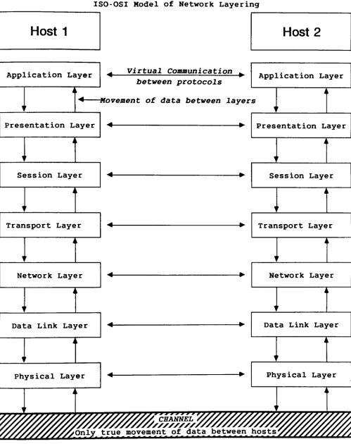
Under
the
7
Layered
OSI
model
[SHA
83]
(see
Figure
1)
there
exists
potential
for
a
queue-ing delay
at
every
layer.
Packets
may
have
to
wait
in
7
lines
to
have
physical,
data
link,
network,
transport,
session,
presenta
tion,
and
application
layer
services
performed
for
them.
Most
LANS
do
not
strictly
follow
the
OSI
approach;
however,
in
most
cases,
there
is
some
layering
involved
and
a
potential
for
FIGURE
1
ISO-OSI
Model
of
Network
Layering
Host
2
Application
Layer
^
Virtual
Communication
^
between
protocols
Application
Layer
<
Movement
of
data
between
layers
Presentation
Layer
Presentation
Layer
Session
Layer
Transport
Layer
Network
Layer
Data
Link
Layer
[image:16.543.16.515.39.669.2]In
order
to
measure
queueing
delays
between
layers,
timing
devices
are
needed
that
can
time
stamp
packets,
and
the
resolu
tion
of
the
devices
must
be
in
microseconds
[MUR
84].
What
is
of
interest
here
is
the
delay
incurred
when
a
packet
arrives
in
a
queue,
waits
for
service,
gets
serviced,
and
is
passed
onto
the
next
layer
for
service,
repeating
the
same
sequence
at
that
new
layer.
In
their
article
[MUR
84],
Murray
and
Enslow
point
out
several
specific
kinds
of
queuing
delay
experienced
in
an
ETHER
NET,
10Mbps,
Virtual
Circuit
LAN:
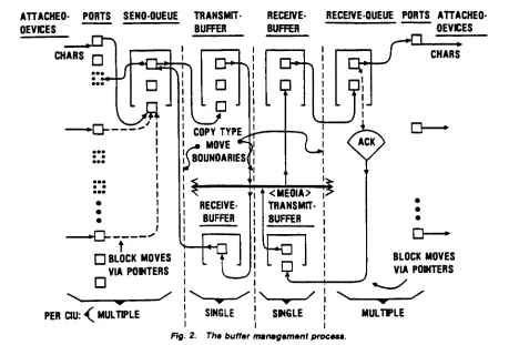
End-to-end
character
delivery
delays
are
simply
a
measure
of
how
long
it
takes
data
to
be
placed
into
a
packet,
transported
over
the
cable,
and
passed
onto
the
target
port
(Figure
2).
In
effect,
it
is
a
simple
view
of
the
birth
and
death
of
a
packet.
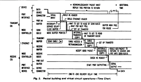
With
network
ports
operating
at
baud
rates
of
1200
bps
or
4800
bps
they
found
that
the
average
time
required
to
do
this
peaked
at
80ms
or
61ms
more
time
than
it
takes
to
send
a
single
asyn
chronous
character
over
a
leased
line
from
Boston
to
San
Fran-sisco!
See
Figure
3.
Murray
and
Enslow
broke
down
end-to-end
Figure
2.
(Adapted
from
[MUR
84])
Movement
of
packets
through
queues
and
buffers
endemic
to
virtual
circuit
protocols.
ATTACHED-
PORTS
SEND-QUEUE
TRANSMIT-
RECEIVE-DEVICES
BUFFER
BUFFER
RECEIVEOUEUE
PORTS
ATTACHED-DEVICES
JO^
CHARS
?
BLOCK MOVES
VIA POUTERS
?
y
CK^
D
COPY
TYPE
\s MOVE
^BOUNDARIES
K
RECEIVE
BUFFER
PER CIU:
<
MULTIPLE
t
<
MEDIA
>
TRANSMIT
BUFFER
SMGLE
y
CHARS
BLOCK MOVES
VIA
POMTERS
^r
[image:18.543.39.507.158.469.2]MULTPLE
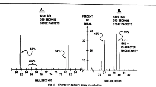
Figure
3.
(Adapted
from
[MUR
84])
Character
delivery
delay
distribution
showing
delay
peaks
at
61ms
and
81ms
for
network
ports
running
at
4800
and
1200
bps.
TRANSMIT,
QU
REEVE
cm
DEVICE
PORT
WTERFACE
WOE
CONTROUfR
ETHERNET
<WOE
CONTROUfR
PORT
HTERFACE
DEVICE
DATA
DEVICE
CONNECTOR
PORT-IN
BUFFER
SEND
QUEUE
TRANSMIT
BUFFER
RECSVE
BUFFER
RECSVE
QUEUE
PORT-OUT
BUFFER
DEVICE
CONNECTOR
~L
SERIAL
INPUT
INTERRUPT
SERVICE DELAY
CLOSE BUFFER
JlELAYl
L
*
ACKNOWLEDGEMENT PACKET MUST
REPEAT TUB PORTION
TO RETURN
. m
BUILD
VC HEADER
r
BUM ETHERNET
HEADER
-ADDITIONAL
TIME
rWAJT
TO
SET TO HEAO OF
SENO-QUEUE
r-WAITFOR NEXT POU
Cr
SET
UP
TRANSFER
BUFFER NOW
FREE
FOR
REUSE
MOVE BUFFER
POINTER*
(COAX
CABLE
()
INTERNAL
TRANSFER
(COPY)
r"'
[of
WATT
TRANSMIT-QUEUE
TO
GH
TD
HEAO
CABLE ACCESS*
RETRANSMISSION
H
CABLE
TRANSFER
(COPY)
ACCEPT SOOTJ PACKET
J TlSET UP TRANSFER
INTERNAL
TRANSFER
(COPY)
CHECK VC
HEADER
START
PORT
OUTPUTTING
-iI
I
IE
-IrBUILO
ACX-PACKET
TO
RETURN
TO
SENDER ANO
PUT INTO
SENO-QUEUE
SERIAL
OUTPUT
[image:19.543.33.505.157.433.2]'DATA
ENO-TD
-ENDDELIVERY DELAY TIME
Packet
building
and
buffer
management
delays
endemic
to
virtual
circuit
protocols
were
regarded
as
the
most
important
delays
in
the
study.
Performance
suffered
its
greatest
degrada
tion
in
these
two
activities.
Characters
that
need
to
be
transmitted
have
to
compete
for
a
limited
number
of
ports
and
buffers.
A
classic
queueing
delay
[KLE
64]
[KLE
70]
is
experi
enced
at
this
point
as
queueing
must
wait
for
ports
and
buffers
to
become
free
for
acquisition.
Once
a
buffer
is
acquired
for
data
another
queueing
delay
is
experienced
as
the
buffer
waits
to
move
to
the
head
of
the
send
queue
to
be
transmitted.
As
shown
in
Figure
4,
59%
of
the
80ms
end-to-end
delay
from
the
1200
bps
Figure
4.
(Adapted
from
[MUR
84])
Break
down
of
end
to
end
character
delivery
delays
\
+
52%
3.67.
A.
1200
b/s
300 SECONDS
35952
PACKETS
i
^
M
I
I
I
*
I
'l
h
PERCENT
OF
TOTAL
-40
40%
-n
30-
^*
10
-+
f-60
64
68
72
76
80
84
62
66
70
74
78
82
*VLAr
-20A
I-4800
b/s
300 SECONDS
37687 PACKETS
59%
(59%
y+i-0NE
-CHARACTER
UNCERTAINTY
[image:21.543.31.532.119.397.2]-I
I
1-77
79
81
76
78
80
82
MILLISECONDS
Fig. 5.
Two
serial
transfer
delays
contributed
significantly
to
the
80
ms
total.
An
8.3
ms
delay
was
attributed
to
the
movement
of
data
between
the
device
to
the
port
buffer
and
another
8.3
ms
delay
was
attributed
to
the
time
it
took
for
the
output
transfer.
These
and
other
delays
are
also
depicted
in
the
end-to-end
delivery delay
chart,
in
Figure
3.
2.1.1
Comments
It
should
be
noted
that
LANS
are
not
usually
used
to
package
and
send
1
character
at
a
time.
The
preceding
figures
may
be
a
little
misleading
if
it
causes
us
to
look
at
a
local
area
network
as
a
character-by-character
delivery
system.
The
fact
of
the
matter
is
that
LANS
deliver
massive
quantities
of
data
more
quickly
than
leased
lines.
Building
a
virtual
circuit
header
may
cost
no
more
time
for
a
packet
of
1500
bytes
than
for
a
hypothet
ical
packet
of
1
byte.
My
own
timing
tests
indicate
that
the
larger
the
file
being
moved
from
one
system
to
another,
the
fas
ter
the
transfer
rate.
This
indicates
that
the
overhead
involved
in
virtual
circuit
management
is
quickly
compensated
for
by
local
area
network
technology.
For
example,
transferring
a
281600
byte
file
from
one
system
to
another
over
a
10Mbps,
virtual
circuit
Ethernet
took
9.3
seconds.
This
was
a
transfer
rate
of
33
micro
seconds
per
character,
which
is
1000
times
faster
than
the
rate
reported
for
delivering
a
character
over
a
leased
line
from
Bos
transfer
a
1027
byte
file.
This
was
a
transfer
rate
of
1.2
mil
liseconds
to
deliver
1
character.
This
is
30
times
faster
than
the
leased-line
comparison
above.
In
short,
trying
to
compare
the
amount
of
data
that
can
be
transferred
by
a
LAN
verses
a
leased
line
in
the
same
amount
of
time
is
like
comparing
the
amount
of
water
that
moves
down
a
river
versus
a
garden
hose.
2.2
Analysis
of
Ethernet-like
Networks
[ALM
79]
The
discussion
of
delay
could
apply
to
Local
Area
Networks
of
varying
topologies
(
see
[CLA
76]).
This
chapter
will
discuss
network
metrics
that
specifically
apply
to
Ethernet-like
LANS,
[MET
76],
[ALM
79],
[MUR
84],
[
SHO
80].
The
network
that
is
con
sidered
in
this
sub-chapter
is
akin
to
the
original
Ethernet
explained
in
[MET
76].
That
is,
some
number
of
computers
have
time
division
multiple
access
to
a
broadcast
channel,
the
ether
(for
example,
a
coaxial
cable)
which
is
governed
by
a
distributed
control
policy.
Channel
time
can
be
divided
into
three
distinct
categories:
idle,
that
is
no
station
is
using
the
ether;
transmission,
that
is
one
station
has
seized
the
ether
and
is
sending
a
packet;
con-tention,
that
is
when
more
than
one
station
is
trying
to
transmit.
The
distributed
control
policy
is
the
means
by
which
sta-tion
is
ready
to
transmit
and
senses
an
idle
ether,
it
transmits.
Disregarding
random
errors,
(for
example,
checksum,
frame
errors,
etc)
in
the
time
it
takes
the
packet
to
traverse
the
channel
one
of
two
things
can
happen,
either
the
packet
will
arrive
safely
its
destination
or
it
will
suffer
a
collision.
Collisions
occur
when
one
or
more
stations
ready
to
transmit,
sense
an
idle
chan
nel
and
transmit
their
packets
simultaneously.
Collisions
also
occur
when
one
station
(A)
begins
transmitting
a
packet
while
at
least
one
other
ready
station
(B)
does
not
yet
sense
A's
packet
traveling
on
the
channel
due
to
signal
propagation
delay
and
transmits
thus
resulting
in
a
collision.
Signal
propagation
delay
is
the
amount
of
time
it
takes
for
a
signal
to
travel
from
one
point
to
another,
and
is
directly
proportional
to
the
dis
tance
between
them
(see
Figure
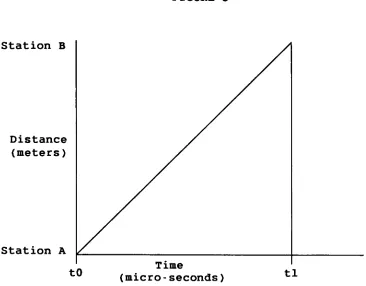
5).
Once
a
collision
is
sensed
by
the
stations
involved,
they
abort
transmitting
their
packets
and
FIGURE
5
Station
B
Distance
(meters)
Station
A
to
Time
(micro-
seconds
)
tl
Time
for
signal
to
propagate
between
stations
If
one
station
transmits
at
tO,
and
the
other
transmits
anytime
before
but
not
equal
to
tl,
there
[image:25.543.110.476.120.406.2]Contention
is
resolved
by
the
Binary
Exponential
Backoff
Algorithm
[MET
76]
given
below.
Ethernet
controllers
divide
retransmission
intervals
into
slots
which
represent
the
maximum
amount
of
time
between
starting
a
transmission
and
detecting
a
collision,
a
one
end-to-end
round
trip
delay.
An
Ethernet
con
troller
begins
transmission
of
each
new
packet
with
a
mean
retransmission
interval
of
one
slot
time.
Each
time
a
controller
detects
a
collision
it
attempts
retransmitting
the
packet
after
it
has
waited
a
random
interval
of
time
possessing
a
mean
twice
that
of
the
previous
interval,
plus
any
time
needed
to
wait
for
the
channel
to
clear
and
become
idle.
This
algorithm
tries
to
insure
that
as
a
contending
station
(one
of
two
or
more
stations
involved
in
a
collision)
becomes
ready
to
retransmit,
the
chance
of
doing
so
without
collision
is
increased
because
the
other
con
tending
stations
are
either
in
the
waiting
interval
or
have
already
attempted
retransmission.
As
stated
above,
in
analyzing
the
performance
of
an
Ether
net,
time
is
divided
into
slots
that
are
equal
to
the
round-trip
propagation
delay.
This
is
the
amount
of
time
that
it
takes
for
a
station
to
be
sure
that
its
signal
has
not
suffered
a
collision
from
the
most
distant
station.
The
instantaneous
load
(Q)
on
the
ether
is
considered
the
number
of
stations
that
desire
to
transmit
during
one
slot.
If
no
stations
transmit
(Q
=0),
the
slot
is
wasted
and
the
ether
is
idle.
If
Q
>
1
a
collision
occurs.
If
Q
=1,
one
station
seizes
the
ether
and
transmits
its
In
an
Ethernet
LAN
each
station
has
an
equal
chance
at
transmitting
whenever
the
channel
is
free.
There
is
no
forced
preference
or
priority
among
stations
at
any
time.
Metcalfe
and
Boggs
[MET
76]
describe
the
probability
that
one
station
acquires
the
ether
in
a
given
slot
as:
Q-l
A
=(1
-1/Q)
(1)
This
means
that
A
(acquisition
probability)
decreases,
as
Q
(the
number
of
stations
ready
to
transmit)
increases.
As
stated
above,
if
Q
is
greater
than
1
for
a
given
slot
there
will
be
a
collision
and
if
it
is
less
than
1,
no
station
seizes
the
either.
As
Q
increases,
out
to
infinity,
the
acquisition
probability
approaches
1/e
which
is
equal
to
1/2.7
(.
37)
or
a
37%
chance
that
the
ether
will
be
successfully
seized.
The
probability
that
the
ether
is
acquired
on
exactly
the
i-th
slot
is
i
A(l-A).
(2)
Equation
2
can
be
explained
by
the
following
simple
scenario.
Suppose
for
an
imaginary
network
of
2
computers
that
Q=2,
(both
stations
are
ready
to
transmit
at
the
same
time).
Both
stations
transmit
resulting
in
a
collision.
Both
stations
then
wait
a
random
amount
of
time
before
attempting
to
retransmit
(during
which
Q=0).
Due
to
this
waiting
period
more
slots
go
by
it
transmits
its
packet
without
a
collision
(e.g.
i=5),
provided
that
the
other
station
did
not
randomly
wait
the
same
amount
of
time,
then
the
other
station
becomes
ready
and
transmits
its
packet
(e.g.
i=9).
This
simple
scenario
demonstrates
that
if
there
are
2
or
more
stations
ready
to
transmit,
then
more
slots
available
to
them
(i
increasing)
results
in
a
higher
probability
that
they
will
acquire
the
channel.
In
other
words,
stations
may
not
acquire
the
first
few
"free"slots
that
go
by
due
to
colli
sion,
but
as
more
slots
go
by,
their
chances
of
acquisition
increases
with
each
slot.
Of
course,
the
scenarios
become
more
complex
as
the
number
of
hosts
involved
in
the
LAN
increases.
The
average
number
of
slots
devoted
to
contention
(eq.
3)
prior
to
acquiring
the
ether
is
expressed
by
the
following
equa
tion:
oo
1
Z
=SS
iA(l-A)
=(1-A)/A
(3)
i
=l
(Where
SS
=Sigma
and
oo
=infinity.)
Z
(the
average
number
of
slots)
increases
as
A
decreases
due
to
more
and
more
stations
that
desire
to
transmit
(an
increase
in
Q).
This
equation
leads
into
a
popular
LAN
metric:
channel
utiliza
2.3
Channel
Utilization
Almes
and
Lazowska
in
[ALM
79]
describe
channel
utilization
as
the
instantaneous
throughput
efficiency
of
the
network.
That
is,
the
ratio
of
the
proportion
of
time
the
network
is
success
fully
carrying
packets
(transmission
intervals)
to
the
proportion
of
time
the
network
is
busy
(transmission
intervals
plus
conten
tion
intervals)
when
the
instantaneous
load
Q
is
artificially
held
constant.
Instantaneous
throughput
efficiency
is
expressed
by
the
following
equation:
U
=(P/C)
(4)
(P/C)
+
2*tw*Z
where
P
is
the
average
packet
size
in
bits,
C
is
the
carrying
capacity
or
data
rate
of
the
ether
in
bits
per
second,
tw(greek:
tow)
is
the
propagation
delay
in
seconds,
multiplying
it
by
2
accounts
for
round-trip
propagation
delay,
which
is
the
slot
time,
and
Z
is
the
mean
number
of
slots
devoted
to
contention.
From
equation
4
it
can
be
seen
that
as
Z
increases
with
an
increase
in
instantaneous
load
(Q)
that
the
instantaneous
throughput
efficiency,
U
of
the
LAN
decreases.
Recall
that
Z
increases
as
A
decreases
with
a
rise
in
Q.
It
can
also
be
seen
that
as
average
packet
size
increases
that
U
will
increase.
Tw
can
increase
by
merely
lengthening
the
ether,
which
will
decrease
U.
As
C
increases
U
will
decrease
since
the
capacity
will
exceed
the
ability
of
the
LAN
stations
to
utilize
a
significant
portion
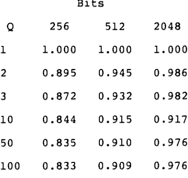
Table
1
displays
instantaneous
throughput
efficiency
for
various
instantaneous
loads
and
average
packet
sizes,
C
=3
Mbps,
2
x
tw
=10
usee.
Table
1
(Adapted
from
[ALM
79])
Instantaneous
throughput
efficiency
for
average
packet
sizes
of
256,
512,
and
2048
bits.
Cable
length
=1000m.
Data
rate
=3
Mbps.
Propagation
delay
=200
m/sec.
Bits
Q
256
512
2048
1
1.000
1.000
1.000
2
0.895
0.945
0.986
3
0.872
0.932
0.982
10
0.844
0.915
0.917
50
0.835
0.910
0.976
[image:30.543.176.369.250.432.2]The
adaptive
distributed
control
policy
designed
by
Metcalfe
and
Boggs
[MET
76]
is
inherently
stable.
This
stability
can
be
observed
by
calculating
the
asymptotic
instantaneous
throughput
efficiency
of
the
network.
From
equation
(1)
it
was
noted
that
as
Q
increases
A
approaches
1/e.
If
the
packet
size
is
held
to
the
minimum
size,
that
is
one
in
which
its
transmis
sion
time
equals
the
slot
time,
then:
1
11
0
= = = _(5)
1-A
1
+
(e
-1)
e
1
+
A
Put
in
simple
terms,
under
heavy
loads
the
throughput
of
the
net
work
will
be
at
least
1/e
times
the
network
carrying
capacity.
When
the
packet
size
is
increased
then
the
asymptotic
throughput
efficiency
should
be
much
larger
than
1/e.
[TAN
81]
takes
a
slightly
different
approach
to
calculating
instantaneous
throughput
efficiency
(utilization),
in
which
he
considers
an
ethernet
LAN
in
the
contention
state.
Recall
that
when
stations
are
in
contention
that
the
contention
resolution
algorithm
assigns
a
random
amount
of
time
that
a
station
must
wait
before
attempting
retransmission.
Therefore,
when
a
free.
slot
comes
up,
there
is
a
probability
(p)
that
the
station
will
transmit.
The
acquisition
probability,
A
(eq.
1)
becomes:
Q-l
A
=Qp(l
A
is
largest
when
p
equals
1/Q;
that
is
1
station
out
of
all
the
stations
in
contention
actually
gets
its
packet
out
onto
the
channel.
The
value
for
A
>l/e
as
Q
>oo.
Just
plug
some
big
numbers
for
Q
into
eq.
6
to
prove
this.
The
probability
that
the
contention
interval
has
exactly
j
slots
is:
j-l
A(l
-A)
eq.
7
So
the
mean
number
of
slots
per
contention
under
heavy
and
con
stant
loads
is:
oo
j-l
1
Z
=SS
jA(l
-A)
= =1
/(1/e)
=e
eq.
8
j=0
A
(S
=sigma
and
oo
=infinity)
Consequently,
the
previous
equation
for
utilization
(eq.
4),
mentioned
in
[ALM
79]
is
converted
to:
U
=P/C
eq.
9
P/C
+
2*tw*e
To
briefly
summarize
eq.
9,
in
dividing
time
into
slots,
each
slot
on
Ethernet
has
a
duration
of
2(round
trip)
*
tw,
and
that
the
mean
number
of
contention
slots
available
is
never
more
than
natural
'e',
(roughly
2.7).
Consequently
the
deterioration
in
utilization
due
to
propagation
delay
and
contention
for
Ethernet
is
never
more
than
2
x
e
x
tw
or
5.4tw,
even
under
heavy
and
con
stant
loads.
He
goes
on
to
report
that
tw
=5
microseconds
for
a
1
km
cable.
With
P
=1000
bits
utilization
U
=1000/lOMbps
-6
=1%
1000/lOMbps
-5.4
x
5
x
10
As
you
can
imagine,
LANS
that
have
channels
with
high
bandwidths
rarely
utilize
anywhere
near
100%
of
the
capacity-Stallings
in
[STA
84]
claims
that
the
two
most
useful
param
eters
in
analyzing
local
area
networks
are
the
data
rate
(C)
of
the
medium
and
the
average
signal
propagation
delay
(tw).
He
claims
that
the
product
of
Cx(tw)
is
the
most
important
factor
in
determining
the
performance
of
local
area
networks.
Under
ident
ical
conditions
a
50-Mbs,
1-km
bus
will
exhibit
the
same
utiliza
tion
as
a
10-Mbps,
5-km
bus.
The
article
points
out
that
the
product
of
Cx(tw)
is
equal
to
the
length
of
the
transmission
medium
in
bits,
that
is,
the
number
of
bits
physically
out
on
the
ether
and
traveling
between
two
nodes
at
a
given
instant.
Hence
both
of
the
networks
mentioned
have
the
same
bit
length,
50
bits.
[STA
84]
develops
yet
another
equation
for
channel
utiliza
tion
in
the
following
manner.
The
length
of
the
medium,
expressed
in
bits,
compared
to
the
average
packet
length
is
denoted
by
a:
Length
of
Data
Path
in
Bits
a
=Average
Packet
Length(P)
or
C
x
tw
/
P
a
=P/C
is
the
time
it
takes
to
get
the
average
packet
out
on
to
the
network.
So,
Propagation
Time
a
=Transmission
Time
Some
calculations
of
'a'for
Ethernet
LANS
of
different
lengths,
Table
2
(Adapted
from
[STA
84])
Values
of
'a'for
different
average
packet
sizes,
data
rates,
and
cable
lengths,
Data
Rate
Packet
Size
Cable
Length
a
1
Mbps
100
bits
1
km
0.05
1
Mbps
1000
bits
10
km
0.05
1
Mbps
100
bits
10
km
0.5
10
Mbps
100
bits
1
km
0.5
10
Mbps
1000
bits
1
km
0.05
10
Mbps
1000
bits
10
km
0.5
10
Mbps
10000
bits
1
km
0.05
50
Mbps
10000
bits
10
km
0.05
Utilization
is
defined
as
the
throughput
of
the
channel
divided
by
the
data
rate.
U
=number
of
bits
transmitted
number
of
bits
that
could
be
transmitted
U
=P/(
Propagation
+
Transmission
Time)
C
U
=P/(tw
+
P/C)
1
C
1
-a
When
the
number
of
slots
devoted
to
contention
and
round
trip
propagation
delay
is
factored
into
the
calculation:
U
=1
1
=
eq.
10
1
+
2aZ
1
+
(2*tw*Z)/(P/C)
So
far
three
different
equations
for
utilization
have
been
presented:
U
=P/C
/
(P/C
+
2*tw*Z)
eq.
4,
U
=P/C
/
(P/C
+
2*tw*e)
eq.
9,
U
=1
/
(1
+
(2*tw*Z)/(P/C)
)
eq.
10
In
fact,
they
are
all
different
forms
of
calculating
the
same
measurement
and
are
equivalent.
As
stated
in
its
presentation
with
different
values
of
Z
whereas
eq.
6
fixes
Z
at
e.
Infact
either
factor,
2*tw*Z
or
2*tw*e,
has
such
a
negligible
effect
on
the
final
outcome
of
the
calculation
for
utilization
that
it
really
does
not
matter
which
one
is
used;
with
Ethernets
running
at
10Mbps,
propagation
delay
is
so
small
(e.g.
2
microseconds)
that
multiplying
it
by
any
number
between
0
and
e
that
represents
the
mean
number
of
slots
spent
in
contention,
hardly
affects
the
final
value
of
U.
Given
the
10Mbps
LAN
exemplified
in
Chapter
2.3
the
reader
can
prove
this
to
himself
if
he
so
desires.
Equation
4
and
10
are
actually
different
forms
of
the
same
equation.
Equation
4
is
equation
10
with
P/C
factored
into
it
if
each
member
of
eq.
10
is
multiplied
by
P/C
it
is
transformed
into
eq.
4.
Both
will
result
in
the
same
value
for
U.
Contrary
to
the
opinion
in
[STA
84],
[TAN
81],
and
[SHO
80],
Almes
and
Lazowska
in
[ALM
79],
argue
that
utilization
is
not
a
very
meaningful
performance
measurement
because
Q,
the
number
of
stations
ready
to
transmit,
must
be
held
artificially
constant.
They
prefer
to
base
other,
more
meaningful
metrics
on
the
average
load
,Ro
,experienced
by
the
network.
Average
load
is
defined
in
[TAN
81]
as
the
ratio
of
packets
entering
the
network
to
the
number
of
packets
leaving
the
network
during
a
given
time
period.
In
other
words,
it
is
the
ratio
of
arrival
rate
of
packets
into
the
network
to
the
mean
service
rate
of
the
network
hosts.
The
mean
service
rate
is
equal
to
1
packet
length
P,
stations
submit
packets
onto
the
ether
at
an
average
rate
of
Ro*C/P
per
second.
Almes
and
Lawozowska
use
these
values
to
determine
the
following
metrics:
o
the
proportion
of
capacity
used
to
resolve
contention
times,
o
Throughput
efficiency
of
the
network.
That
is
the
ratio
of
the
proportion
of
time
the
network
is
successfully
carrying
packets
to
the
proportion
of
time
the
network
is
transmitting
and
con
tending.
o
Average
response
time
of
the
network.
That
is,
the
average
amount
of
time
it
takes
for
a
station
to
successfully
transmit
a
packet,
after
the
point
at
which
it
was
ready
to
transmit
it.
Note:
I
think
that
this
is
a
poor
definition
for
this
metric.
Almes
and
Lazowska
look
at
this
metric
as
if
the
ether
"responds"to
a
stations
desire
to
send
a
packet
and
that
the
amount
of
time
a
station
has
to
wait
around
is
the
measure
of
the
response
time
of
the
ether.
It
seems
that
this
metric
should
be
called
average
WAITING
time,
instead.
This
will
become
even
clearer
in
the
fol
lowing
equations.
o
Perceived
efficiency
of
the
network.
That
is,
the
ratio
of
the
theoretical
transmission
time
for
a
packet
of
length
P
to
the
average
response
time
seen
by
a
station
transmitting
packets
of
that
size.
In
[ALM
79]
an
Ethernet
simulation,
using
a
Markov
model,
transmission,
contention,
and
idle
states
for
varying
average
loads
for
packets
of
256
and
2048
bits,
and
for
a
carrying
capa
city
of
3
Mbps.
The
results
are
shown
in
Figure
6.
As
the
aver
age
number
of
packets
submitted
onto
the
network
over
time
increases,
the
number
of
transmissions
increases
proportionally
until
the
asymptotic
throughput
efficiency
(Eq.
5)
is
reached
for
that
packet
size.
Beyond
this
point,
the
network
enters
the
con
tention
state.
In
other
words,
Figure
6
shows
that
as
packets
are
infrequently
submitted
onto
the
channel
(i.e.
small
average
load
per
small
proportion
of
time)
that
few
collisions
occur
and
that
most
transmissions
succeed.
As
the
number
of
transmissions
increases,
so
does
the
offered
load
and
the
number
of
collisions,
thereby
resulting
in
more
stations
spending
time
in
contention
resolution.
Notice
that
the
graph
with
the
smaller
packet
size
spends
more
time
in
contention
resolution.
This
is
due
to
the
fact
that
with
shorter
packets
there
is
a
shorter
transmission
Figure
6.
(Adapted
from
[ALM
79])
Ethernet
time
divided
into
idle,
contention
and
transmission
time
1.01
-1.0
0.0*^
0.0
average
load
; averageicac
cFigure
2-1:
Time
Tranci
1 1 ir.f
,Contending,
Idie
[image:40.543.77.469.180.354.2]The
simulation
also
produced
results
for
average
response
times,
as
shown
in
Figure
7.
As
average
load
increases
the
response
time
slowly
increases,
until
the
average
load
reaches
the
asymptotic
throughput
efficiency.
Then
a
sharp
increase
in
response
time
is
manifested,
as
shown
by
the
knee
in
the
curve.
Here
the
larger
packet
size
is
more
detrimental
to
this
perfor
Figure
7.
(Adapted
from
[ALM
79])
Average
load
vs.
average
response
time.
5
..1)
256
0.0
average
load
p
1.0
5
,CO
average
load
p
1.0
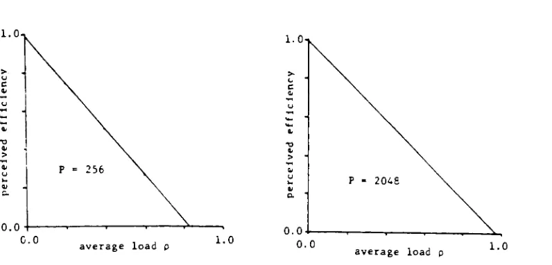
[image:42.543.90.452.152.324.2]The
simulation
also
produced
results
for
perceived
effi
ciency;
that
is,
the
ratio
of
theoretical
packet
transmission
time
to
average
response
time
for
packets
of
average
length
P.
As
shown
in
Figure
8,
perceived
efficiency
decreases
linearly
with
increased
average
load
and
reaches
zero
for
an
average
load
equal
to
the
asymptotic
throughput
efficiency.
At
this
point,
stations
are
attempting
to
send
packets
faster
than
the
network's
ability
to
carry
them
and
most
of
the
time
is
spent
in
contention
1.0,
0.0
Figure
8.
(Adapted
from
[ALM
79])
Perceived
efficiency
vs.
average
load.
CO
average
load
p
1.0
1.0
0.0
0.0
average
load
p
1.0
[image:44.543.89.487.128.319.2]Relative
load
is
defined
as
the
ratio
of
the
average
load,
Ro,
to
the
asymptotic
throughput
efficiency,
for
a
packet
of
average
size,
P.
Almes
and
Lazowska
observed
that
for
a
specific
relative
load,
that
perceived
efficiency
is
equal
to
1
-(relative
load).
This
makes
perceived
efficiency
much
easier
to
measure
and
calcu
late.
Other
calculations
become
simpler
through
this
observation.
For
example,
given
a
network
with
an
observed
average
packet
size
of
P,
an
observed
average
load
of
Ro,
and
and
asymptotic
throughput
efficiency
of
U,
the
relative
load
is
RL
=Ro
/
U
(11)
and
the
perceived
efficiency,
is
PE
=1
-RL.
(12)
Linking
this
new
definition
of
perceived
efficiency