Camera Motion Estimation for Multi-Camera Systems

(1)

Camera Motion Estimation for

Multi-Camera Systems

Jae-Hak Kim

A thesis submitted for the degree of Doctor of Philosophy of The Australian National University

(2)

This thesis is submitted to the Department of Information Engineering, Research School of Information Sciences and Engineering, The Australian National University, in fullfilment of the requirements for the degree of Doctor of Philosophy.

This thesis is entirely my own work, except where otherwise stated, describes my own research. It contains no material previously published or written by another person nor material which to a substantial extent has been accepted for the award of any other degree or diploma of the university or other institute of higher learning.

Jae-Hak Kim 31 July 2008 Supervisory Panel:

Prof. Richard Hartley Dr. Hongdong Li Prof. Marc Pollefeys Dr. Shyjan Mahamud

The Australian National University The Australian National University ETH, Z¨urich National ICT Australia In summary, this thesis is based on materials from the following papers, and my per-cived contributions to the relevant chpaters of my thesis are stated:

Jae-Hak Kim and Richard Hartley, “Translation Estimation from Omnidirectional Images,” Digital Im-age Computing: Technqiues and Applications, 2005. DICTA 2005. Proceedings, vol., no., pp. 148-153, Dec 2005, (80 per cent of my contribution and related to chapter 6)

Brian Clipp, Jae-Hak Kim, Jan-Michael Frahm, Marc Pollefeys and Richard Hartley, “Robust 6DOF Motion Estimation for Non-Overlapping, Multi-Camera Systems,” Applications of Computer Vision, 2008. WACV 2008. IEEE Workshop on , vol., no., pp.1-8, 7-9 Jan 2008, (40 per cent of my contribu-tion and related to chapter 7)

Jae-Hak Kim, Richard Hartley, Jan-Michael and Marc Pollefeys, “Visual Odometry for Non-overlapping Views Using Second-Order Cone Programming,” Asian Conference on Computer Vision, Tokyo, Japan, ACCV (2) 2007, pp. 353-362 (also published in Lecture Notes in Computer Sciences, Springer, Volume 4844, 2007), (80 per cent of my contribution and related to chapter 8)

Hongdong Li, Richard Hartley, and Jae-Hak Kim, “Linear Approach to Motion Estimation using a Generalized Camera,” IEEE Computer Society Conference on Computer Vision and Pattern Recogni-tion (CVPR 2008), Anchorage, Alaska, USA, 2008, (30 per cent of my contribuRecogni-tion and related to chapter 9)

Jae-Hak Kim, Hongdong Li and Richard Hartley, “Motion Estimation for Multi-Camera Systems using Global Optimization,” IEEE Computer Society Conference on Computer Vision and Pattern Recogni-tion (CVPR 2008), Anchorage, Alaska, USA, 2008, (80 per cent of my contribuRecogni-tion and related to chapter 10)

Jae-Hak Kim, Hongdong Li and Richard Hartley, “Motion Estimation for Non-overlapping Multi-Camera Rigs: Linear Algebraic and L∞ Geometric Solutions,” submitted to IEEE Transactions on Pattern Analysis and Machine Intelligence, 2008, (70 per cent of my contribution and related to chapters 9 and 10)

(3)

(4)

(5)

Acknowledgements

I would like to sincerely thank Prof. Richard Hartley for giving me the opportunity to study at the Australian National University and at NICTA and for supervising me during my Ph.D.

course. His guidance gave me a deep understanding of multiple view geometry and truly let

me know how beautiful geometry is. I would like to thank Dr. Hongdong Li, who gave me a lot of advice on my research work and encouraged me to conceive new ideas. I would

also like to thank Prof. Marc Pollefeys, who gave me a chance to visit his vision group at

the University of North Carolina, Chapel Hill, as a visiting student and inspired me to find a research topic for my Ph.D. thesis. I also thank Dr. Shyjan Mahamud, who directed my

approach to solving problems. I would like to thank National ICT Australia (NICTA) for providing Ph.D. scholarships during the last four years.

I would like to thank Dr. Jan-Michael Frahm for many discussions about this research as

well as other members of the vision group at the UNC-Chapel Hill – Dr. Jean-Sebastien Franco, Dr. Philippos Mordohai, Brian Clipp, David Gallup, Sudipta Sinha, Paul Merrel, Changchang

Wu, Li Guan and Seon-Ju Kim. They gave me a warm welcome and provided good research

atmosphere during my visit to UNC-Chapel Hill.

I would like to thank Prof. Berthold K. P. Horn and Prof. Steve Maybank who answered

my questions and discussed the history and terminologies of epipolar geometry via emails. I

would also like to thank Dr. Jun-Sik Kim who pointed out an error in a figure that has been used in this thesis.

I also thank Prof. Joon H. Han, Prof. Daijin Kim, Prof. Seungyong Lee, Prof. Yongduek

Seo and Prof. Jong-Seung Park. They have been my strongest support from Korea, and they have shown me how exciting and interesting computer vision is.

I would also like to thank people and organizations for providing me pictures and

illus-trations that are used in my thesis – AAAS, AIST, Breezesystems Inc., Dr. Carsten Rother, Google, The M.C. Escher Company, NASA/JPL-Caltech, Point Grey Research Inc., Prof.

Richard Hartley, Sanghee Seo, Dr. Simon Baker, Timothy Crabtree, UNC-Chapel Hill and

Wikipedia.

I am grateful to the RSISE graduate students and academic staff – Andreas M. Maniotis,

Dr. Antonio Robles-Kelly, Dr. Arvin Dehghani, Dr. Brad Yu, Dr. Chanop Silpa-Anan, Dr.

Chunhua Shen, Desmond Chick, Fangfang Lu, Dr. Guohua Zhang, Dr. Hendra Nurdin, Jae Yong Chung, Dr. Jochen Trumpf, Junae Kim, Dr. Kaiyang Yang, Dr. Kristy Sim, Dr. Lei

Wang, Luping Zhou, Manfed Doudar, Dr. Nick Barnes, Dr. Paulette Lieby, Dr. Pei Yean Lee,

(6)

Pengdong Xiao, Peter Carr, Ramtin Shams, Dr. Robby Tan, Dr. Roland Goecke, Sung Han

Cha, Surya Prakash, Tamir Yedidya, Teddy Rusmin, Vish Swaminathan, Dr. Wynita Griggs, Yifan Lu, Yuhang Zhang and Zhouyu Fu. They welcomed me to RSISE and helped me survive

as a Ph.D. student in Australia.

I would also like to thank Hossein Fallahi and Dr. Andy Choi, who were residents with me at Toad Hall.

I would like to thank my close friends from Korea – Jongseung Kim, Jaenam Kim,

Hui-jeong Kim, Yechan Ju, Hochan Lim, Kyungho Kim and Jaewon Jang – who supported me. I also thank my friends in POSTECH – Hyukmin Kwon, Semoon Kil, Byunghwa Lee,

Jiwoon Hwang, Dr. Kyoo Kim, Yumi Kim, Dr. Hyeran Kim, Hyosin Kim, Dr. Sunghyun Go,

Dr. Changhoon Back, Minseok Song, Dr. Hongjoon Yeo, Dr. Jinmong Won, Dr. Gilje Lee, Sookjin Lee, Hyekyung Lim, Chanjin Jeong and Chunkyu Hwang.

I would like to thank the Korean students in Canberra – Anna Jo, Christina Yoon, Eunhye

Park, Eunkyung Park, Haksoo Kim, Inho Shin, Jane Hyo Jin Lee, Kyungmin Lee, Mikyung Moon, Miseon Moon, Sanghoon Lee, Sangwoo Ha, Se-Heon Oh, Sung-Hun Lee, Taehyun

Kim, Thomas Han and Wonkeun Chang. They have been so kind to me as the same

interna-tional student studying in Australia. I will never forget the good times that we had together. In particular, I would like to thank Fr. Albert Se-jin Kwon, Fr. Michael Young-Hoon Kim,

Br. Damaso Young-Keun Chun and Fr. Laurie Foote. for provding spiritual guidance.

Last, but not the least, I would like to thank my relatives and familiy – Clare Kang, Gloria Kim, Natalie Kim, Yunmi Kim, Hyuncheol Kim, Hocheol Kim, Yeonmi Kim, my father and

my mother. I would especially like to thank my wife, Eun Young Kim, who supported me with

her love and sincere belief. Also, thank my little child to be borned soon.

(7)

Abstract

The estimation of motion of multi-camera systems is one of the most important tasks in

com-puter vision research. Recently, some issues have been raised about general camera models

and multi-camera systems. Using many cameras as a single camera is studied [60], and the

epipolar geometry constraints of general camera models is theoretically derived. Methods for

calibration, including a self-calibration method for general camera models, are studied [78, 62].

Multi-camera systems are an example of practically implementable general camera models and

they are widely used in many applications nowadays because of both the low cost of digital

charge-coupled device (CCD) cameras and the high resolution of multiple images from the

wide field of views. To our knowledge, no research has been conducted on the relative

mo-tion of multi-camera systems with non-overlapping views to obtain a geometrically optimal

solution.

In this thesis, we solve the camera motion problem for multi-camera systems by using

lin-ear methods and convex optimization techniques, and we make five substantial and original

contributions to the field of computer vision. First, we focus on the problem of translational

motion of omnidirectional cameras, which are multi-camera systems, and present a constrained

minimization method to obtain robust estimation results. Given known rotation, we show that

bilinear and trilinear relations can be used to build a system of linear equations, and singular

value decomposition (SVD) is used to solve the equations. Second, we present a linear method

that estimates the relative motion of generalized cameras, in particular, in the case of

non-overlapping views. We also present four types of generalized cameras, which can be solvable

using our proposed, modified SVD method. This is the first study finding linear relations for

certain types of generalized cameras and performing experiments using our proposed linear

method. Third, we present a linear 6-point method (5 points from the same camera and 1 point

from another camera) that estimates the relative motion of multi-camera systems, where

(8)

vii

eras have no overlapping views. In addition, we discuss the theoretical and geometric analyses

of multi-camera systems as well as certain critical configurations where the scale of translation

cannot be determined. Fourth, we develop a global solution under anL∞ norm error for the relative motion problem of multi-camera systems using second-order cone programming.

Fi-nally, we present a fast searching method to obtain a global solution under anL∞norm error for the relative motion problem of multi-camera systems, with non-overlapping views, using a

branch-and-bound algorithm and linear programming (LP). By testing the feasibility of LP at

the earlier stage, we reduced the time of computation of solving LP.

We tested our proposed methods by performing experiments with synthetic and real data.

The Ladybug2 camera, for example, was used in the experiment on estimation of the translation

of omnidirectional cameras and in the estimation of the relative motion of non-overlapping

(9)

Introduction

In this thesis, we investigate the relative motion estimation problem of multi-camera systems to

develop linear methods and a global solution. Multi-camera systems have many benefits such

as rigid motion for all six degrees of freedom without 3D reconstruction of the scene points.

Implementations of multi-camera systems can be found in many applications but few studies

have been done on the motion of multi-camera systems so far.

In this chapter, we give a general introduction to multi-camera systems and their

applica-tions, followed by our contributions and an overview of this thesis.

Recently, the popularity of digital cameras such as digital SLR (single-lens reflex) cameras,

compact cameras and mobile phones with built in camera has increased due to their decreased

cost. Barry Hendy from Kodak Australia [29] plotted the “pixels per dollar” as a basic measure

of the value of a digital camera and used the information to recommend a retail price for Kodak

digital cameras. This law is referred to as “Hendy’s Law”. On the basis of this law, it can be

concluded that the resolution of a digital camera is becoming higher and the price per pixel of

the camera sensor is becoming lower every year. It is no longer difficult or expensive to set up

an application that uses several cameras.

It is considered that multicamera systems (a cluster of cameras or a network of cameras)

have many benefits in real applications such as visual effects and scientific research. The first

study on virtualized reality projects that use virtual views captured by a network of cameras

was conducted by Kanade et al. in 1995 [54]. Their system was used to capture touchdowns

in the Super Bowl, which is the championship game of professional American football, and it

was used to look around the event from other point of virtual views. In 1999, a similar visual

(15)

2

Figure 1.1: A software controlling 120 cameras using 5 laptops.www.breezesys.com(Courtesy of Breezesystems, Inc)

effect known as “bullet time” was implemented in the film “The Matrix”, where the camera

appears to orbit around the subject of the scene. This was done by placing a large number of

cameras around the subject of the scene. Digital Air is a well-known company that produces

Matrix-like visual effects for commercial advertisements [9]. Another company, Breezesys,

Inc. [6], sells consumer-level software that allows the simultaneous capture of multiple images

by multiple cameras controlled by a single laptop, as shown in Figure 1.1. Thus, the use of

multi-camera systems in various applications is becoming popular and their use is expected to

increase in the near future.

In the last two decades, many studies have been conducted on the theory and geometry

of single-camera systems which are used to capture images from two views, three views and

multiple views [11, 10, 27]. However, the theory and geometry of multi-camera systems have

not been fully studied or clarified yet. This is because in addition to recording multiple views

of a scene using a network of cameras or an array of cameras, there are more challenging tasks

such as obtaining spatial and temporal information as the multi-camera system moves around

the environment.

This process of obtaining the orientation and position information is known as the “visual

odometry” problem or “the problem of estimation of relative motion of multi-camera systems”.

(16)

[image:16.612.118.524.111.428.2]

3

Figure 1.2: The Mars Exploration Rovers in motion. The rovers are equipped with 9 cameras: four

Hazcams are mounted on the front and rear ends for hazard avoidance, two Navcams are mounted on the head of the rovers for navigation, two Pancams are mounted on the head to capture panoramas, and one micoscopic camera is mounted on the robotic arm. (Courtesy NASA/JPL-Caltech)

landed on Mars in January 2004. As shown in Figure 1.2, these rovers were equipped with nine

cameras distributed between their heads, legs and arms. Although the rovers were equipped

with navigation sensors such as IMU (inertial measurement unit) and odometry sensors on

their wheels, the estimated distance travelled by the rovers on Mars was not very accurate.

This could have been due to several reasons, for example, the rover wheels could not obtain

a proper grip on the ground on Mars, which caused the wheels to spin without moving. This

resulted in the recording of false measurements by the odometry unit. Another reason could

have been the accidental failure of the IMU and odometry equipment. In such a case, visual

sensors such as the nine cameras might be used to determine the location of the rovers on Mars.

(17)

§1.1 Problem definition 4

motion of multi-camera systems. Hence, if we develop an optimal solution, it can be applied to

control the motion of planetary rovers, UAVs (unmanned aerial vehicles), AUVs (autonomous

underwater vehicles) and domestic robots such as Spirit and Opportunity on Mars, Aerosonde,

REMUS and iRobot’s Roomba.

In general, the motions of camera systems can be considered to be Euclidean motions that

have six degrees of freedom in three-dimensional (3D) space. So, the main aim of this study

is to estimate the motion for all six degrees of freedom. However, in single-camera systems

that capture two images, the relative motion can be estimated for only five degrees of freedom:

three degrees for rotation and two degrees for translation direction. The scale of translation

cannot be estimated from the single-camera system unless 3D structure is recovered. However,

in the case of non-overlapping multiple rigs, 3D structure recovery problem is not as easy as

in the case of systems with overlapping views such as stereo systems and monocular SLAM

(Simultaneous Localization and Mapping) systems.

1.1 Problem definition

In this thesis, we investigate the motion of multi-camera systems. We investigate motion

es-timation problems such as the translational motion of an omni-directional camera, the motion

of a non-overlapping 8-camera system on a vehicle using a linear method and the motion of a

6-camera system (Ladybug2 camera) using second-order cone programming (SOCP) or linear

programming (LP) underL∞norm.

In general, the motion of multi-camera systems is a rigid motion. Therefore, there are 6

degrees of freedom for rotation and translation. Taking advantage of the spatial information

(exterior calibration parameters) of cameras in multi-camera systems, we can estimate the

relative motion of multi-camera systems for six degrees of freedom.

Given known camera parameters, we capture image sequences using a multi-camera

sys-tem. Then, pairs of matching points are detected and found using feature trackers. Using these

pairs of matching points, we estimate the relative motion of multi-camera systems for all the

(18)

§1.2 Contributions 5

1.2 Contributions

In this thesis,

1. We show that if the rotation of the camera across multiple views is known, it is possible

to estimate the translation more accurately using a constrained minimization method

based on singular value decomposition (SVD).

2. We also show that the motion of non-overlapping images can be estimated from a

min-imal set of 6 points of which 5 points are from one camera and 1 point is from another

camera. Theoretical analysis of the critical configuration that makes it impossible to

solve the relative motion of multi-camera systems is also studied.

3. A linear method to estimate the orientation and position of a multi-camera system (or

a general camera model) is studied by considering the rank deficiency of equations and

experiments. To our knowledge, no experiments using linear methods have been

per-formed by other researchers in the field of computer vision.

4. Using global optimization and the convex optimization techniques, we solved the

prob-lem of estimation of motion using SOCP.

5. We solved the problem of estimation of motion using LP with a branch-and-bound

algo-rithm. Approaches 4 and 5 provide a framework to obtain a global solution for the

prob-lem of estimation of relative motion in multi-camera systems (even with non-overlapping

views) under theL∞norm.

We performed experiments with synthetic and real data to verify our algorithms, and they

mostly showed robust and good results.

1.3 Overview

In chapter 1, we provide a general overview of the problems in the estimation of multi-camera

(19)

§1.3 Overview 6

In chapters 2 to 4, we provide brief overviews of the single-camera system, two-camera

system, three-camera system, multi-camera system and their motion estimation problems. In

chapter 5, we discuss previous related works.

The main work of this thesis is presented in chapters 6, 7, 8, 9 and 10. In chapter 6, we

show how constrained minimization allows the robust estimation from omnidirectional

im-ages. In chapter 7, we show how using six points, we can estimate the relative motion of

non-overlapping views, and we also show that there is a degeneracy configuration that makes

it impossible to estimate the motion of non-overlapping multi-camera rigs. In chapter 8, we

re-veal a linear method for estimation of the motion of a general camera model or non-overlapping

multi-camera systems along with an intensive analysis of the rank deficiency in generalized

epipolar constraint equations. In chapter 9, we study the geometry of multi-camera systems

and demonstrate how using their geometry, we can convert the motion problem to a convex

optimization problem using SOCP. In chapter 10, we attempt to improve the method proposed

in chapter 9 by developing a unified framework to derive a global solution for the problem

of estimation of camera motion in multi-camera systems using LP and a branch-and-bound

(20)

Chapter 2

Single-Camera Systems

2.1 Geometry of cameras

In this section, we revisit the geometry of single-camera systems and present a detailed analysis

of the projection of points in space onto an image plane and the rigid transformations of points

and cameras.

Let us assume that the world can be represented using a projective spaceIP3. The structures

and shapes of objects are represented using points in the form of 4-vectors such asXinIP3_.

The motion of these points is represented by a3_×3rotation matrixR_{and a 3-vector translation}

t. Let us now consider transformations of points and cameras in the projective spaceIP3_.

Three coordinate systems are used to describe the positions of points, the locations of

cameras in the projective space IP3 and the image coordinates inIP2. In this study, we have

used right-hand coordinate systems, as shown in Figure 2.1. The first coordinate system is

the world coordinate system, which is used to represent the positions of points and cameras in

y

x

z

=

x

_×

y

Figure 2.1: Right-hand coordinate system.

(21)

§2.1 Geometry of cameras 8

Xcamera

Zcamera

Ycamera

Zworld

Xworld

Yworld

(a) Camera and scene structure in the world coordinate system

Yimage

Ximage

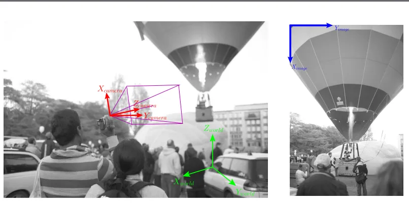
[image:21.612.117.520.92.292.2]

(b) Projected image

Figure 2.2: (a) The camera coordinate system (indicated in red) is represented by the basis vectors Xcamera,YcameraandZcamera, and the world coordinate system (indicated in green) is represented by the basis vectors Xworld, Yworld andZworld in 3D space. (b) The image coordinate system is represented by two vectorsXimageandYimagein 2D space.

the world. Hence, the positions of all points and cameras can be represented by an identical

measurement unit such as “metre”. The second system is the camera coordinate system, in

which the positions of the points are based on the viewpoints of the cameras inIP3. It should

be noted that a point in space can be expressed both in the world coordinate system and in the

camera coordinate system. The final coordinate system is the image coordinate system, which

is specifically used to define the coordinates of pixels in images. Unlike the first two coordinate

systems, the image coordinate system is inIP2_{. The image coordinate system uses “pixels” as}

the unit of measurement.

Figure 2.2 shows the three coordinate systems. In Figure 2.2(a), we observe that the person

holding the camera is taking a picture of a balloon. A camera has its own two-dimensional

(2D) coordinate system for images. This 2D coordinate system is shown in Figure 2.2(b). The

camera is positioned with respect to a reference point in the world coordinate system. The

position of the balloon in the air can also be defined with respect to the reference point in

the world coordinate system. Therefore, the positions of the camera and balloon (structure)

(22)

coordinate system (indicated in red) is positioned at the centre of the camera and points toward

the object of interest.

2.1.1 Projection of points by a camera

If we assume that thez-axis of the camera is aligned with thez-axis of the world coordinate

system, and the two coordinate systems are placed at the origin, then the camera projection

matrix can be represented by a3_×4matrix as follows:

P_{= [}I_|₀_] _(2.1)

whereI_{is a}₃_×₃_{identity matrix.}

Let a 4-vectorXcambe a point in space andXcambe represented in the camera coordinate

system. Then,Xcammay be projected onto the image plane of the camera through a lens. The

image plane uses a 2D image coordinate system, as shown in Figure 2.2(b). Therefore, the

projected pointxis represented as a 3-vector inIP2and can be denoted as follows:

x= [I_|₀_]_X_cam _(2.2)

It should be noted thatxstill uses the same unit (say “metre”) as that of the world

coordi-nate system in (2.2). However, as we are dealing with images, this unit needs to be converted

to a pixel unit. Most digital cameras have a charge-coupled device (CCD) image sensor that

is only a few millimetres in size. For instance, the Sony ICX204AK1is a6-mm(= 0.24in)

diagonal, interline CCD solid-state image sensor with a square pixel array, and it has total of

1024_×768active pixels. The unit cell size of each pixel is4.65µm_×4.65µm2_{. Therefore,} the units needed to be converted in order to obtain the coordinates of a pixel in the image. For

instance, in Sony ICX204AK CCD sensors, the size of a pixel is4.65_×10−₆

metres. Hence,

this value is multiplied by1/(4.65_×10−₆

)in order to convert the unit from metres to pixels.

It is also necessary to consider other parameteres such as the focal length, the principal

1_{Sony ICX204AK technical document [33]}

2₁

(23)

points where the optical axis meets the image plane, and the skewness of the image sensor. All

these parameters are included in a3_×3matrix, which is termed a “calibration matrix”. The

calibration matrix may be added in (2.2) and it is given as follows:

x=K_[I_|₀_]_X_cam _(2.3)

whereK_{has focal lengths}_f_x_and_f_{y, and the skew parameter}_s_{, and it is defined as}

K₌



    

fx s 0

0 fy 0

0 0 1



    

. (2.4)

The units of the focal lengthsfxandfyshould be converted from metres, the unit of the world

coordinate system, to pixels, the measurement unit of images.

2.1.2 Rigid transformation of points

A rigid transformationM_{of a point}_X_in_IP3_{is given as follows:}

X′ =M_X_, _(2.5)

whereM_{is a}₄_×₄_{matrix used for transformation and}_X′_{is the position of}_X_after transforma-tion ofX. This transformation may be considered to represent the pointXafter rotation and

translation. Thus, (2.5) may be rewritten as follows:

X′=



 

R ₋R_t

0⊤ 1





X, (2.6)

whereR_{is a}₃_×₃_{rotation matrix and}_t_{is a 3-vector translation. Please note that the point}_X

is translated bytfirst and then rotated byR_{with respect to the world coordinate system. This}

(24)

y

X

′

X

R

,

t

x

z

Figure 2.3: Rigid transformation of a point. A pointXis moved to a different positionX′by a rigid motion comprising rotationR_{and translation}_t_.

2.1.3 Rigid transformation of cameras.

Let us now consider the rigid transformation of the coordinates of a camera, as shown in

Fig-ure 2.4. The camera is placed in the world coordinate system, so its coordinate transformation

has rotation and translation parameters similar to the transformation of points.

A camera aligned with the axis of the world coordinate system at the origin is represented

by a3_×4matrix as follows:

P_{= [}I_|₀_]_, _(2.7)

whereI_{is a}₃_×₃_{identity matrix.}

If the camera is positioned at a pointc, the camera matrix is represented as follows:

P₌



    

1 0 0 ₋cx

0 1 0 ₋cy

0 0 1 ₋cz



    

, (2.8)

where the vectorc= [cx, cy, cz] ⊤

is the centre of the camera. The left3_×3submatrix inP_is

not changed because the camera is still aligned with the world coordinate system.

(25)

c

X

y z x

x′

y′ z′

R_, _t

c′

Figure 2.4: Rigid transformation of a camera. A camera atcis moved to a positionc′ by a rigid motion comprising rotationR_{and translation}_t_.

positioned camera matrix can be represented as follows:

P₌R_[I_{| −}_c_{] = [}R_{| −}R_c_{] = [}R_|_t_]_, _(2.9)

wheret=₋R_c_{is a vector represented by the translation}3_.

In particular, note that the camera is first translated by t and is then rotated by R _with

respect to the world coordinate system. Finally, the camera is positioned atc. A pointXin

IP3is projected onto an image pointvinIP2by the camera matrixP_{as follows:}

v=P_X₌R_[I_{| −}_c_]_X_, _(2.10)

where v is a 3-vector in IP2 and is represented in the image coordinates. Hence, v can be

considered as an image vector originating from the centre of the camera to the pointX. IfX

is displaced by the motion matrixM_{, then the projection of}_X_{is also displaced as follows:}

v′ =PM_X₌R_[I_{| −}_c_]M_X_. _(2.11)

3_{The vector}_t_{is also called a translation in other articles. However, probably it is more reasonable to define}_c_as

a translation instead oft_{because it is more relevant to our geometrical concepts. For better understanding, in this}

(26)

§2.2 Epipolar geometry of two views 13

Instead of moving X, let us imagine that the camera is moved to make the position of the

projected point the same as that ofv′. Therefore, from (2.11), the matrixP′_{of the transformed} camera matrix is written as:

P′ ₌PM₌R_[I_{| −}_c_]M_. _(2.12)

Let us consider two rigid transformations M₁ _and M₂_{. Let the transformations be applied}

in the orderM₁ _andM₂ _{to a point} _X_{. The transformed point is denoted as} _X′ ₌ M₂M₁_X_{. In} the same way, the transformed camera matrix can be given byP′ ₌PM₂M₁ _{instead of moving} points.

2.2 Epipolar geometry of two views

In this section, we revisit the geometry of single-camera systems used to capture two images

from two different locations and also re-introduce methods to estimate the relative motion of

a camera between two views. In the following section, we distinguish between two terms

“views” and “cameras” in order to better understand multi-camera systems.

2.2.1 Definitions of views and cameras

Views. Views are defined as images taken by a single camera at different locations. As the

same camera is used, each view has the same image size and the same calibration parameters.

The phrase “two views”, implies that physically a single camera device is used to capture two

images from two different positions in space. On the other hand, the phrase “multiple views”

(saynviews) implies that physically a single camera device is used to capture multiple images,

which form a single image sequence, fromndifferent positions.

Cameras. Cameras are physical devices used to capture images. The image sizes and

cal-ibration parameters vary from camera to camera. Even if the cameras are identical and are

manufactured by the same company, they may have different focal lengths and/or different

principal points. The cameras may be located in the same positions while capturing images

(27)

refers to two physically separated camera devices that are used together to capture two image

sequences. The phrase “multiple cameras” implies thatncamera devices are used together to

capture nimage sequences. Therefore, the phrase “3 views of 4 cameras”, means that four

cameras are used to capture four image sequences from three different positions (a total of 12

images).

2.2.2 History of epipolar geometry

The history of epipolar geometry is closely connected to the history of photogrammetry. The

first person to analyze geometric relationships was Guido Hauck in 1883 [28]. In his article

published in “Journal of Pure and Applied Mathematics”, he used the German term Kernpunkt

(epipole) as follows [28]:

Es seien (Fig. 1. a)S′ undS′′

zwei Projectionsebenen,O1undO2die zugeh¨origen

Projectionscentren. Die Schnittlinieg12 der zwei Projectionsebenen nennen wir

den Grundschnitt. Die VerbindungslinieO1O2m ¨oge die zwei Projectionsebenen

in den Punkteno′

2undo

′′

1 schneiden, welche wir die Kernpunkte der zwei Ebenen

nennen.

The English translation may be as given below:

LetS′

and S′′

be two projection planes, and O1 and O2 the corresponding

pro-jection centres (Fig. 1. a). We will call the intersection line of the two propro-jection

planes the Grundschnitt (basic cut). Let the line joiningO1O2cuts the two

projec-tion planes in the pointso′

2 ando

′′

1, which we will call the Kernpunkte (epipoles)

of the two planes.

Figure 2.5 shows the epipolar geometry and the two epipoles (Kernpunkte) o′′

1 ando

′

2, as

illustrated by Guido Hauck in his paper [28].

Epipolar geometry was studied first by German mathematicians and was introduced to the

English in the first half of the 20th century. As pointed out by J. A. Salt [65] in 1934, most of the

(28)

[image:28.612.156.472.109.360.2]

Figure 2.5: Illustrations from Guido Hauck’s paper (Courtesy of wikipedia.org. The copyright of the

image has expired).

presented the first comprehensive description of how to determine the epipole in his Ph.D.

thesis [84]. In 1934, a German book entitled “Lehrbuch der Stereophotogrammetrie (Text book

of Stereophotogrammetry)” by Baeschlin and Zeller was published [3], and it was translated

into English in 1952 by Miskin and Powell with the title “Text book of Photogrammetry” [88].

It was the book that introduced English equivalent terms such as epipoles and epipolar planes.

The usage of the words related to epipolar geometry in photogrammetry is somewhat

dif-ferent from their usage in computer vision because it is assumed that aerial photographs are

used in phogrammetry. However, the essential meaning of the words is the same. According

to the glossary in the “Manual of Photogrammetry”. The terms epipoles, epipolar plane and

epipolar ray are defined as follows [70]:

epipoles – In the perspective setup of two photographs (two perspective

projec-tions), the points on the planes of the photographs where they are cut by the

air base4 (extended line joining the two perspective centers). In the case of a pair

4_{air base (photogrammetry) – The line joining two air stations, or the length of this line; also, the distance}

(29)

in-§2.2 Epipolar geometry of two views 16

of truly vertical photographs, the epipoles are infinitely distant from the principal

points.

epipolar plane – Any plane which contains the epipoles; therefore, any plane

containing the air base. Also called basal plane.

epipolar ray – The line on the plane of a photograph joining the epipole and

the image of an object. Also expressed as the trace of an epipolar plane on a

photograph.

The concept of an essential matrix in computer vision is also related to that in photogrammetry.

In 1959, Thompson first presented an equation composed of a skew-symmetric matrix and an

orthogonal matrix to determine the relative orientation in photogrammetry [81]. In 1981, in

computer vision, Longuet-Higgins was the first to introduce a3_×3matrix similar to that in

Thompson’s equation. This matrix was later termed an essential matrix and was used to explain

the relationships between points and the lines corresponding to these points in the two views

[46].

Following this, several studies were made to derive methods to determine the relative

ori-entation and translation of the two images. In 1991, Horn presented an iterative algorithm to

estimate the relative orientation [31]. In 1997, Hartley presented a linear algorithm known as

the “normalized 8-point algorithm” to estimate the fundamental matrix, which is the same as

the essential matrix except in this case, the cameras are not calibrated [25]. In 1996, Phillip [59]

introduced a linear method for estimating essential matrices using five point correspondences,

and it obtains the solutions by finding the roots of a 13th-degree polynomial. In 2004, Nister

improved on Philip’s method by finding the roots of a 10th-degree polynomial [57]. In 2006,

Stew´enius presented a minimal 5-point method that uses five matching pairs of points and finds

(30)

[image:30.612.244.400.114.300.2]

Figure 2.6: Intuitive illustration of epipolar geometry.

2.2.3 Interpretation of epipolar geometry

In this section, we first present a simple illustration of epipolar geometry, as shown in

Fig-ure 2.6, before defining its mathematical equations. Let us imagine that there are two persons,

a lady and a gentleman, playing with a ball. From the viewpoint of the gentleman, he can see

both the ball and the lady. Although his eye is directly focused on the ball, both the image of

the ball and the lady are projected onto the retina of his eyes. Now, suppose we draw a line

from the eye of the lady to the ball. He can now perceive the ball, the eye of the lady and the

line. In epipolar geometry, the eye of the lady observed by the gentleman is called an epipole.

In addition, the line seen by the gentleman is known as an epipolar line. The epipolar line

cor-responds to the image of the ball seen by the lady. In the same way, considering the viewpoint

of the lady, the gentleman’s eye perceived by the lady is called an epipole. If we draw a line

from the eye of the gentleman to the ball, the line observed by the lady is another epipolar

line. Therefore, given an object in two views, we have two epipoles and two epipolar lines. It

is apparent that the ball, the eye of the gentleman and the eye of the lady form a triangle that

lies in a single plane. In other words, they are coplanar. In epipolar geometry, this property is

known as the epipolar constraint, and it yields an epipolar equation that is used to construct an

(31)

essential matrix.

2.2.4 Mathematical notation of epipolar geometry

Epipolar geometry is used to explain the geometric relationships between two images. The two

images are captured by a single camera that is shifted from one place to another, or they can be

captured by two cameras at different locations. Assuming that the cameras are calibrated, the

epipolar geometry can be represented by a3_×3matrix, which is called an essential matrix.

The essential matrix describes the relationships between the pairs of matching points in the

two images.

Letvandv′be points in the first image and in the second image, respectively, that form a matching pair. Without loss of generality, let us assume that a single camera is used to capture

the two images, hence, although the camera moves from one position to another, its intrinsic

parameters such as the focal length and principal points remain the same.

2.2.4.1 Pure translation (no rotation) case

If we assume that the motion of the camera is translational as it shifts between two positions

to capture two images, the essential matrix E_{, which is used to explain the relationships}

be-tween point correspondence vand v′, becomes the simple form of a skew-symmetric matrix as follows:

v′⊤E_v ₌ _v′⊤_[_t_]×v

= v′⊤(t_×v)

= v⊤(v′_×t)

= t⊤(v_×v′)

=

t1 v1 v′1

t2 v2 v′2

t3 v3 v′3

(32)

v′

t

c2

c1

X

v

(a) Pure translation to the side

t X

c₂

c₁ v′

v

(b) Pure translation forward

Figure 2.7: Epipolar geometry for a pure translational motion. The camera (indicated in red) at

positionc1moves to positionc2(indicated in blue) by pure translation indicated byt. A 3D pointX

is projected to image pointsvandv′in the first and second view, respectively. The three vectorsv,v′

andtare on an epipolar plane.

wheretis the translation of the camera and[a]×is a skew-symmetric matrix of any 3-vector

a. The translation vectort and the matching pairs of pointsvand v′ can be written ast =

(t1, t2, t3)⊤,v= (v1, v2, v3)⊤andv′ = (v1′, v

′

2, v

′

3)

⊤ .

Equation (2.13) is in the form of a scalar triple product of three vectors, v, v′ and t, but it is nothing more than a coplanar constraint on the three vectors. As shown in Figure 2.6,

the triangle is formed by three line segments joining three points such as the lady’s eye, the

gentleman’s eye and the ball. This triangle should lie in a single plane. There are three

coor-dinate systems in this situation. The first two coorcoor-dinate systems are 2D coorcoor-dinate systems

used by the two images taken by the camera. The third coordinate system is the world

coor-dinate system, which shows the position of the two cameras (viewpoints of the two persons)

and the ball. Because there is no rotation in this particular pure translation case, the directions

of these three vectors are not affected by other coordinate systems. Therefore, it is simply a

coplanar condition for three vectors to lie on a plane. The plane is called an epipolar plane in

the epipolar geometry.

As shown in Figure 2.7, the vector vis a projected image vector of a 3D pointXin the

first viewc1. The vector v′, corresponding tov, is a projected image vector of the 3D point Xin the second viewc2. The translation vectortis the same as the displacement of camera

(33)

v

′₂

v

₃′

v

3

v

′₁

v

1

v

2

(a) Pure translation to the side

e

v

′₁

v

′₃

v

′₂

v

2

v

3

v

1

[image:33.612.257.382.317.440.2]

(b) Pure translation to the forward

Figure 2.8: Overlapped image vectorsviandv′ion an image. (a) The vectors are parallel for sideways translational motion. (b) The vectors coincide at an epipoleefor forward motion.

v′1

v1

v′2

v2

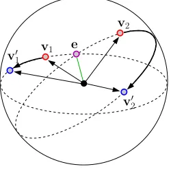
e

Figure 2.9: Image vectors on a sphere with an epipoleefor a pure translation.

is in the epipolar plane containing the two image vectors v and v′. Therefore, a great cirle (plane) joiningvandv′also contains the translation direction vectort.

We now define a property of pure translational motion. Suppose the image vectorsviand

v′_i overlap, as shown in Figure 2.8. Then, for sideways translational motion, the overlapped image vectorsviandv′i will be parallel. On the other hand, in the case of forward motion,vi andv′_iwill meet at a single point. This point is the same as the epipole in the first view.

In other words, this property can also be explained as follows. Suppose the image vectors

v and v′

are on a sphere, as shown in Figure 2.9. The image vectors vand v′

join a plane

(great circle). If there are more than two pairs of matching points such as vi and v ′

i, where

i = 1, . . . , n, and n is the number of point correspondences, then the intersection of these

(34)

v′

2

v2

v′

1

[image:34.612.255.379.113.267.2]

v1

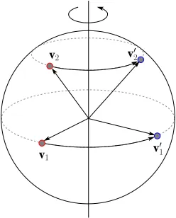
Figure 2.10: Image vectors on a sphere for the pure rotation case.

to estimate the relative orientation of two views.

2.2.4.2 Pure rotation (no translation) case

If the motion of the camera is purely rotational when the two images are captured by the

camera, the geometric relationships ofvandv′can be represented as a simple rotation about an axis, as shown in Figure 2.10.

2.2.4.3 Euclidean motion (rotation and translation) case

If the motion of the camera is both rotational and translational, a general form of the essential

matrixE_{for a pair of matchings points}_v_and_v′_{may be written as follows}5_:

v′ ⊤E_v ₌ _v′ ⊤_[_t_]×Rv (2.14)

= v′ ⊤R_[R⊤_t_]×v (2.15)

= v′ ⊤R_[_c_]_×_v_, _(2.16)

whereR_{is a relative rotation matrix and}_t_{is a translation direction vector. This can be explained}

as rotating the image vectorvin the first view byR_{in order to align the image plane in the first}

view with that in the second view. After all,R_v_{is the image vector in the first image rotated}

into a coordinate system of the second camera.

5

(35)

R_v

c1 e e′ c2

R

X

v′ v

Figure 2.11: Alignment of the first view (indicated in red) with the second view (indicated in blue) in

order to make the two views the same as those in the pure translation case. The virtually aligned view is marked as purple.

As shown in Figure 2.11, on aligning the image planes, the two image planes become

parallel, resulting in a situtation that is similar to the pure translation case. Instead of using the

vectorv, a rotated image vectorR_v_{can be used as the vector corresponding to the image vector}

v. Because the aligned view (indicated in purple) is parallel to the second view (indicated in

blue) as shown in Figure 2.11, the image point vectors v′ and R_v _{also satisfy the epipolar} co-planar constraint as follows:

v′⊤[t]×(Rv) = 0. (2.17)

2.2.4.4 Essential matrix from two camera matrices

Let the two camera matrices beP_{= [}I_|₀_]_andP′_{= [}R_{| −}R_c_{] = [}R_|_t_]_{, where}R_{is the relative} orientation,cis the centre of the second view andt=₋R_c_{is a translation direction vector. As}

explained in the previous section, for a given pair of matching points, vandv′, the essential matrix may be written from the two camera matrices as follows:

v′⊤E_v₌_v′⊤_[_t_]_×R_v_{= 0}_. _(2.18)

(36)

For a general form of two camera matrices such asP₁ _{= [}R₁ _{| −}R₁_c₁_]_andP₂ _{= [}R₂_{| −}

R₂_c₂_]_{, the essential matrix from the general form of two camera matrices may be written as}

follows:

v′⊤E_v₌_v′ ⊤R₂_[_c₁₋_c₂_]×R

⊤

1v= 0. (2.19)

It can be derived from (2.18) by multiplying a4_×4matrix with the camera matricesP₁_and

P₂_{as follows:}

P₁H _{= [}R₁ _{| −}R₁_c₁_]



 

R⊤

1 c1

0⊤ 1





 (2.20)

= [I_|₀_] _(2.21)

and

P₂H _{= [}R₂ _{| −}R₂_c₂_]



 

R⊤

1 c1

0⊤ 1





 (2.22)

= [R₂R⊤

1 |R2c1−R2c2] (2.23)

= R₂R⊤

1[I|R1(c1−c2)]. (2.24)

From (2.21) and (2.24), the essential matrix can be constructed as follows:

E _{= [}R₂₍_c₁₋_c₂_)]×R₂R ⊤

1 (2.25)

= R₂_[_c₁₋_c₂_]_×R⊤

1 . (2.26)

2.2.4.5 Fundamental matrix

The fundamental matrix is basically the same as the essential matrix except that a calibration

matrix is not considered. When calibrated cameras are given, point coordinates in images

are represented in pixel units. However, if we assumme that the cameras are calibrated, we

can eliminate the pixel units by multiplying the inverse of the calibration matrix with the

(37)

directional vectors to the corresponding 3D points. Given calibrated cameras and directional

vectors of the image points, the essential matrix can be easily obtained. On the other hand, if

uncalibrated cameras and pixel coordinates of the image points are provided, we can obtain the

fundamental matrix. Simply, given a point correspondencexandx′ in pixel units, because of the presence of directional image vectorsv =K−1_x_and_v′ ₌K−1_x′_{, where}K_{is a calibration} of the camera, the fundamental matrixF_{may be written as follows:}

v′⊤E_v_{= (}K−1_x′₎⊤E₍K−1_x_{) =}_x′⊤K−⊤EK−1_x₌_x′ ⊤F_x_. _(2.27)

Therefore,F₌K−⊤EK−1_.

Elements of the fundamental matrix Given a fundamental matrixF_{, its elements}F_ij _may

be written as

F=



    

F₁₁ F₁₂ F₁₃

F₂₁ F₂₂ F₂₃

F₃₁ F₃₂ F₃₃



    

. (2.28)

For this F_{, a pair of matching points} _x _{= (}_x₁_{, x}₂_{, x}₃₎_⊤_and _x′ _{= (}_x′

1, x

′

2, x

′

3)

⊤

; hence, the

equation of epipolar constraints can be given as

(x′

1, x

′

2, x

′

3)F(x1, x2, x3)⊤= 0. (2.29)

The coefficients of the termx′

ixjin (2.29) correspond to the elements ofF. These elements of F_{can be determined from two camera matrices and the position of a 3D point using a bilinear}

constraint, which will be explained in the following paragraphs.

Bilinear constraints Let A _and B _{be two camera matrices. Then, a 3D point} _X _{can be}

(38)

non-zero scalar values. These two projections ofXmay be written as



 

A _x ₀

B ₀ _x′

         X −k

−k′

     

=0. (2.30)

If we rewrite (2.30) using the row vectors of the matricesA_andB_{, and the elements of}_x_and_x′_, we can determine the elements of the fundamental matrixF_{. Suppose the two camera matrices}

are A₌       a⊤ 1 a⊤ 2

a⊤₃

      (2.31) and B₌      

b⊤₁ b⊤₂ b⊤₃

      , (2.32)

then, (2.30) is written as

               

a⊤₁ x1

a⊤₂ x2

a⊤₃ x3

b⊤₁ x′

1

b⊤₂ x′

2 b⊤ 3 x ′ 3                       X −k

−k′

      =D       X −k

−k′

     

=0. (2.33)

From the above equation (2.33), the coefficient of the termx′

ixj is determined by

eliminat-ing two rows and the last two columns of the matrixD_{, and by calculating the determinant of}

(39)

§2.3 Estimation of essential matrix 26

as follows:

F_ji _{= (}₋₁₎i+j_det



 

∼a⊤_i

∼b⊤_j





 (2.34)

where_∼ a⊤_i is a2_×3 matrix created after omitting thei-th rowa⊤_i from the matrix A_and ∼b⊤_i is a2_×3matrix is created after omitting thei-th rowb⊤_i from the matrixB_{. Equation}

(2.34) is called a “bilinear relation” for two views. The relations for three and four views are

known as trilinear relations and quadlinear relations, respectively.

2.3 Estimation of essential matrix

2.3.1 8-point algorithm

Longuet-Higgins was the first to develop the 8-point algorithm in computer vision, which

estimates the essential matrix using 8 pairs of matching points across two views [46]. Unlike

Thompson’s iterative method using 5 point correspondences [81], which solves five third-order

equations iteratively, the 8-point method directly obtains the solution from linear equations.

Given the point correspondences v = (v1, v2, v3)⊤ and v′ = (v′1, v

′

2, v

′

3)

⊤

, the 3 _×3

essential matrixE_{can be dervied as follows:}

v′⊤E_v_{= (}_v′

1, v

′

2, v

′ 3)      

E₁₁ E₁₂ E₁₃

E₂₁ E₂₂ E₂₃

E₃₁ E₃₂ E₃₃

            v1 v2 v3      

(40)

A linear equation may be obtained from (2.35) as follows:

(v′₁v1, v

′

1v2, v

′

1v3, v

′

2v1, v

′

2v2, v

′

2v3, v

′

3v1, v

′

3v2, v

′

3v3)

                          E₁₁ E₁₂ E₁₃ E₂₁ E₂₂ E₂₃ E₃₁ E₃₂ E₃₃                          

= 0. (2.36)

It can be observed that equation (2.36) has nine unknowns parameters. However, if we assume

that the value of last coordinate of the matching points is one, for example,v3 = 1and v′3 = 1, the equation has eight unknowns to be solved. Therefore, as there are eight independent

equations for eight pairs of matching points, equation (2.36) can be solved directly.

In order to determine the relative orientation and translation of the camera system from the

estimated essential matrix, Longuet-Higgins proposed a method wherein the translation vector

can be obtained by multiplying the transpose of the essential matrix with (2.18) as follows:

EE⊤ _{= ([}_t_]×R)([t]×R) ⊤

(2.37)

= ([t]×RR

⊤

[t]⊤× (2.38)

= [t]×[t]

⊤

×. (2.39)

If we perform the trace ofEE⊤_{, it becomes Tr}₍EE⊤_{) =}_Tr_([_t_]_×_[_t_]⊤_×_{) = 2}_||_t_||2_{. By assuming}_t to be a unit vector, i.e.,_||t_||= 1, the trace ofEE⊤_{can be given as}

Tr(EE⊤_{) = 2}_. _(2.40)

Therefore, the essential matrix E _{can be normalized by dividing it by}

q

1

2Tr(EE

⊤

(41)

obtaining the normalized essential matrix, the direction of the translation vectortis determined

using the main diagonal ofEE⊤_{as follows:}

EE⊤₌

     

t2₃+t2₂ ₋t2t1 −t3t1

−t2t1 t23+t21 −t3t2

−t3t1 −t3t2 t22+t21

      =      

1₋t2₁ ₋t2t1 −t3t1

−t2t1 1−t22 −t3t2

−t3t1 −t3t2 1−t23

      , (2.41)

wheret2₁ +t2₂+t2₃ = 1because t is a unit vector. From the main diagonal ofEE⊤_{, we can} obtain three independent elements of the translation vectort. However, the scale oftcannot

be determined.

In order to find a relative orientation, Longuet-Higgins used the fact that each row of the

rotation matrix is orthogonal to each row of the essential matrix. Let us suppose qi and ri

are thei-th column vectors of the essential matrixE_{and the rotation matrix}R_{contained in}E_,

respectively. They may be written as

E=

q1 q2 q3

(2.42)

and

R₌

r1 r2 r3

. (2.43)

Then, because [a]×b =a×bsatisfies for any 3-vectoraandb, we can derive the following relations from (2.18) as follows:

qi=t×ri, (2.44)

whereqiis thei-th column vector of the essential matrixE, andriis thei-th column vector of

the rotation matrixR_{, where}_i_{= 1}_{, . . . ,}₃_.

Because ri is orthogonal to qi and is coplanar with t, the vector ri can be written as a

linear combination ofqiandqi×t. If we define a new vectorwi=qi×t, then

(42)

whereλiandµiare any scalar values. Here, the unknown scalarµiis determined to beµi= 1

by substituting (2.45) into (2.44) as follows:

qi = t×ri (2.46)

= t_×(λt+µiwi) (2.47)

= µi(t×wi) (2.48)

= µit×(qi×t) (2.49)

= µiqi. (2.50)

Because the rotation matrixR_{is an orthogonal matrix, the cross products of any two column}

vectors ofR_{are the same as the elements of the remaining column vector of}R_{. For example,}

r1 =r2×r3. Therefore, from (2.46), (2.45) andµ= 1, we obtain

r1 = r2×r3

λ1t+w1 = (λ2t+w2)×(λ3t+w3)

= (λ2t+w2)×(λ3t+w3)

= λ2λ3t×t+λ2t×w3+λ3w2×t+w2×w3

= λ2(t×w3)−λ3(t×w2) +w2×w3

= λ2q3−λ3q2+w2×w3

= λ2q3−λ3q2+ (q2×t)×(q3×t)

= λ2q3−λ3q2+det(q2t t)q3−det(q2t q3)t

= λ2q3−λ3q2+q⊤2(t×t)q3−q⊤2(t×q3)t

= λ2q3−λ3q2−q

⊤

2(t×q3)t.

Because w1, q3 and q4 are all orthogonal to t and the last term on the right in (2.51) is a

multiple oft, the above equation becomes

λ1t=−q

⊤

(43)

On substituting the above equation into (2.45), we obtain the final equation of each column

vector of the roation matrixR_{as follows:}

r1 = w1+w2×w3 (2.52)

r2 = w2+w3×w1 (2.53)

r3 = w3+w1×w2. (2.54)

Although we have estimated the relative orientation and translation using 8 pairs of

match-ing points, there are four possible solutions if we consider signs of the orientations and

trans-lations. In order to identify the signs, Longuet-Higgins proposed a 3D-point reconstruction

method and determined the signs of the translation and rotation on the basis of the values of

the last coordinates of the reconstructed 3D points. If the values of the last coordinates of a

pair of 3D points are negative, then the sign of the translation changes. If the values of the last

coordinates of the 3D points are opposite in sign to each other, then the sign of the rotation is

reversed.

2.3.2 Horn’s nonlinear 5-point method

Horn proposed a method to determine the relative orientation (rotation) and baseline

(transla-tion) of the motion of a camera system using 5 pairs of matching points across the two views

[30]. The rotation of the first camera coordinate system with respect to the second camera is

known as the relative orientation. There are five unknowns parameteres – 3 for rotation and 2

for translation – in the essential matrix.

Given a pair of matching pointsvand v′,R_v_{is the image vector in the first view rotated} into the coordinate system of the right view (or camera), whereR_{is the relative rotation with}

respect to the other view. For these two views, there is a coplanar condition, known as the

epipolar constraint, for the image vectorsR_v_,_v′_{and the translation vector}_t_{as follows:}