Network Structure Optimization with Applications to Minimizing Variance and Crosstalk

(1)

to Minimizing Variance and Crosstalk

Thesis by

Dionysios Barmpoutis

In Partial Fulfillment of the Requirements

for the Degree of

Doctor of Philosophy

California Institute of Technology

Pasadena, California

2012

(2)

c ⃝2012

Dionysios Barmpoutis

(3)

(4)

Acknowledgments

As I near the end of my time at Caltech, I can’t help but reflect back on all the

people who have helped me along the way. I have had the pleasure of working with

many amazing individuals, both students and faculty. First and foremost, I would

like to thank my advisor, Richard M. Murray. His energy and passion have been a

source of inspiration throughout my graduate career at Caltech. With his guidance

and mentorship, I have grown as a student, as a researcher, and as a person. All his

insightful comments were greatly appreciated, and his ability to guide me while still

allowing me to have control of the direction of my research projects created great

opportunities along the way. I would also like to thank Yaser Abu-Mostafa, Joel

Burdick, John Doyle, and Pietro Perona, for their advice and for generously taking

the time to be part of my thesis committee.

For our many meaningful discussions, I would like to thank my officemate, Chris

Kempes. I would also like to thank Sotiris Masmanidis, one of the first people I

worked with at Caltech, for his leadership and advice. There are many other

individ-uals who have made my time at Caltech fulfilling both academically and personally,

and for that, I would like to extend a big thanks to Elisa Franco, Theodoros

Dikalio-tis, Vanessa J¨onsson, Ophelia Venturelli, Andy Lamperski, H˚akan Terelius, Chess

Stetson, Sawyer Fuller, Dan Wilhelm, Alice Robinson, Shaunak Sen, Molei Tao,

Paul Skerritt, Costas Anastassiou, Joe Meyerowitz, Xiaodi Hou, Pete Trautman,

Vasileios Christopoulos, Shuo Han, Andrea Censi, Aristo Asimakopoulos, Jongmin

Kim, Stephen Prajna, Mumu Xu, Jun Liu, Demetri Spanos, Chris Santis, Eyal En

(5)

not have been possible without the academic guidance I received from Erik Winfree,

Shuki Bruck, Paul Rothemund, and Christof Koch. It has truly been an honor to

have known and worked with all of them during my graduate studies.

I was also very fortunate to have entered Caltech with such great people in the

CNS class in the Fall of 2007: Julien Dubois, Virgil Griffith, Alice Lin, Akram Sadek,

Marie Suver, and Peter Welinder. It was a great pleasure spending time together

working through our problem sets during our first year of classes. In addition to the

support I received from fellow students and faculty, I must thank Anissa Scott and

Gloria Bain for making my life so much easier with booking flights, preparing for

conferences, and assisting with other administrative issues.

Of course, I am forever grateful to my parents and brother for their unconditional

support, even while being thousands of miles away. Last but not least, I would like to

thank Alison Rose for her unconditional love and constant support through the ups

(6)

Abstract

This thesis provides a unified methodology for analyzing structural properties of

graphs, along with their applications. In the last several years, the field of

com-plex networks has been extensively studied, and it is now well understood that the

way a large network is built is closely intertwined with its function. Structural

prop-erties have an impact on the function of the network, and the form of many systems

has been evolved in order to optimize for given functions. Despite the great progress,

particularly in how structural attributes affect the various network functions, there is

a significant gap in the quantitative study of how much these properties can change

in a network without a significant impact on the functionality of the system, or what

the bounds of these structural attributes are. Here, we find and analytically prove

tight bounds of global graph properties, as well as the form of the graphs that achieve

these bounds. The attributes studied include the network efficiency, radius, diameter,

average distance, betweenness centrality, resistance distance, and average clustering.

All of these qualities have a direct impact on the function of the network, and finding

the graph that optimizes one or more of them is of interest when designing a large

system. In addition, we measure how sensitive these properties are with respect to

random rewirings or addition of new edges, since designing a network with a given set

of constraints may include a lot of trade-offs. This thesis also studies properties that

are of interest in both natural and engineered networks, such as maximum immunity

to crosstalk interactions and random noise. We are primarily focused on networks

where information is transmitted through a means that is accessible by all the

(7)

comprise it do not necessarily have a dedicated mechanism that facilitates

informa-tion transmission, or isolates them from other parts of the network. Two examples

of this class are biological and chemical reaction networks. Such networks suffer from

unwanted crosstalk interactions when two or more units spuriously interact with each

other. In addition, they are subject to random fluctuations in their output, both due

to noisy inputs and because of the random variance of their parameters. These two

types of randomness affect the behavior of the system in ways that are intrinsically

different. We examine the network topologies that accentuate or alleviate the effect

of random variance in the network for both directed and undirected graphs, and find

that increasing the crosstalk among different parts reduces the output variance but

(8)

List of Figures

3.1 Examples of networks with the minimum distance . . . 25

3.2 Type I and typeII almost complete graphs . . . 26

3.3 Networks with the largest average distance . . . 31

3.4 Upper and lower bounds for the average distance of networks . . . 37

3.5 Upper and lower bounds on the efficiency of networks . . . 46

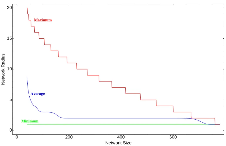
3.6 Structure of networks with the largest radius . . . 51

3.7 Upper and lower bounds on the average radius of networks . . . 54

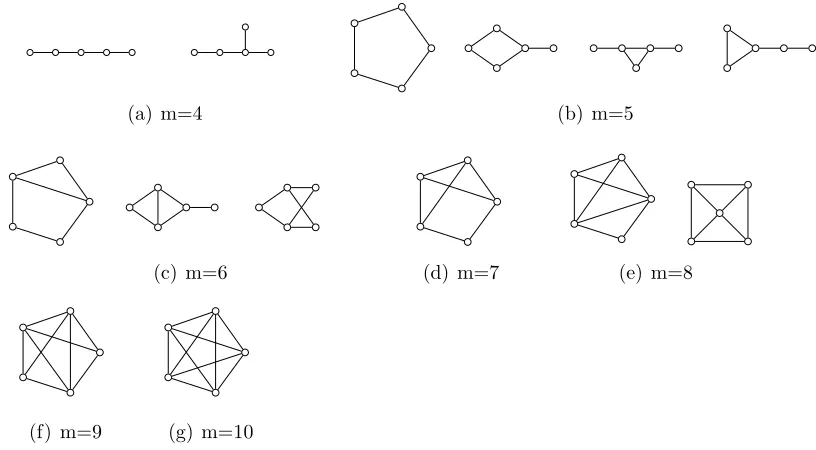
3.8 Examples of networks with the largest radius . . . 55

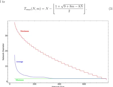
3.9 Upper and lower bounds on the diameter of networks . . . 58

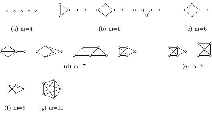
3.10 Examples of networks with the largest diameter . . . 60

3.11 Networks with the largest radius that do not have the largest diameter and vice versa . . . 61

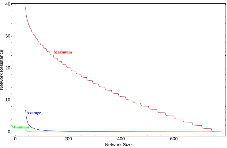
3.12 Resistance of almost complete graphs . . . 65

3.13 Upper and lower bounds on the average resistance of networks . . . 67

3.14 Definition of clustering coefficient . . . 70

3.15 Graphs with one vertex connected to a clique . . . 73

3.16 Clustering for the almost complete graphs . . . 75

3.17 Increasing the resilience of graphs against vertex removal . . . 87

3.18 Alternative definition of clustering coefficient for vertices with degree one 89 3.19 Graphs of order 10 and all sizes with the largest average clustering . . 90

(13)

3.21 Standard deviation of various graph properties as a function of the

net-work size . . . 94

3.22 Evolution of the average distance, radius, diameter, and resistance of

networks after successive random rewirings . . . 96

3.23 Sensitivity of the clustering coefficient to random rewirings . . . 97

4.1 Double rewirings are needed in order to reduce crosstalk sensitivity . . 112

4.2 Nonisomorphic subgraphs of degree 4 and partially defined connectivity 113

4.3 The rewiring algorithm cannot be trapped in a local minimum . . . 116

4.4 All connected graphs of orderN = 6 with the smallest crosstalk sensitivity119

4.5 An example of the overall vertex affinity function . . . 119

4.6 Type I almost complete graph and a transformation that preserves the

degree sequence . . . 121

4.7 All connected graphs of order N = 6 with the smallest overall crosstalk

sensitivity (Multiplicative crosstalk) . . . 127

4.8 Bounds on the minimum overall crosstalk sensitivity . . . 130

4.9 A rewiring method that keeps the degree of each vertex constant . . . 132

5.1 Variance of the output of a unidirectional and a bidirectional serial

path-way as a function of the pathpath-way length . . . 151

5.2 Covariance and correlation among all pairs of nodes in a linear pathway 152

5.3 Average variance of all nodes in a network in a cycle as compared to an

identical network without the feedback loop . . . 153

5.4 A network consisting of a feedforward cycle and the corresponding noise

strength in its output . . . 154

5.5 Correlations increase the variance in bidirectional networks . . . 155

5.6 A serial pathway with a unit feedback loop . . . 156

5.7 Output variance of a linear pathway with a positive or negative

(14)

5.8 All connected networks of order N = 6 and minimum output variance . 162

5.9 A simple electrical circuit with two noise sources . . . 163

5.10 Crosstalk topologies involving one network node . . . 165

5.11 Output variance as a result of noise input for a single vertex in the

network and the existence of crosstalk interactions with other vertices . 168

5.12 Normalized variance of the output when the crosstalk introduces

addi-tional noise . . . 168

5.13 Output noise of two parallel pathways with crosstalk between each other 169

5.14 Output variation for each node in a system ofN nodes, when there are

crosstalk interactions among every pair of nodes . . . 171

5.15 Comparison of the output noise intensity of a simple network with direct

and indirect crosstalk interactions . . . 173

5.16 Output variance of a single pole filter as a function of time when the

(15)

List of Tables

4.1 Possible degree orders of a subgraph of order 4, and the respective

dif-ference in crosstalk after rewiring . . . 114

4.2 All degree orders of a subgraph of order 4, and crosstalk difference after

(16)

Chapter 1 Introduction

1.1 Motivation

The area of complex networks has seen an explosion in the last several years. Many

properties of large scale networks have been studied extensively, along with their

applications to engineering and biology [1, 8, 34, 37, 40, 45]. However, there have been

relatively few studies so far on the bounds of the structural properties of networks.

The purpose of discovering these bounds is twofold. First, these bounds will give

a clear measure of the importance of each property, especially relative to the others,

as well as their trade-offs. If for example a natural network has a clustering coefficient

that is very close to the theoretical maximum, it means that the clustering coefficient

provides some advantage, or that it is correlated with some other property that is

important for the function of the network. Otherwise, natural evolution would force

it to drift to an average value. In addition, since several of the properties of the

network require different or even contradicting topologies, usually there are limits on

how much of each property a network may have. Knowing where these trade-offs lie

can give us a clear picture of how important each property is relative to the others.

The second reason is for optimizing the way individual elements of a network

are connected and how they communicate, especially on a large scale. Knowing the

(17)

it will be easier to optimize its function or design it in such a way that all constraints

are simultaneously satisfied with the given trade-offs. In biological and chemical

reaction systems, there is yet another compelling reason: Since the structure of a

natural system has been shaped by evolution, we have the chance to see the interplay

between structure and evolvability, and how they affect each other [19, 35, 50], or

even find evidence of different environmental conditions that may have shaped it [36].

On a different note, bioengineers have long started building simple biological

net-works, both as part of the cell [24] and in vitro [25, 38], but despite the many efforts,

they remain relatively small so far [57, 58], especially compared with the natural

networks, which are orders of magnitude larger and more complex [71]. Two likely

reasons why engineering biological circuits is so difficult are the unwanted physical

interactions among unrelated molecules, and the fact that noise is often times much

stronger than the signal itself.

Biological networks make use of a variety of strategies in order to reduce noise,

and to increase the robustness to random changes, but these mechanisms may be

used for many different purposes, and are not yet well understood [39, 71]. The

ones that sense the environment and process the information received are usually

implemented by changing the number of molecules that are specific to each function.

More generally, in networks where the different parts are free to physically move

in a solution, and where interactions between different molecules require them to

come in contact, there are many unmodeled interactions, since there are no dedicated

information-transmitting mechanisms. Everything depends on physical presence of

molecules, which is by definition random and displays significant internal noise [55].

Relations between different entities may also depend on their physical shape, and the

different molecules that constitute the network may have compatible shapes, making

interactions easier. As a result, many molecules temporarily form complexes that

seem to serve no purpose, and in addition, prevent the respective molecules from

(18)

Another problem is that these kinds of systems are very prone to noise from many

different sources [54, 56]. Although noise has been shown to be a feature and not a

drawback in some cases [23], it is usually detrimental to the function of the network,

since it may reduce its reliability and accuracy in reading external stimuli, or reacting

to environmental inputs. Both of these problems are accentuated when there are few

molecules of each type and there are many types of each molecule, as actually happens

in most biological systems, and the number of molecules of each type cannot be a

continuous variable, making accuracy and reliability even harder to achieve [54]. In

certain contexts, it has also been shown that noise imposes limits to the accuracy of

a biological network [42].

In this thesis, we tackle both aforementioned problems from a network perspective.

We first find the extremal properties that are of interest in the function of many

networks, and then we study the structure that optimizes them. Then, we design

networks that minimize crosstalk and maximize noise immunity. We also study in

detail how noise propagates in such networks. Finally, we distinguish between two

types of variance sources that contribute to a nondeterministic output, the first being

the noise in the inputs, and the second being variance in the network parameters.

These two types of variance affect the network outputs in fundamentally different

ways.

1.2 Thesis Outline and Contributions

Chapter 2 introduces some basic notions and definitions from network theory,

stochas-tic calculus, and dynamical systems theory that will be used throughout this thesis.

It also revisits some properties of graphs, Wiener processes, and linear dynamical

systems that will be used in later chapters.

Chapter 3 focuses on theoretical results regarding the structural characteristics of

(19)

along with methods on how to build the networks that achieve these bounds. We

describe the structure of connected graphs with the minimum and maximum average

distance, radius, diameter, betweenness centrality, efficiency and resistance distance,

and average clustering, given their order and size. We find tight bounds on these

graph qualities for any arbitrary number of nodes and edges and analytically derive

the form and properties of such networks. We determine if a graph with one or more of

these extremal properties is unique or not, depending on the property and the graph’s

order and size. We also measure the sensitivity to rewiring of each architecture, and

how robust each structure is with regard to changes in the graph.

Chapters 4 and 5 are devoted to the study of networks where information is

trans-mitted through a means that is accessible by all the individual units of the network.

Such networks include biological and chemical reaction networks, where all reactions

take place in a solution in which all molecules may physically interact with all

oth-ers, based on their physical proximity. Crosstalk is defined as the set of unwanted

interactions among the different constituents of the network and is present in

vari-ous degrees in every such system. Using concepts from graph theory, we introduce

a quantifiable measure for sensitivity to crosstalk, and analytically derive the

struc-ture of the networks in which it is minimized. It is shown that networks with an

inhomogeneous degree distribution are more robust to crosstalk than corresponding

homogeneous networks. We provide a method to construct the graph with the

min-imum possible sensitivity to crosstalk, given its order and size. For networks with a

fixed degree sequence, we present an algorithm to find the optimal interconnection

structure among their vertices.

In Chapter 5, we describe how noise propagates through a network. Using

stochas-tic calculus and dynamical systems theory, we study the network topologies that

ac-centuate or alleviate the effect of random variance in the network for both directed

and undirected graphs. Given a linear tree network, we show that the variance in

(20)

eas-ily be optimized with existing techniques [17]. Cycles create correlations which in

turn increase the variance in the output. Feedforward and feedback have a limited

effect on noise propagation when the respective cycle is sufficiently long. Crosstalk

between the elements of different pathways helps reduce the output noise, but makes

the network slower. Next, we study the differences between disturbances in the inputs

and disturbances in the network parameters, and how they propagate to the outputs.

Finally, we show how noise correlation can affect the steady state of the system in

chemical reaction networks with reactions of two or more reactants, each of which

may be affected by independent or correlated noise sources.

Chapter 6 concludes the analysis by giving an overview of the results presented

(21)

Chapter 2 Background and Preliminaries

This chapter provides a brief introduction to the mathematical preliminaries that will

be used throughout this thesis. We will revisit some basic definitions and properties

from graph theory, linear control systems, and stochastic calculus.

2.1 Graph Theory

A graph (also called a network) is an ordered pair G = (V,E) comprised of a set V = V(G) of vertices together with a set E = E(G) of edges that are unordered 2-element subsets ofV. Two verticesu andv are calledneighbors if they are connected through an edge ((u, v)∈ E) and in this case we writeu−v, otherwise we writeu /−v. A graph issimple when all edges connect two different vertices, there is at most one edge connecting any pair of vertices, and edges have no direction. A weighted graph associates a weight with every edge. In this thesis, when a graph is weighted, all

weights will be restricted to positive real numbers. The neighborhood Nu of a vertex

u is the set of its neighbors. The degree of a vertex is the number of its neighbors. A vertex is said to have full degree if it is connected to every other vertex in the network.

A network is assortative with respect to its degree distribution when the vertices with large degrees are connected to others that have large degrees and vertices with

(22)

small degrees connect to vertices with large degrees and vice versa, then the network

is called disassortative. The order N = N(G) of a graph G is the number of its vertices, N = |V(G)|. A graph’s size (denoted by m =|E(G)|), is the number of its edges. We will denote a graph G of order N and size m as G(N, m) or simply GN,m. A complete graph is a graph in which each vertex is connected to every other. The edge density of a graph is defined as ρ=m/(N₂), representing the number of present edges, as a fraction of the size of a complete graph, which is the total number of

vertex pairs. Aclique in a graph is a subset of its vertices in which every vertex pair in the subset is connected. The clique order is the number of vertices that belong to it. A clique that consists of three vertices (and three edges among them) is called a

triangle. A path is a sequence of consecutive edges in a graph and the length of the path is the number of edges traversed. A path with no repeated vertices is called a

simple path. Atree is a graph in which any two vertices are connected by exactly one path.

The distance between two vertices u and v (usually denoted by d = d(u, v)), is the length of the shortest path that connects these two vertices. A cycle is a closed (simple) path, with no other repeated vertices or edges other than the starting and

ending nodes. A cycle is called chordless when there is no edge joining two nodes that are not adjacent in the cycle. Afull cycle is a cycle that includes all the vertices of the network. A graph G is connected if for every pair of vertices u ∈ V(G) and

v ∈ V(G), there is a path from u to v. Otherwise the graph is called disconnected. We will be focusing exclusively on connected graphs, since every disconnected graph

can be analyzed as the sum of its connected components. If the distance between u

and v is equal to k, then these vertices are calledk-neighbors, and the set of all pairs in the graph that are k−neighbors is denoted by Ek. The eccentricity of a vertex u

is the maximum distance of u from any other vertex in the graph. A central vertex of a graph is a vertex that has eccentricity smaller or equal to any other node. A

(23)

eccentricity of a central vertex is called the graph radius. The graph diameter is defined as the maximum of the distances among all vertex pairs in the network.

A cut is a partition of the vertices of a graph into two disjoint subsets. A cut set of the cut is the set of edges whose end points are in different subsets of the cut. A cut vertex of a connected graph is a vertex that if removed, (along with all edges incident to it) produces a graph that is disconnected. An edge is rewired when we change the vertices it is adjacent to. A single rewiring takes place when we change one of the vertices that is adjacent to it, and adouble rewiring occurs when we change both of them. A subgraph H of a graph G is called induced if V(H) ⊆ V(G) and for any pair of vertices u and v in V(H), (u, v) ∈ E(H) if and only if (u, v) ∈ E(G). In other words,H is an induced subgraph ofG if it has the same edges that appear inG over the same vertex set. Furthermore, if the vertex set ofH is the subsetS ofV(G), then H can be written as G[S] and is said to be induced by S. Finally, two graphs G and H are called isomorphic if there exists a bijective function f : V(G) → V(H) such that

(u, v)∈ E(G) ⇐⇒ (f(u), f(v))∈ E(H). (2.1)

Two graphs that are isomorphic have by definition the same order and size, and are

considered identical. A thorough treatment of the graph theory notions can be found

in any introductory graph theory text, including [31] and [48].

2.2 Wiener Processes

In this section, we will be describing some elementary properties of the Wiener process

that will be used. Letξn, n∈N be a sequence of independent identically distributed random variables with zero mean and unit standard deviation. Their sum is

Sn = n

∑

k=1

(24)

We now define the piecewise constant function

Wt = lim n→∞

S_⌊nt⌋ √

n (2.3)

with t ∈ R+. According to the Central Limit Theorem, the distribution of Wt is independent of the distribution of the sequence of ξn, as long as they have finite variance, and are identically distributed and independent of each other. The random

process Wt is normally distributed with variance equal to the time interval it which it is measured:

Wt= lim n→∞

S_⌊nt⌋ √

nt

√

nt

√

n =⇒ Wt ∼ N(0, t). (2.4)

The difference of two sumsSb−Sawitha < bhas the same distribution of the random variable Sb−a and as a result

Wb−Wa∼Wb−a 0≤a < b. (2.5)

Lastly, the random variablesWb−WaandWd−Wcare independent when 0≤a < b≤

c < d, since the respective sums consist of independent random variables. More details

on the properties of the Wiener process can be found in [44]. An excellent treatment

of stochastic methods in physics, chemistry, and biology, along with examples, can

be found in [26].

2.3 General Response of Linear Systems

In this section, we briefly revisit some basic tools from control systems theory.

Con-sider a linear time invariant system with impulse response h(t, s). The general form

of the output when the input signal is u(t) is

y(t) =

∫ t

−∞

(25)

where h(t, s) is the impulse response of the dynamical system [6]. A system with m

inputs, n states, and p outputs can be written in the form

S :

              

dx

dt =Ax+Bu

y=Cx,

(2.7)

where the dimensions of matricesA,B, andCaren×n,n×m, andp×n, respectively. We will always assume that the systems we study are stable, which in this context

means that theAmatrix has eigenvalues with strictly negative real parts. The output

of the system at time t when the input is an impulse applied at time s is

h(t, s) = CeA(t−s)B (2.8)

and equation (2.6) can be simplified to

y(t) =C

∫ t

−∞

eA(t−s)Bu(s)ds. (2.9)

When the network in question is comprised of elements whose outputs obey linear

time-invariant differential equations, we can also find the Fourier transform of the

network output:

H(ω) =

∫ +∞

−∞

h(t)e−jωtdt, (2.10)

whereh(t) = h(t,0) is the impulse response of the system andω = 2πf is the angular

frequency. If the system is causal (h(t) = 0 for t <0), then the expression above can

be simplified by replacing the lower limit of the integral with zero.

When the input is a stationary stochastic process, its output will be a stochastic

process as well. We are interested in the mean, the variance, and occasionally the

(26)

equi-librium state. The mean E[y(t)] and the variance V[y(t)] of the output y(t) in the

steady state will be denoted as E[y] and V[y], respectively:

E[y] = lim

t→∞E[y(t)] and V[y] = limt→∞V[y(t)]. (2.11)

If we know the impulse response of the system, the mean of the output vector can be

expressed as

E[y(t)] =E

[∫ t

−∞

h(t−s)u(s)ds

]

=

∫ t

−∞

h(t−s)·E[u(s)]ds,

(2.12)

where in the last equation we have interchanged the expectation with the integration

operator, assuming that the input functions are non-pathological, and the quantities

are finite, such that all the integrands are measurable in the respective measure

space (Fubini’s theorem, [44]). In what follows, we will always assume that all such

conditions are satisfied. Furthermore, we will disregard any nonzero mean values in

the outputs when the system is linear. The covariance matrix of the outputs, when

applying the same input, is

V[y(t)] =E[y(t)·yT(t)]−E[y(t)]·E[yT(t)]

=

∫ t

−∞

∫ t

−∞

h(t−r)(E[u(r)uT(s)]−E[u(r)]E[uT(s)])hT(t−s)drds.

(2.13)

Assuming that u(t) = 0 for t <0, and according to equation (2.11),

V[y] = lim t→∞

∫ t

0

∫ t

0

h(t−r)(E[u(r)uT(s)]−E[u(r)]E[uT(s)])hT(t−s)drds.

(27)

Chapter 3 Extremal Properties of Complex

Networks

3.1 Introduction

Complex networks, as abstract models of large dynamical systems, match the

struc-ture of real-world networks in many diverse areas. These include both natural and

engineered systems such as gene regulation, protein interaction networks, food webs,

economic and social networks and the internet, to name a few (see [65] and references

therein). Complex systems can be described as interconnections of simpler elements,

which in turn can be analyzed abstractly as graphs.

In this chapter, we are interested in the structural properties of networks,

regard-less of the nature of their individual parts. This allows the results developed here to

be applicable in a wide range of different disciplines, such as neuroscience, biology,

social sciences, and engineering. The properties studied are of general interest, since

many network functions are sensitive to them: the average distance, betweenness

centrality, radius, diameter, efficiency, graph resistance, and average clustering.

De-pending on the application, we usually want to minimize or maximize one or more

of the above, because they are directly implicated in some performance metric of the

network. They are correlated with how fast the system responds to different input

(28)

ran-dom failures or targeted attacks [1, 18, 28]. They also indicate how efficient message

propagation is across a network [7, 41], how easy it is for dynamical processes that

require global coordination and information flow (like synchronization or

computa-tion) to take place, and how reliable a transmitted message is in the presence of noise

[65]. Although these structural properties do not take into account the specifics of

the various systems, focusing on the structural patterns of the network topology can

give a valuable insight on how to optimize the network function, while obeying other

limitations. In general, networks need to obey many different constraints, and taking

into account all of them may result in different optimal structures, depending on the

importance (weight) given to each constraint [14].

3.2 Networks with the Minimum and Maximum

Average Distance

3.2.1 Minimum Average Distance

The average distance of a network is an important property, since it is a direct

indica-tor of how different parts of the network communicate, and exchange information. A

small average distance is a proxy for improved synchronizability, efficient computation

and signal propagation across the network [65]. In this section, we will analytically

compute the minimum average distance of a graph of fixed order and size, and find

sufficient conditions in order to achieve that minimum.

Lemma 1. If two connected graphs Gand H with V(G) =V(H)have edge sets E(G) andE(H), respectively, such that E(G)⊆ E(H), thenD¯(G)≥D¯(H), where D¯ denotes the average distance of the graph.

Proof. If we start with graphG =G(N, m) with average distance ¯D(G), and introduce one additional edge, the new graph G′ = G′(N, m+ 1) will have an average distance

¯

(29)

previously non-neighboring vertices s and t, changing their distance to d′(s, t) = 1.

Since they were not connected before, their distance was d(s, t) ≥ 2, so d′(s, t) < d(s, t). For every other pair of vertices u and v, the new edge can only create new

shortest paths, so d′(u, v) ≤ d(u, v). The total average shortest path length of the new graph is:

¯

D(G′) = (_N1

2

) ∑

(u,v)∈V2₍_G′₎

u̸=v

d′(u, v)< (_N1

2

) ∑

(u,v)∈V2₍_G₎

u̸=v

d(u, v) = ¯D(G). (3.1)

Adding new edges as above, we can start from graph G, and successively construct the graph H, which will have a strictly smaller average distance.

Lemma 2. The star graph is the only tree of order N that has the smallest average distance equal to D¯star = 2− _N2.

Proof. A tree has exactly N −1 edges among its N vertices. There will be exactly

N − 1 pairs of vertices with distance d = 1, and (N₂−1) vertex pairs that are not connected, with distances d(u, v)≥2. The star graph achieves this lower bound, and has the minimum possible average distance.

¯

Dstar = 1

(_N

2

) ∑

(u,v)∈V2

u̸=v

d′(u, v) = (_N1

2

) (

N −1 + 2

(

N −1 2

))

= 2− 2

N. (3.2)

It is also unique: If a tree is not a star, there is no vertex that is connected to all the

remaining vertices. In this case, there are at least two vertices with distance d ≥3, since in every tree there is a unique path connecting each vertex pair, and at the same

time the number of neighboring vertices is the same as in the star graph.

Using the same method as above, we can find the smallest average distance of a

graph with N vertices andm edges, which we denote as ¯Dmin(N, m).

Theorem 1. The minimum possible average distance of a graph G(N, m) is equal to ¯

Dmin(N, m) = 2− ₍mN

2)

(30)

Proof. The graph G(N, m) has m pairs of vertices with distance exactly 1, and the rest of the pairs of vertices (u, v) have distancesd(u, v)≥2. Consequently, its average distance is

LG≥

m+ 2((N₂)−m)

(_N

2

) = 2−(m_N

2

). (3.3)

This lower bound can always be achieved. A connected graph G(N, m) with at least one vertex with degree d=N −1 has the star graph as an induced subgraph, so all non-neighboring vertices will have distance equal to 2. All connected vertices have

distance equal to 1, leading to the lower bound of equation (3.3).

Corollary 1. If a graphG has at least one vertex pair(u, v)with distanced(u, v)≥3, then its average distance is L_G >D¯min(N, m).

Proof. The number of pairs with distance 1 is fixed, equal to the graph’s size. All other vertices have a distance of at least 2, and the minimum is achieved when all non-neighboring pairs have distance equal to 2.

The next three corollaries present sufficient conditions for a graph to have the

smallest average shortest path length.

Corollary 2. In a network with the smallest average distance, all vertex pairs are either connected, or connected to a common third vertex.

Proof. From Corollary 1, all vertices that are not connected through an edge have distance equal to 2, which means that they have a common neighbor.

Corollary 3. A cut of a minimum average distance graph G divides its vertices into two disjoint sets where, in at least one of the sets, all vertices have at least one neighbor in the other.

Proof. Assume that in both sets of a graph G there is at least one vertex which has no neighbors to the other set. The distance between these two vertices is at least

(31)

Corollary 4. Assume that the graph G of order N has the smallest average distance. The average degree ¯g_Nu of the neighbors of vertex u which has degree equal to du satisfies the inequality

¯

g_Nu ≥ N −1 du

. (3.4)

Proof. Since every vertex u of G has distance exactly 2 with all its non-neighbors, the vertices in its neighbor set Nu = {V1, . . . , Vdu} should be connected to all the

remaining vertices. In other words, all the remainingN−1−du vertices of the graph should have at least one common neighbor withu. Each neighborVk ofuwith degree

gk has gk−1 neighbors other than u, some of which may belong toNu. If we sum up the number of neighbors of all these vertices (excludingu), we get:

∑

k∈Nu

(gk−1)≥N −1−du

∑

k∈Nu

gk≥N −1

dug¯_Nu ≥N −1 ¯

g_Nu ≥ N −1 du

.

(3.5)

Corollary 5. Networks that have the smallest possible average shortest path length are disassortative with respect to their degrees.

Proof. It follows directly from equation (3.5) and the definition of a disassortative network.

(32)

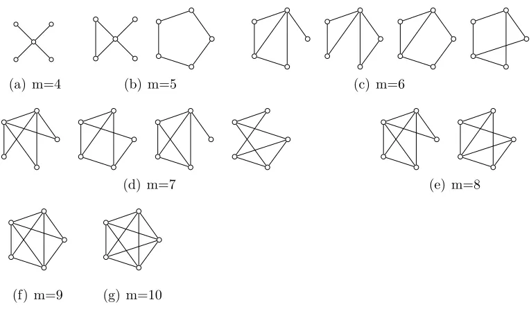
(a) m=4 (b) m=5 (c) m=6

(d) m=7 (e) m=8

[image:32.612.133.516.100.323.2]

(f) m=9 (g) m=10

Figure 3.1: All connected networks with 5 vertices and 4≤m≤10 edges with the smallest average shortest path length. In these graphs, all nodes that are not connected are second neighbors.

3.2.2 Maximum Average Distance

The networks with the largest average distance have a very different topology. They

consist of two distinct connected subgraphs, and if we remove any edge, the network

either becomes disconnected, or the previously connected vertices become second

neighbors.

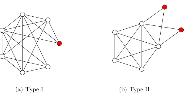
Definition 1. We call a connected graph of order N and size m almost complete when its largest clique has order N −1 or N −2. We distinguish these two cases by calling them type I and type II, respectively. In order to be almost complete, a graph needs to have (N₂−1)+ 1 ≤ m ≤ (N₂)−1 (type I), or (N₂−2)+ 2 ≤ m ≤ (N₂−1) (type II) edges. The vertices of the largest clique are called central vertices, whereas the vertices not belonging to it are called peripheral vertices.

(33)

[image:33.612.173.476.97.254.2]

(a) Type I (b) Type II

Figure 3.2: (a) The type I almost complete graph consists of a clique of N −1 vertices, and one peripheral vertex (shown in red) that connects to them. (b) The type II almost complete graph of order N consists of a clique of order N −2, and two additional vertices that connect to it (and possibly to each other).

Lemma 3. Assume that a vertex u with degree du is added to a network, with its neighbor set being Nu. Rewiring edges of G such that they connect previously non-neighboring vertices in Nu cannot decrease its eccentricity or the average distance of

u with the other vertices in the network.

Proof. Connecting any two vertices in Nu will not change the distance of u with any of them. Furthermore, disconnecting a pair of vertices, at least one of which is not in

Nu, can only increase the distance of uwith any of the vertices that do not belong to the set of its neighbors.

More generally, connecting two non-neighboring vertices has the smallest impact

on their average distance if they have a common neighbor. Rewiring an edge inG will increase the distance of the initially connected pair (u1, v1) to d (where d ≥ 2), and

(34)

1. The overall difference will be

∆d(u1, v1) + ∆d(u2, v2) = (dnew(u1, v1)−dold(u1, v1))

+ (dnew(u2, v2)−dold(u2, v2))

=d−2 ≥0.

(3.6)

Combining Lemma 3 with equation (3.6), we can easily see that for a fixed

neigh-borhoodNu of a vertexu, we can increase the eccentricity of u and at the same time the average distance of the graph it belongs to, simply by rewiring edges to connect

vertices in Nu, until they form a clique.

Lemma 4. All connected graphs of order N ≥2 and size(N₂−1)+ 1≤m≤(N₂) have the same average distance, equal to

¯

D(N, m) = 2−(m_N

2

). (3.7)

Proof. Assume that the largest clique in G consists of C vertices, which we will call central vertices. The rest of the nodes belong to the setP ofperipheral vertices, with |P|=P and they may form connections to the central vertices and among themselves. Since m ≥ (N₂−1)+ 1, every vertex in the graph is either a central or a peripheral vertex, and as a result

C+P =N. (3.8)

The average distance of equation (3.7) is equal to the minimum possible distance of a

graph as in equation (3.3), and it is achieved if and only if all non-neighboring vertices

have distance equal to 2. The only way that the network will not have an average

(35)

Corollary 1 we conclude that the maximum average distance of the graph will be

D(G)>2− (m_N

2

). (3.9)

The central vertices are by definition fully connected to each other, and any peripheral

vertex has distance two with all the central vertices it is not connected with. So, the

only case where two non-neighboring vertices do not have any common neighbors is

when both of them are peripheral vertices. We will now show that this is not possible.

For every peripheral vertexu, there areγu central vertices that arenot connected to it. Also, let h be the total number of non-neighboring peripheral vertices. The

total number of non-neighboring vertex pairs is

γ =h+∑

u∈P

γu (3.10)

with

γ =

(

N

2

)

−m

≤

(

N

2

)

−

(

N −1 2

)

−1

=N −2.

(3.11)

In addition,

h≥1 (3.12)

since A and B are not connected. Combining all the equations above:

h+∑

u∈P

γu ≤N −2 =⇒

∑

u∈P

γu ≤N −3

=⇒ γA+γB+

∑

u∈P u̸=A,u̸=B

γu ≤N −3.

(3.13)

(36)

to, so

γu ≥1 ∀u∈ P (3.14)

and

∑

u∈P u̸=A,u̸=B

γu ≥P −2. (3.15)

Based on the last two inequalities combined with inequality (3.13), we can derive an

upper bound for the sum of γA and γB:

γA+γB ≤N −P −1 ≤N −3

(3.16)

becauseP ≥2. ButAand B have by assumption no common neighbors in the clique or among any peripheral vertices, which means that

γA+γB ≥N −2 (3.17)

which is clearly a contradiction.

Corollary 6. There are exactly

⌊

N−2 2

⌋

non-isomorphic graphs of order N and size

m=(N₂−1) with the largest possible average distance, equal to

¯

Dmax(N, m) = 2−

m−1

(_N

2

) . (3.18)

All other graphs of the same order and size have the minimum possible average dis-tance among their vertices, equal to

¯

Dmin(N, m) = 2−

m

(_N

2

). (3.19)

(37)

the pairs of vertices is

γ =

(

N

2

)

−

(

N −1 2

)

=N−1. (3.20)

Keeping the same notation as before, we sum up all the missing edges among the

peripheral vertices, and among peripheral and central vertices.

h+γA+γB+

∑

u∈P u̸=A,u̸=B

γu =N −1 (3.21)

under the constraints

γA+γB ≥N −P,

∑

u∈P u̸=A,B

γu ≥P −2 and h≥1. (3.22)

These inequalities can only be satisfied in equation (3.21) if all variables are equal to

their respective lower bounds, namely

γA+γB =N −P,

∑

u∈P u̸=A,B

γu =P −2 and h= 1. (3.23)

The only unknown variable above is P. Since A and B are not neighbors, there is

only one (h = 1) edge missing among peripheral vertices. If we assume that P ≥3, then A and B have exactly P −2 common neighbors, which are peripheral vertices that are connected to both of them. This would clearly contradict our assumption.

Consequently, A and B are the only peripheral vertices and P = 2. Such a graph is

shown in Figure 3.3(a). It is clear from the previous analysis that

dA+dB+γA+γB = 2(N −2) =⇒ dA+dB =N −2 (3.24)

(38)

A B Peripheral Vertices

dA dB

(N-2)-Complete Graph

[image:38.612.129.522.98.235.2]

(a) (b)

Figure 3.3: (a) A network with size m = (N₂−1) and largest possible average distance. VerticesAandB are the only vertices without any common neighbors, anddA+dB=N−2, the number of central vertices. (b) The graph of orderN = 12 and size m= 24, with the largest average shortest path length. It consists of a complete graph of order C= 6 (blue), and a path graph of orderP =N−C= 6 (green). Four edges (α= 4) connect the complete subgraph to one of the two ends of the path graph.

only the non-isomorphic graphs, it is clear that there are exactly ⌊N−₂2⌋ pairs of degrees dA, dB that satisfy the last equation.

Theorem 2. The graph of order N and size N −1 ≤ m ≤ (N₂−1) with the largest average distance among its vertices consists of a complete subgraph of order C, and a path subgraph of order P = N −C. The two subgraphs are connected through α

edges, as shown in Figure 3.3(b). In addition, the graph with the maximum average shortest path length is unique for N −1≤m ≤(N₂−1)−1.

Proof. Every arbitrary cutSwill produce two disjoint subgraphs, both of which need to be maximum distance graphs for the respective orders and sizes. More formally, if

Ais the set of all networks of all orders and sizes with the maximum possible average shortest path length and H is an induced subgraph of a graph G, then

G ∈ A ⇐⇒ G − H ∈ A ∀ H ⊆ G. (3.25)

(39)

distance. If it does not hold for some subgraph J ⊆ G, then we would be able to rearrange the edges in it, so that the average distance among the vertices in the

subgraph is increased. Since this would also increase the average distance of G − J with the vertices of J, the overall average distance of G would increase.

Now suppose that we want to find the maximum average distance graph of order

N. According to the equation above, and setting one of the vertices u as the chosen

subgraph (of unit order), a graph with order N and size m has the largest possible

average distance (in which case it is denoted Gmax) when

Gmax(N, m) = arg max G∈C(N,m)



 ∑

(u,v)∈V2₍_G₎

d(u, v)



, (3.26)

whereC(N, m) is the set of all possible connected graphs of orderN and sizem. But from equation (3.25), and considering a subgraphH of order 1, we can write the last condition as

Gmax(N, m) = max Nu

[

Gmax(N −1, m− |Nu|)∪ H(1,Nu)

]

. (3.27)

We will now find the neighborhood Nu of vertex u in order to yield the graph with the largest average distance. We will use induction. For N < 4, the theorem

holds trivially. For order N = 4, it is easy to check that graphs of all sizes have the

structure of the theorem.

Assume that all the maximum average distance graphs up to order N0 and size

m0 have the same form described above, where

N0 =N −1 andN0 −1≤m0 ≤

(

N0

2

)

. (3.28)

It will be shown that all networks of orderN also have that same form, making use of

(40)

largest eccentricity. In the resulting graph, u will now have the largest eccentricity

and average distance to the other vertices. At the same time the new graph will have

the form stated in the theorem and the sum of distances of u with the rest of the

vertices will be

Du =

∑

v∈V(G)

v̸=u

d(u, v) = 1 + ∑ v∈V(G)

v̸=u,w

(1 +d(w, v)). (3.29)

If the degree of uis equal to the order of the clique, the resulting graph will have the

largest average distance if we connect it to all the vertices of the clique, as shown in

Lemma 3.

If du is smaller than the order of the clique, then u could be connected to clique vertices only, path vertices only, or a combination of both. None of the above is an

optimal configuration, since they do not satisfy condition (3.25). The same argument

holds when du is larger than the size of the clique. In this case we can subtract the order of the clique C, and consider a new vertex with degree du −C, repeating the process if needed. According to the above analysis, the new graph will either have

the form stated in the theorem, or it will not have the largest average distance.

Finally for graphs with size N −1 ≤ m ≤ (N₂−1), the structure that yields the largest average distance is unique. Using induction again, we see that for N = 4,

the claim holds. For N ≥5, the graph with maximum average distance is unique for

N −1 by the induction hypothesis, and adding one extra vertex u with du = 1 or

du =C yields the same graph in both cases:

Gmax(N −1, m−C)∪ H(1, C)≡ Gmax(N−1, m−1)∪ H(1,1). (3.30)

Note that according to condition (3.25), the network should have the same form

no matter which subset of vertices we remove. The form of a graph with the largest

(41)

The networks with the maximum average distance can be described as a combination

of a type I almost complete subgraph and a path subgraph. We can now summarize

the form of the networks with the largest average distance for any number of edges.

Corollary 7. A graph G(N, m) with the largest average distance consists of a clique connected to a path graph as described in Theorem 2 (see Figure 3.3(b)) and is unique for N−1≤m≤(N₂−1)−1. If m=(N₂−1), then it consists of a clique of orderN−2 and two peripheral vertices as shown in Figure 3.3(a). If m ≥ (N−₂1) + 1, then all graphs have the same average distance.

Corollary 8. Networks with the largest average shortest path length are assortative with regard to their degrees.

The maximum possible average shortest path length of a graph is computed in

the next corollary, where we also find the order of its clique and path subgraphs.

Corollary 9. The average shortest path length among the vertices of a network with the largest possible average distance Gmax(N, m) of orderN and size m, is equal to

¯

Dmax(N, m) =

(_C

2

)

+(P+1₂ )+ (C−α)P +(P+1₃ )

(_N

2

) , (3.31)

where

C =

⌊

3 +√9 + 8m−8N

2

⌋

(3.32)

is the number of vertices that belong to the clique,

P =N −C (3.33)

is the number of vertices of the path subgraph, and

α=m−P + 1−

(

C

2

)

(3.34)

(42)

Proof. We will find the lengths of the shortest paths among all vertices, add them, and finally divide them by their number to find the average. First, we need to find

the order of the clique. Summing up all the edges of the network, we have

(

C

2

)

+α+ (P −1) =m. (3.35)

The total number of vertices is

C+P =N (3.36)

and replacing P in equation (3.35), we get

(

C

2

)

+α+ (N −C−1) = m (3.37)

where C and α are integers satisfying the inequalities

1≤C ≤N −1 , 1≤P ≤N −1 (3.38)

and

1≤α≤C−1, (3.39)

respectively. Solving for C:

C2−3C+ (2N −2m+ 2−2α) = 0. (3.40)

One way to find the solution of the second-order equation above, is to set α equal

to its smallest possible value, and solve for C, keeping in mind that it is always a

positive integer. As we add more edges, α increases while C stays unchanged, until

the vertex of the path subgraph is connected to all the vertices of the clique. At this

(43)

into account that C∈N∗,

C =

⌊

3 +√9 + 8m−8N

2

⌋

. (3.41)

We can now compute the number of the vertices that do not belong to the clique,

and the number of edges between the two subgraphs α from equation (3.35). The

distance among each pair of theC vertices of the clique is 1, so the sum of the pairwise

distances is

D1 =

(

C

2

)

. (3.42)

The sum of the shortest path lengths of the path subgraph vertices to the clique

vertices is

D2 =

P

∑

x=1

[xα+ (x+ 1)(C−α)] = P

∑

x=1

[(C−α) +xC]

=P(C−α) +C

(

P + 1 2

)

.

(3.43)

Finally, the sum of the shortest path lengths of nodes of the path subgraph is

D3 =

P ∑ x=1 x ∑ y=1

(y−x) = P

∑

x=1

x−1

∑ z=0 z = P ∑ x=1 ( x 2 ) = (

P + 1 3

)

. (3.44)

Adding all the sums of all the shortest path lengths, and dividing by the total number

of vertex pairs, we get

¯

Dmax(N, m) =

(_C

2

)

+C(P+1₂ )+P(C−α) +(P+1₃ )

(_N

2

) . (3.45)

It is easy to show that when m ≥ (N−₂1), the formula for the minimum and maximum average distance give the same result for the average distance, in accordance

with Lemma 4. In that case, equation (3.31) assumes that the network is an almost

(44)

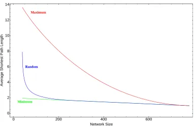
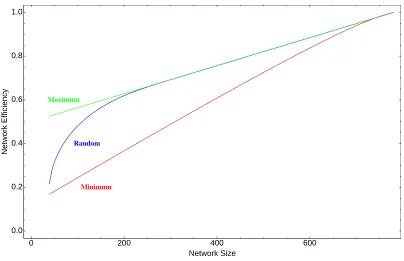
0 200 400 600 0

2 4 6 8 10 12 14

Network Size

Average

Shortest

Path

Length

Maximum

Random

[image:44.612.134.516.82.332.2]

Minimum

Figure 3.4: Tight bounds on the average distance of a graph with N = 40 vertices and 39≤m≤780 edges. These bounds have been computed analytically. The average shortest path length for random graphs has been estimated by finding the mean shortest path length of 104randomly generated graphs of the same order and size. The expected average distance of a random graph is very close to the minimum, even for relatively sparse networks. For graphs with edge density ρ >0.25, it is virtually identical to the minimum one.

the same order and size. An example that shows the tight upper and lower bounds

of the average distance of a graph with N = 40 and 39 ≤m ≤780 vertices is shown in Figure 3.4.

3.3 Betweenness Centrality

The betweenness centrality of a vertex or an edge is a measure of how important

this vertex or edge is for the communication and information propagation among the

different parts of the network. It is based on counting the number of shortest paths

among all pairs of vertices a given vertex or edge is a part of [48]. The betweenness

(45)

more generally signal propagation) among various nodes of a network, since it

indi-cates how important each vertex or edge is for the function of such a network, and

how robust it is with respect to vertex or edge removal [28]. The vertex betweenness

centrality is defined as

B(u) = ∑

(s,t)∈V2₍_G₎

s̸=u̸=t

σst(u)

σst

, (3.46)

where σst is the number of shortest paths between vertices s and t and σst(u) is the number of shortest paths between s and t that go through vertex u. Equation (3.46)

computes the total number of shortest paths of all the pairs of vertices in the graph

that go through a given vertex u. If there is more than one such path, we divide

by their total number σst, since they are assumed to be equally important. The betweenness centrality of a vertex is sometimes normalized by the total number of all

vertex pairs that we took into account for computing it, which is equal to (N₂−1).

Bnorm(u) = (_N1₋₁

2

) ∑

(s,t)∈V2(G)

s̸=u̸=t

σst(u)

σst

. (3.47)

The vertex betweenness is always nonnegative. The only vertices with betweenness

centrality equal to zero are the ones with degree equal to 1. In order to assess the

betweenness centrality of a network, we find the average of all vertices:

Bv₍_G_{) =} 1

N

∑

u∈V(G)

B(u). (3.48)

Networks with a large betweenness centrality usually have few vertices that play

a major role in the communications among every other vertex. Conversely, small

betweenness centrality indicates that the vertices of the network tend to be equally

important or that there are many different shortest paths among the various parts of

the network.

(46)

shortest paths of all vertex pairs in the network that go through a given edge:

B(f) = ∑

(s,t)∈V2₍_G₎

s̸=t

σst(f)

σst

(3.49)

where in this case σst(f) is the number of shortest paths between s and t that go through edge f. The edge betweenness centrality of the network is defined in the

same manner as before:

Be₍_G_{) =} 1

m

∑

f∈E(G)

B(f). (3.50)

The betweenness of an edge is always positive for a connected network.

The betweenness centrality of a graph is an important proxy of how robust the

network is to random vertex or edge removals. Removing a vertex or an edge with

large betweenness centrality means that the communication among many vertex pairs

will be affected, since they will now be forced to exchange information through

al-ternative, possibly longer paths. Graphs which include nodes or edges with large

betweenness centralities are sensitive to random removal of that set of vertices or

edges. The vertex or edge betweenness centrality of a graph does not give any

in-formation about the centralities of individual vertices or edges, which may largely

vary from edge to edge. For networks with the same betweenness centrality, large

variations among vertices or edges reveal a sensitivity to targeted attacks, since

re-moving the most central vertices may significantly disrupt the network function. In

this section we show that the betweenness centrality of a graph is inherently related

to its average shortest path length.

Theorem 3. The average betweenness centrality of a network G(N, m) is a linear function of its average distance,

B(G) = (N−1)( ¯D(G)−1)

Network Structure Optimization with Applications to Minimizing Variance and Crosstalk

to Minimizing Variance and Crosstalk

Dionysios Barmpoutis

Acknowledgments

Abstract

Contents

List of Figures

List of Tables

Chapter 1

Introduction

1.1

Motivation

1.2

Thesis Outline and Contributions

Chapter 2

Background and Preliminaries

2.1

Graph Theory

2.2

Wiener Processes

2.3

General Response of Linear Systems

Chapter 3

Extremal Properties of Complex

Networks

3.1

Introduction

3.2

Networks with the Minimum and Maximum

Average Distance

3.2.1

Minimum Average Distance

3.2.2

Maximum Average Distance

3.3

Betweenness Centrality