Analysis on protein structures using statistical and bioinformatical methods

(1)

2008

Analysis on protein structures using statistical and

bioinformatical methods

Aimin Yan

Iowa State University

Follow this and additional works at:

https://lib.dr.iastate.edu/rtd

Part of the

Bioinformatics Commons

, and the

Biostatistics Commons

This Dissertation is brought to you for free and open access by the Iowa State University Capstones, Theses and Dissertations at Iowa State University Digital Repository. It has been accepted for inclusion in Retrospective Theses and Dissertations by an authorized administrator of Iowa State University Digital Repository. For more information, please [email protected].

Recommended Citation

Yan, Aimin, "Analysis on protein structures using statistical and bioinformatical methods" (2008).Retrospective Theses and Dissertations. 15827.

(2)

by

Aimin Yan

A dissertation submitted to the graduate faculty

in partial fulfillment of the requirements for the degree of

DOCTOR OF PHILOSOPHY

Major: Bioinformatics and Computational Biology

Program of Study Committee: Robert L.Jernigan, Major Professor

Zhijun Wu Vasant Honavar David Fernandez-Baca

Alicia Carriquiry Kai-Ming Ho

Iowa State University

Ames, Iowa

2008

(3)

(4)

DEDICATION

I would like to dedicate this thesis to my mother(Cungui Pan), my father(Jinyuan Yan) and my

sisters(Caili Yan, Caihong Yan, Caiqin Yan, Caixia Yan) for their unconditional love. Equivalently, I

want to thank my wife, Shan Yu, for her patience and love. I also want to thank my son, Ivan Yu Yan,

(5)

LIST OF TABLES

2.1 Terminal side-chain atoms for different residue types . . . 12

2.2 Correlations between various hydrophobicity scales and Ω values for a set of

monomeric proteins and a set of dimeric proteins . . . 20

2.3 Scheff´e test for all pairwise comparisons between buried, interface, and exposed

residues . . . 23

2.4 Terminal atoms for different residue types . . . 26

2.5 The difference in Ω angle between surface regions and buried regions in protein

structures . . . 28

2.6 The difference in Ω angle between convex regions and concave regions in protein

surface . . . 29

3.1 The proteins in the training set and test set,by PDB name . . . 40

3.2 Correlation coefficients between bas, bms, bcu of backbone and side chain’s Ω

angle . . . 42

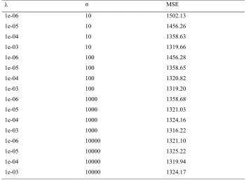
3.3 Mean square error (MSE) for the different hyperparameter settings in SVM. . . 56

3.4 Root mean square errors and correlation coefficients for angle predictions with

the training set . . . 58

3.5 Root mean square errors and correlation coefficients for angle predictions with

the test set . . . 59

3.6 Class prediction accuracy for the training set . . . 63

3.7 Class prediction accuracy for the test set . . . 63

4.1 The median structure index from the different methods for 176 NMR-derived

proteins . . . 73

4.2 Comparison for two superposition methods with the same median structure index 90

(10)

5.2 Root mean square error for the mean square fluctuations between the partial

structure and the corresponding parts in the whole complex structure in the

slowest mode . . . 101

5.3 Root mean square error for deformation energies between the partial structures

and the corresponding parts in the whole structure for the slowest mode . . . . 103

5.4 Root mean square error for the mean square fluctuations between the partial

structure and the corresponding parts in the whole structure after removing two

terminal residues in chain F for the slowest mode . . . 104

5.5 Root mean square error for the deformation energies between the partial

struc-ture and the corresponding parts in the strucstruc-ture after removing two terminal

residues in chain F for the slowest mode . . . 104

5.6 Root mean square error for mean square fluctuations between the partial

struc-ture and the corresponding parts of the complete strucstruc-ture after removing a pair

of proteins in the slowest mode . . . 106

5.7 Root mean square error for the deformation energies between the partial

struc-ture and the corresponding parts in the complete strucstruc-ture after removing a pair

of proteins for the slowest mode . . . 107

5.8 Comparison in the change of mean square fluctuations between the different

removal experiments . . . 114

(11)

LIST OF FIGURES

2.1 Definition of the angle between the center-of-mass-to-Cα_{vector and the}_Cα

-to-side-chain-atom . . . 11

2.2 Definition of the angle between the center-of-structure-to-Cα vector and the center-of-side-chain-to-Cα _{. . . .} ₁₃

2.3 Definition of three different descriptors of protein surfaces . . . 14

2.4 Average Ω values for monomeric and dimeric structures. . . 19

2.5 Ω values for buried residues and exposed residues in monomeric structures . . . 21

2.6 Ω values for buried residues, interface residues, and exposed residues in dimeric structures. . . 22

2.7 (a). Ω values for buried residues and exposed residues for small monomeric pro-teins (59−249 residues). (b). Ω values for buried residues and exposed residues for large monomeric proteins (260−907 residues). . . 25

2.8 Average Ω values for amino acid type in different solvent-accessible layers of monomeric structures. . . 27

2.9 Visualization of side chain vector in protein structure . . . 30

2.10 6-nearest-neighbor-residues-plane for each surface residue . . . 31

2.11 An example 6-nearest-neighbor-residues-plane for surface residues . . . 32

2.12 Angle correlation versus RMSD . . . 33

3.1 Definition of Ω angle . . . 42

3.2 The distribution of side chain Ω angle over secondary structures . . . 43

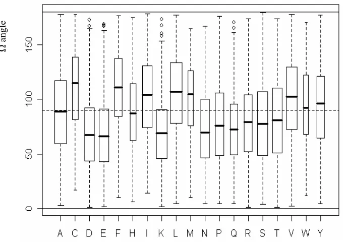
3.3 Distribution of side chain Ω angles over amino acid types . . . 43

3.4 Residual plot for linear regression model . . . 46

3.5 Relative importance of different predictors in the general linear model . . . 47

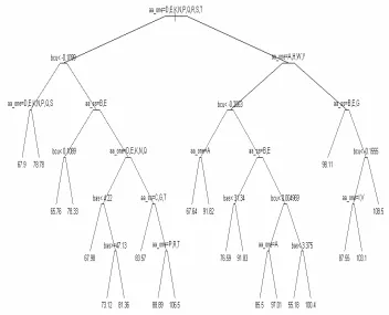
3.6 Regression tree for Ω angle prediction. . . 49

(12)

3.8 Residual plot for bagging regression tree model . . . 51

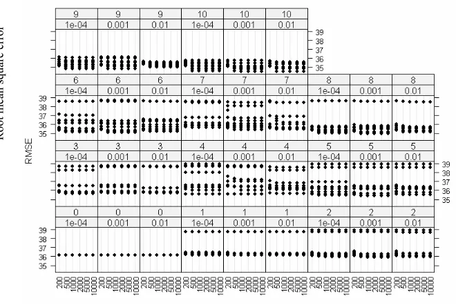
3.9 Root mean square error of training set for 1980 neural networks . . . 53

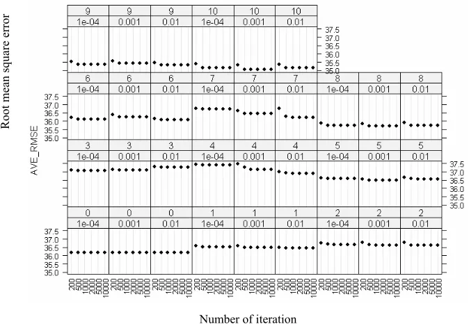
3.10 Average root mean square error of training set for 198 parameter settings. . . . 54

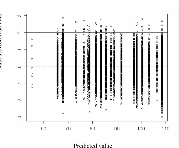
3.11 Residual plot for the neural network . . . 55

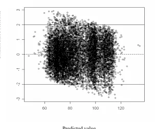
3.12 Residual plot for SVM model . . . 57

3.13 The distribution of the correlation coefficient between the random assigned side

chain Ω angle and the experimental observed Ω angle for test set(100,000 random

assignments) . . . 60

3.14 The distribution of the root mean square error between the random assigned

side chain Ω angle and the experimental observed Ω angle for test set(100,000

random assignments) . . . 61

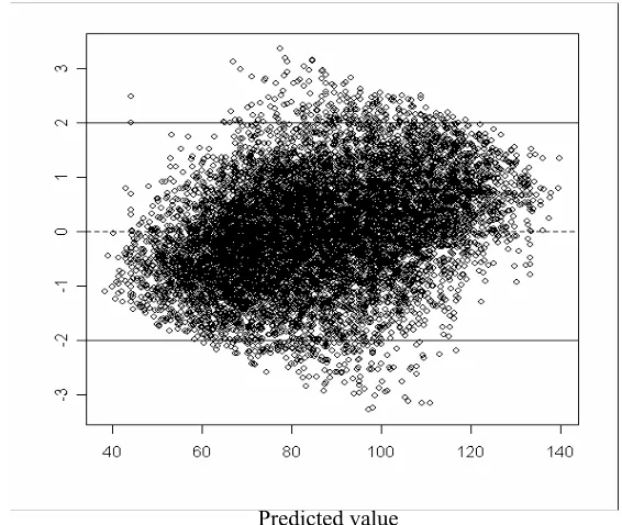
3.15 Distribution of the residuals over the different proteins in the training set. Red

line:0. Bottom blue line:-2. Top blue line:2. . . 64

4.1 The number of structures within each ensemble . . . 71

4.2 The average RMSD and its standard deviation within each ensemble . . . 72

4.3 The correlation coefficient of the mean square fluctuations using the different

median structures . . . 78

4.4 The correlation coefficient of the first principal component for the experimental

conformation changes using the two superposition methods . . . 79

4.5 The protein structures that have the larger overlap value in the least square

based method . . . 80

4.6 The source of the overlap difference for 118 proteins . . . 81

4.7 The protein structures that have the larger overlap values with the maximum

likelihood based method . . . 82

4.8 The source of the overlap difference for 58 proteins . . . 82

4.9 The cumulative overlap between the first PCs and three slowest normal modes

from ANM simulation . . . 83

4.10 The explained variance by the first 6 PCs . . . 84

4.11 The overlap between the first 6 PCs and 50 normal modes from ANM simulation 84

4.12 The distribution of RMSIP for two methods . . . 85

4.13 The distribution of RMSIP for 15,000 random orthogonal matrixs . . . 86

(13)

4.15 The overlaps between the principal components and the normal modes . . . 87

4.16 The percentage of variance explained by the principal components . . . 88

4.17 The distribution of the structures formed by the first two principal components 88 4.18 The overlap between the principal components and the normal modes . . . 89

4.19 The percentage of variance explained by the principal components . . . 89

5.1 Proteins in the 30S assembly map . . . 96

5.2 Contact map between subunits in 30S ribosome structure, using 15 ˚A as cut off distance for defining contact . . . 96

5.3 Comparison in the mean square fluctuations between the 16SrRNA part of the complete 30S structure and the single 16sRNA molecule alone . . . 99

5.4 Overlap between modes unbinding 16sRNA and modes from binding 16sRNA . 100 5.5 Root mean squares errors for the single protein removal simulations . . . 101

5.6 One protein removal experiment . . . 102

5.7 The two proteins removal experiment . . . 105

5.8 The two protein removal simulations . . . 107

5.9 The motion correlations between subunits in the 30S structure. . . 109

5.10 The motion correlations between subunits in the 30S ribosomal structure . . . . 110

5.11 The motion correlation between subunits in the 30S structure . . . 111

5.12 A simulation for removing 6 groups of protein subunits for the slowest mode . . 113

5.13 A experiment for removing 6 groups of protein subunits, respectively . . . 113

5.14 The changes for the different chains after removing the primary and the tertiary binding proteins. . . 115

5.15 The changes for the different chains after removing the secondary and the tertiary binding proteins. . . 116

5.16 The changes for the different chains after removing the tertiary binding proteins. 117 5.17 The changes for the different chains after removing the primary and the sec-ondary binding proteins. . . 118

(14)

(15)

ABSTRACT

In this PhD project, several related research topics are pursued. These projects include data mining of

coarse-grained side chain orientation in the protein data bank and the prediction of such orientation for

each individual residue using statistical learning methods, the motions of protein and protein complexes

using the elastic network model and statistical methods and clustering of structures within an ensemble

of NMR-derived protein structures.

The first research topic is about the side chain orientation in protein structures. A coarse-grained

measurement for side chain orientation is used, and the relationship between this type of side chain

orientation measurement and the hydrophobicity of residue type is established. Along with the research

on the side chain orientation, visualization software to visualize this coarse-grained side chain orientation

is developed using openGL and C++ language. In addition, several predictive models for side chain

orientation of individual residues are constructed using several statistical machine learning methods

(General linear regression, Regression tree, Bagging of regression tree, Neural Network and Support

Vector Machine).

The second topic is about the dynamics of protein and protein complexes using the elastic network

model. In this part, the effects of different superposition methods on the correspondence between the

experimental conformational changes extracted from the cluster of structures using principal component

analysis and the normal modes are studied, and we obtain a better correspondence for some protein

structures using the maximum likelihood based superposition method. In addition, we also apply the

elastic network model to study the dynamics of the small ribosomal subunit. In this project, we perform

a series of protein subunit removal computational experiments and study the effect of removing some

protein subunits on the motion of the partial 30S structures simulated with the elastic network model.

Through these studies, we find that S6 interacts with S18 in the small ribosomal subunit, which is

(16)

Another project is the application of principal component shaving method for clustering structures

in an ensemble of NMR-derived protein structures. Principal component shaving is often used to find

the similar gene expression pattern in microarray experiment, and this method is applied to cluster

similar structures in an ensemble of NMR-derived protein structures. The results show that similar

structures can be clustered together by using this method.

For this PhD project, the results from coarse-grained side chain orientation and prediction for

side chain orientation for each residue are already published. I was the first author for these two

papers. For the study of the effects of different superposition methods on the correspondence between

the experimental conformational changes from principal component analysis and the normal modes,

the application of ANM in 30S subunit and the application of the principal component shaving for

(17)

CHAPTER 1. General introduction

The first topic in this thesis concentrates on study about the coarse-grained side chain orientations

in protein structure. Generally, each protein structure is composed of 20 different types of amino acid.

The backbones of these 20 types of amino acids are the same, but their side chain groups are different.

The diversities in the properties of 20 types of amino acids come from the differences among their side

chain group, and even the atomic composition in these 20 types of side chain group are different. The

different atoms of side chain group in 20 types of amino acid are condensed to a single point using the

mathematical center of the side chain group. Under this coarse-grained level, We measured the position

of the reduced side chain group with respect to the center of protein structure using an angle between

the vector pointing from the center of all atoms in a protein structure to the specificCα atom and the

vector pointing from the reduced point of a side chain to itsCα_{atom. We found that the average angle}

value for the different amino acid types are highly related to their hydrophobicities. Similar results

were originally found by Rackovsky and Scheraga’s work in 1977 [1]. The angle they defined is an

angle between the center-of-mass-to-Cα _{vector and the}_Cα_{-to-side-chain-atom vector. The difference}

between our work and theirs is that they chose the terminal atom of each side chain as the

coarse-grained point, but we used the mathematical center as the coarse-coarse-grained point. In addition, their

results are based on a small number of monomeric protein structures only. In this thesis, the side chain

orientation measurement based on the angle we defined was studied by using three data sets. These

data sets are 144 monomeric protein structures, 192 dimeric protein structures and 1982 monomeric

protein structures. Using these data sets, the average angle values for different amino acid types were

calculated, and show that the average angle values are highly correlated with hydrophobicities of the

residue type. In addition, we further studied the difference of the average angle value for the residues

located in the different positions in protein structures; we classified residues into different categories

based on their solvent accessibilities and the convexities of their local surface, and studied the differences

of the average angle values. For dimeric proteins, the average angle value for the interface residues are

(18)

standard deviation around the average angle value is about 30-40 degree. The predictabilities of the

angle value for each individual residue are also checked by fitting several models using several statistical

machine learning methods. These statistical learning methods include the general linear regression,

regression tree and bagging, neural network, and support vector machine. The prediction accuracies

of these model are similar in qualities, but better than random assignment of side chain angle values.

Considering these characteristics of the general side chain orientation in the native structure, we also

discuss the application of the general side chain orientation on the protein tertiary prediction.

Another topic of this thesis is the study of protein motions. It is known that proteins are not static.

The polypeptide backbone and specifically the side chain move around constantly due to thermal motion

or brownian motion. Most protein structures can be determined by X-ray crystallography, but these

structures are actually the average structure from a set of protein conformations. In addition, most

biological functions require protein motion. However the experimental methods are often not sufficient

to study the motion of protein structures. Therefore computational methods have been developed to

study the motions of protein structures. Among these computational methods, molecular dynamics

simulations are the best known method. Using all-atom molecular dynamics simulations, very detailed

information about the motions of protein structures can be obtained. However the requirements of

large computer power for molecular dynamics often become a limitation for the simulation of larger

protein complexes. For this reason, the coarse-grained methods for studying motion arises. In the

coarse-grained method, the all-atom protein structure is represented by one node per residue or for

several sequential residues [2]. These coarse-grained methods are after the elastic network model which

is originally proposed by Tirion [3]. Many people use these coarse-grained elastic network models to

study the motion of protein complexs [4, 5]. Based on whether one takes the direction of motion into

account, the elastic network model used is either Gaussian network model(GNM) or anisotropic network

model(ANM). In Gaussian network model, we assume that the residues’ fluctuation about their mean

positions obey a Gaussian distribution, and all fluctuations are isotropic. The theoretical basis of GNM

comes from the polymer dynamics of Flory [6]. The elastic body is treated as a 3-dimensional mass and

spring system. The springs are assumed to follow Hooke’s law. Hooke’s law is expressed as:

− →

F =−k−→x (1.1)

Here−→F is the restoring force assigned to the material. −→x is a displacement vector for measuring distance

and movement direction with respect to the equilibrium position. k is the spring constant that indicates

the restore force per unit length of displacement vector. The negative indicates that the direction of

(19)

restore force along the displacement vector, we get the potential energy function 1.2

V =

Z

F =

Z

k∗x=1

2kx

2 _(1.2)

From equation 1.2, we can see that the potential energy is proportional to the square of the displacement

from the equilibrium position. If we extend this idea into 3-dimensional mass spring system, we can get

the following potential function:

V = (γ/2)∆RTΓ∆R (1.3)

The equation 1.3 is actually a matrix formulation for the overall potential of 3-dimensional mass spring

system. In this equation, ∆R is a fluctuation vector, and Γ is the contact matrix defined by whether

residues are closed enough to be connected with spring. This contact matrix is also called the kirchhoff

matrix, which is defined as:

Γij=

            

−1 if i6=j, Rij ≤Rc

0 if i6=j, Rij > Rc

−X

i,i6=j

Γij if i=j

            

(1.4)

In equation 1.4, Rij is the distance between the ith Cα atom and thejth Cα atom, Rc is the cutoff

distance. Based on equation 1.3, the equilibrium cross-correlations between residue fluctuations are

given by

∆Ri·∆Rj =

kBT

γ Γ

−1

ij (1.5)

Likewise, the mean square fluctuation for each residue can be calculated by:

∆R2_i =kBT

γ Γ

−1

ii (1.6)

It should be noted that the |Γ| = 0, so the inverse of Γ doesn’t exist, but there is an unique

Moore-Penrose pseudoinverse that can be used as approximation. In order to calculate the Moore-Moore-Penrose

pseudoinverse, singular value decomposition of Γ is used and this effectively remove the problematic

zero eigen values. In the anisotropic network model, we take the fact that the fluctuations are generally

anisotropic into consideration. We can derive a potential function for the ANM. This potential function

is:

(20)

In equation 1.7,H is the hessian matrix, which is defined as the following way:

H =

           

H11 H12 .. H1N

H21 H22 .. H2N

. . .. ..

HN1 HN2 .. HN N

           

(1.8)

Each element of this Hessian matrix is the second derivatives of the overall potential in equation 1.7,

It is shown in the following formula:

Hij,i6=j=      

∂2_V

∂Xi∂Xj

∂2_V

∂Xi∂Yj

∂2_V

∂Xi∂Zj

∂2_V

∂Yi∂Xj

∂2_V

∂Yi∂Yj

∂2_V

∂Yi∂Zj

∂2V ∂Zi∂Xj

∂2V ∂Zi∂Yj

∂2V ∂Zi∂Zj

     

(1.9)

Based on the equation 1.7, the equilibrium cross-correlations between residue fluctuations are given by

∆Ri·∆Rj = (kBT)Hij−1 (1.10)

The mean square fluctuation of the position of residue i can be calculated with:1.11

∆R2i = (kBT)Hii−1 (1.11)

As a coarse-grained method, GNM and ANM are already used to study the motion of proteins

extensively. Nonetheless, the simulated motion need to be validated with the experimental data. These

validation methods include the comparison between the mean square fluctuation and the experimental

crystallographic B-factors, the overlap calculation between the normal modes and the displacement

vectors between the open form and closed forms of the same protein structure. In addition, the essential

conformational changes extracted from multiple structures of the same protein using the principal

component analysis are also used to validate the normal modes generated by the elastic network model.

Usually, multiple structures are superposed by the conventional least square based method. However,

the least square based superposition method assumes the equal variance for atom fluctuations and

independence between the atoms. For some proteins, this assumption is not valid. Here, we use the

more realistic maximum likelihood based method to perform superposition, and compare the essential

conformational changes extracted from the structures using the principal component analysis and the

normal modes generated by the elastic network model for both the least squares based method and the

(21)

Besides the studies of the motion of proteins using GNM and ANM, these two methods are also

used to study the motion of protein-RNA and protein-DNA complexes. The ribosome contains protein

subunits and RNA subunits and is a macromolecule that plays the important role of protein synthesis,

so investigations of the motions of the ribosome are useful to understand the protein synthesis process.

Under the approximation of the Gaussian network and bead models, coarse-grained methods have been

used to study the motion of this type macromolecule [7, 8, 9, 10]. Yongmei Wang et al applied GNM

and ANM to study the motions of the ribosome [11], and observed some motion behaviors similar to

those observed by Tama [12]. All these results provide clear evidence for the success of elastic network

models for studying ribosome dynamics. It should be noted that all these simulation studies are based

on the intact ribosome structures including 50S and 30S subunits, and not study the influence of subunit

removal on the motion behavior of partial structures.

Ribosomes consist of two subunits, which are denoted 30S and 50S, respectively. The larger 50S

subunit contains 30 proteins(L1,L2,etc), 23SrRNA(2900 nucleotides), and 5S rRNA(120 nucleotides).

The 30S subunit includes 21 proteins(S1,S2,etc),16SrRNA(1500 nucleotides) and binds mRNA.

Ribo-some assembly is an important part of cellular processes. Some observed correlations between the rate

of ribosomal assembly and bacterial cell growth have been reported [13]. In the studies of ribosomal

assembly, the small 30S ribosomal subunit has been used as a model system. The reason for choosing

the 30S ribosomal subunit as a model system is due to its simplicity, and its assembly process can be

easily manipulatedin vitro [14, 15, 16]. Based on experimental results, the assembly map for the 30S

subunit inEscherichia coli has been determined [13]. Besides this assembly map, another map based

on the kinetics was also obtained by Powers [17]. Apart from these experimental studies of the 30S

subunit assembly, some computation methods have also been used to study 30S subunit assembly. Stagg

et al used coarse-grained Monte Carlo simulations to study the fluctuation changes upon binding the

proteins in the 3’ domain assembly to predict the contribution of the proteins for the binding site for

the sequential proteins in the S7 pathway [18]. Cui and Case also applied a coarse-grained force field in

molecular dynamics simulations to study the small subunit assembly [19]. By removing one protein or a

pair of proteins at a time from the intact 30S small subunit, Hamacher et al studied the dependencies of

protein binding to 16SrRNA for theT. thermophilus 30S small ribosomal subunit using self-consistent

pair contact probability approximation method and produced the similar dependency map of proteins

as that inE.coli established by the experimental methods [20]. Since the previous results supplied the

strong support for the application of the elastic network model for studying motion of ribosome, here

(22)

on the simulated motion of partial structures of the 30S small subunit.

The last topic of this thesis is the application of a principal component based analysis of the structure

ensemble for NMR-derived proteins. So far there are several methods for clustering the structures within

an ensemble of NMR-derived protein. These methods include pair-wise RMSD matrix based cluster

method [21] and principal component analysis based methods [22]. Principal component shaving method

is often used in miroarray data analysis to cluster similar genes [23], but it has not be used to cluster

the structures within an ensemble. We apply the principal component shaving method to cluster the

structures within the ensemble of NMR derived protein structure and show that similar structures

within an ensemble can be clustered together by using this method.

This thesis is organized as follows. In chapter 2, the coarse-grained side chain orientation metrics

are explored by using a large data set, and the relationship between this type of side chain orientation

and a residue’s hydrophobicity, residue solvent accessibility and local surface shape are studied. In

chapter 3, we develop the way to predict the angle value for each individual side chain by using several

statistical machine learning methods. In chapter 4, we study the difference in the correspondence

between the essential conformational changes and the motion generated from elastic network model

when the different superpositioning methods are applied to the same NMR-derived protein structures.

In chapter 5, we extend ANM to study the motion of the ribosome. Particularly we investigated the

influence of protein subunit removal on the simulated motions of the 30S partial structure. In chapter

6, we apply principal component shaving method to cluster the structures within an ensemble of

(23)

References

[1] S. Rackovsky and H. A. Scheraga. Hydrophobicity, hydrophilicity, and radial and orientational

distributions of residues in native proteins.Proceedings of the National Academy of Sciences of the

United States of America, 74(12):5248–5251, 1977.

[2] Doruker P., R. L. Jernigan, and I. Bahar. Dynamics of large proteins through hierarchical levels

of coarse-grained structures. J. Comput. Chem., 23:119–127, 2002.

[3] Tirion M.M. Large amplitude elastic motions in proteins from a single-parameter, atomic analysis.

Phys. Rev. Lett., 77(1905–1908), 1996.

[4] Atilgan A.R., S.R.Durell, R.L.Jernigan, M.C.Demirel, O.Keskin, and I.Bahar. Anisotropy of

fluc-tuation dynamics of proteins with an elastic network model. Biophys.J., 80:505–515, 2001.

[5] Bahar I., A.R.Atilgan, and B.Erman. Direct evaluation of thermal fluctuations in proteins using a

single-parameter harmonic potential. Fold. Des., 2:173–181, 1997.

[6] P.J. Flory. Statistical thermodynamics of random networks. Proc. Roy. Soc. Lond. A,

351(1666):351–380, 1976.

[7] Trylska J, Konecny R, Tama F, Brooks CL 3rd, and McCammon JA. Ribosome motions modulate

electrostatic properties. Biopolymers, 74(6):423–431, 2004.

[8] Chacn P, Tama F, and Wriggers W. Mega-dalton biomolecular motion captured from electron

microscopy reconstructions. J Mol Biol, 326(2):485–492, 2003.

[9] Tama F, Valle M, Frank J, and Brooks CL 3rd. Dynamic reorganization of the functionally active

ribosome explored by normal mode analysis and cryo-electron microscopy. Proc Natl Acad Sci U

S A, 100(16):9319–9323, 2003.

[10] Trylska J, Tozzini V, and McCammon JA. Exploring global motions and correlations in the

(24)

[11] Wang Y, Rader AJ, Bahar I, and Jernigan RL. Global ribosome motions revealed with elastic

network model. J Struct Biol, 147(3):302–314, 2004.

[12] Florence Tama, Mikel Valle, Joachim Frank, and III Charles L. Brooks. Dynamic reorganization of

the functionally active ribosome explored by normal mode analysis and cryo-electron microscopy.

Proc Natl Acad Sci U S A, 100(16):9319–9323, 2003.

[13] Mizushima S and Nomura M. Assembly mapping of 30s ribosomal proteins from e. coli. Nature,

226(5252):1214, 1970.

[14] Held WA, Mizushima S, and Nomura M. Reconstitution of escherichia coli 30s ribosomal subunits

from purified molecular components. J Biol Chem, 248(16):5720–5730, 1973.

[15] Held WA, Ballou B, Mizushima S, and Nomura M. Assembly mapping of 30s ribosomal proteins

from escherichia coli. further studies. J Biol Chem., 249(10):3103–3111, 1974.

[16] Culver GM and Noller HF. Efficient reconstitution of functional escherichia coli 30s ribosomal

subunits from a complete set of recombinant small subunit ribosomal proteins. RNA, 5(6):832–

843, 1999.

[17] Powers T, Daubresse G, and Noller HF. Dynamics of in vitro assembly of 16srrna into 30s ribosomal

subunits. J Mol Biol, 232(2):362–374, 1993.

[18] Stagg SM, Mears JA, and Harvey SC. A structural model for the assembly of the 30s subunit of

the ribosome. J Mol Biol, 328(1):49–61, 2003.

[19] Cui Q and Case D A. Low-resolution modeling of the ribosome assembly of the 30s subunit by

molecular dynamics simulations.Abstracts of Papers of the American Chemical Society, 229(U779–

U779), 229.

[20] Hamacher K, Trylska J, and McCammon JA. Dependency map of proteins in the small ribosomal

subunit. PLoS Comput Biol, 2(20):0080–0087, 2006.

[21] Adzhubei AA, Laughton CA, and Neidle S. An approach to protein homology modelling based on

an ensemble of nmr structures: application to the sox-5 hmg-box protein. Protein Eng, 8(7):615–

625, 1995.

[22] Howe P W. Principal components analysis of protein structure ensembles calculated using nmr

(25)

[23] Hastie T, Tibshirani R, Eisen MB, Alizadeh A, Levy R, Staudt L, Chan WC, Botstein D, and

Brown P. ’gene shaving’ as a method for identifying distinct sets of genes with similar expression

(26)

CHAPTER 2. How do side chains orient globally in protein structures?

Parts of this chapter are published in Proteins: Structure, Function, and Bioinformatics

2005,61:513-522.

Aimin Yan and Robert L. Jernigan

Abstract

An angle Ω is defined to serve as a metric for global side-chain orientations, which reflects the

orientation of the side chain relative to the radial vector from the center of the protein to an amino

acid. The side-chain orientations of buried residues exhibit characteristically different orientations than

do exposed residues, in both monomeric and dimeric structures. Overall, buried side chains point mostly

inward, whereas surface side chains tend to point outward from the surface. This difference in behavior

also correlates well with the residue hydrophobicity; so a global side-chain orientation can be viewed as a

direct structural manifestation of hydrophobicity. When various solvent-accessible layers are considered,

the behavior is relatively continuous between centrally located and exposed residues. In the case of

interfacial residues between subunits, there are statistically significant differences between exposed

residues and interface residues for ALA, ARG, ASN, ASP, GLU, HIS, LYS, THR, VAL, MET, PRO,

and overall the interface residues have an increased tendency to point inward. The local surface shape

of residues have an influence on the side-chain orientations; the side-chain orientations of residues in

concave surface regions exhibit characteristically different orientations than do residues in convex surface

regions. Presumably, these substantial differences in orientations of side chains may be a manifestation

of hydrophobic forces. Along with this research, we also develop visualization software to visualize

the general side chain orientation in protein structures. The application of these characteristics of the

general side chain orientation on protein tertiary structure prediction are also discussed.

(27)

Introduction

In protein structures, each residue type has its unique side chain group that determines the residue’s

specific behavior. Here we are interested in the average orientation of a residue’s side chain and want

to know whether side chains of residues point torward the inside of proteins or the outside of proteins

and what factors will influence the average orientation of a residue’s side chain in protein structures.

In Rackovsky and Scheraga’s early work, they defined a Θ angle to measure the average orientation of

a side chain in a protein structure. The Θ angle is an angle between the center-of-mass-to-Cα _vector

and theCα_{-to-side-chain-atom vector(see Figure 2.1),side-chain atoms are listed in Table 2.1.}

Terminal side-chain atom

Center of mass of protein

(28)

Table 2.1 Terminal side-chain atoms for different residue types

residue Side-chain atom

ALA Cβ

ARG Nη1

ASN Cγ

ASP Oδ1

CYS Sγ

GLN Cδ

GLU O1

HIS N2

ILE Cδ1

LEU Cδ1

LYS Nζ

MET C

PHE Cζ

PRO Cγ

SER Oγ

THR Cγ2

TRP Cη2

TYR Oη

VAL Cγ1

They found that there is a correlation between Θ and hydrophobicity. Nonpolar residues show a

predominance of values of Θ>90 degree and polar residues show a predominance of values of Θ<90

degree [1]. The effects of protein size on the hydrophobic behavior of amino acids measured in term

of the average reduced distances from the center of masshγi, and average side-chain orientation angle

hΘi were also studied. They found that hydrophobic behavior measured by hγi and hΘi manifests

itself more strongly in smaller proteins. For larger proteins, there is an isotropic environment in inner

sphere of radius 0.7Rgwhere no average orientational preferences of side-chain was found. Their results

also showed that the orientation preferences of Cα_-Cβ _{bonds are qualitatively similar to those of the}

side chains as a whole, indicating a strong correlation between backbone and side-chain orientations.

In Scheraga’s continuing work[2], they studied the fractions of occurrence of hydrophobic residues,

hydrophilic residues, neutral and ambivalent residues for spherical layers. They found that there is a

homogeneous region for both larger proteins and smaller proteins. Their results also indicated that the

fraction of hydrophobic residues decrease, and those of hydrophilic residues increase, gradually from the

inner to the outer layer for most proteins. They also pointed out that the proteins they studied don’t

deviate from spherical shape and the buried region of those proteins corresponds approximately to a

sphere of radiusRg around the center of mass [3]. They also defined the close surroundings of residues

(29)

local hydrophobic and hydrophilic clusters exist in protein [4].

In Yan and Jernigan’s recent publication [5], they defined another angle to measure side-chain

orien-tation(see Figure 2.2). Here−v→1 is the vector pointing from the center of all atoms in a protein structure

to a specificCα atom and−→v2 points from the center of a side chain to itsCαatom ,and Ω is the angle

between these two vectors.

Center of side-chain

Center of structure

Figure 2.2 Definition of the angle between the center-of-structure-to-Cα _vector _and _the

center-of-side-chain-to-Cα

Even with the use of a larger number of monomeric protein structures and dimeric structures, they

reached a similar conclusion as Rackovsky and Scheraga. Besides the relation between average side-chain

orientation and residue hydrophobicity, they also pointed out the relation between average side chain

orientation and the residue’s depth. Their results also showed that subunit-subunit interfacial residues

have a tendency to extend radially inward significantly, more than the usual surface residues do, which

reflects the influence of subunits association on the average side chain behaviors in dimeric structures.

By classifying the residues into different solvent accessible layers, they found that the behavior of side

chains is relatively continuous between centrally located and exposed residues. In their paper, they

emphasized that the average side chain behaviors they studied are just the global side chain behavior,

while individual cases can deviate significantly from the average behavior.

If we consider the side-chain orientations of each individual residue, this question will become highly

complicated. Since the local environment of each residue could be similar or very different. The

differ-ences in local environments could cause the differdiffer-ences in side chain orientation. The local environment

of a residue includes the position of the residue in the protein structure, its nearest neighbor residue

(30)

structure. When a residue is on the exterior of protein structure, it can be located at locations having

different protein surface shape.

So far,there are several representations of protein surfaces such as van der waals surface,

solvent-excluded and solvent-accessible surfaces. Figure 2.3 shows the definition of these types of protein

surfaces.

Figure 2.3 Definition of three different descriptors of protein surfaces

The van der Waals version considers only the atomic volumes and the size of the molecule itself

and does not take any other interacting particle(water molecules) into account. This surface definition

can’t tell us, for example, whether the small and narrow entrance of a deep cavity can be penetrated

by water molecules.

If we can determine the volume of the molecule that is not excluded for solvent molecules, then the

border of this volume would be the molecular surface that is accessible to the solvent. The general idea

behind the solution to this problem is described as follows: A solvent particle is represented by a probe,

which is a sphere of the size of the solvent. This probe is then rolled over the van der Waals surface

of the molecule. Lee and Richards[6] defined the solvent accessible surface as the trace of the center

of the solvent sphere. This is obtained by simply extending the van der Waals radii of all atoms by

the radius of the probe and assembling the surface in a similar way as the van der Waals surface. The

disadvantage is that the surface is not smooth and does not represent the real interface between the

molecule and the solvent.

A better interpretation of the probe-sphere principle is the solvent excluded surface (molecular

surface) that considers the interface between the probe and the molecule: Not the trace of the center

of the probe surface but rather the contact points between the molecule and the probe are combined

to form the surface. The surface is thus divided into contact surfaces, which is comprised of exposed

(31)

than one atom at the same time. The volume circumscribed by this surface is the real solvent excluded

volume. This kind of surface was made popular by Connollys molecular surface(MS) program [7].

The advantage of the solvent excluded surface is that it includes the benefits of the van der Waals

surfaces. Since it is based on the hard-sphere model it can be calculated quickly also for very large

systems. It is smooth which makes it possible to calculate curvatures for every point on the surface

and it is a model that provides more information than the simple 3D hard-sphere arrangement of the

van der Waals surface. Therefore the solvent excluded surfaces have not only become a valuable tool

for the calculation and prediction of certain molecular properties but also a popular representation for

the visualization of large proteins and complex systems.

As we showed in Figure 2.3, for the molecular surface of a protein, there exist many concave regions

and convex regions. Do these irregular molecular surface shapes have some influence on the average side

chain orientation of residues? In Scheraga’s paper, they pointed out that most proteins have an irregular

surface shape so that the correlations between Θ and surface location should not be exact, but they

didn’t study further the relationship between Θ and the local surface shape. Moreover in Scheraga’s

paper, they just used a small set of protein structures and did not give detailed information about the

orientation of side chains in multisubunit protein structures. In order to answer this question, we need

first to define the local shape of a molecular surface. The molecular surface shape of proteins mostly

is measured by local surface curvature. There are several methods to measure protein local surface

curvature. Connolly’s solid-angle approach is the classical method for calculating surface curvature[8].

In his method, by placing a sphere with its center on the molecular surface, the solid angle is defined by

the surface area of the sphere portion lying inside the protein divided by the sphere’s total surface area.

The second method is from differential geometry. In this method, the principal curvature of the protein

surface is calculated, the average curvature and Gaussian curvature of the surface is calculated. However

this method assumes a continuous and differential surface, which is not realistic for the real protein

surface. In order to model the real protein surface, Duncan and Olson used a Gaussian representation

of protein atoms in part to try to overcome this problem[9]. Tsodikov partitioned the non-differentiable

surface into the continuous section and then calculated the average of the curvatures of each section and

implemented two programs(FastSurf and SurfRace)[10]. The third method is called least squares-fitted

method. Cheng generated the least squares fitted sphere to a surface patch and used the radius of

sphere as the curvature measurement[11]. In his method, he transformed the sphere-fitting problem

into a solvable plane-fitting problem using a geometric transformation known as inversion. This method

(32)

differential geometry method needs in its calculation.

what is the relation between the average side chain orientation of residues and the local surface

shape? Is there some difference in average side chain orientation between residues in a concave region

and a convex region of protein surface? We could hypothesize that the average side chain orientation

in concave regions of protein surface would be more similar to the average side chain orientation inside

of a protein structure because of the greater geometric constraints on a concave surface regions and the

average side chain orientation in a convex region of protein surface might more resemble the surface

residue’s side chain behavior because of the greater freedom in convex surface regions. However we need

the exact data to support this hypothesis. Here we used Tsodikov’s program to calculate the average

curvature of molecular surface. Based on the average curvature, we identified the local surface shape

and investigated the relationship between the average side chain orientation and the local surface shape.

So far, there are many visualization software to visualize protein structure. However the software

for visualizing the general side chain orientation for all residues in a protein structure is not available.

Besides the analytical results for the general side chain orientation, we also want to visualize the general

side chain orientation. Therefore visualization software to visualize the general side chain orientation

is also developed.

Finally, the application of the general side chain orientation on the protein tertiary structure is also

discussed.

Data set and method

The used protein structures

Three set of structures are analyzed to identify the side-chain orientations of residues. The resolution

of all proteins used is better than 2.5 ˚A. These sets include 144 monomer protein structures, 192 dimer

protein structures and 1982 monomer protein structures, respectively. The set of 144 monomer protein

structures and 1982 monomer protein structures are analyzed to identify the sidechain orientations of

residues that are buried, exposed, convex regions and concave regions. The set of 192 dimeric structures

is used to study sidechain orientations that are either at subunit-subunit interfaces or exposed. All

these structures have been selected with the UniqueProt [12] program to remove sequence redundancy,

to assure that sequence identity is below 20%. Structures are extracted from the Protein Quaternary

(33)

Ω angle calculation

The Ω angle is defined as the angle between the vector pointing from residue’s Cα atom to the

geometrical center of a side chain and the vector from the geometrical center of the monomeric structure

to theCα _{atom of each residue. For any atoms having alternative positions we calculate the average}

position for each atom. We define the Ω angle over the range 0 to 180; residue side chains point radially

outward in their orientations if the Ω angle is less than 90; and if the value is greater than or equal to

90, they point inward from the center. A C++ program was written to calculate the Ω angle for the

sets of protein structures.

Residue surface area and curvature

The accessible surface areas for 144 monomer protein structure and 192 dimer protein structure are

calculated using the program NACCESS (http://wolf.bms.umist.ac.uk/naccess/). Surface residues of a

protein are defined as those residues with a relative accessible surface area>5%.

For 192 dimer protein structures, the subunit-subunit interface residues are determined by the change

in residues’ solvent accessible surface area (∆ASA). The interface residues are defined as those having

an ASA that decreases by more than 1 ˚A upon complex formation [14], and where the accessible surface

area is<= 5%. A C++ program was written to calculate ∆ ASA for each residue and to identify the

interface residues.

For the set of 1982 monomer protein structure, the residue surface areas and average curvature are

calculated by using the program surfrace 3.0 [10]. We use the Van del Waals radii of all atoms from the

set of Richards [10] and set up probe radius as 1.4 ˚A. Surface residues of a protein are defined as those

residues with a relative accessible surface area>5%. For surface residues, residues in concave region

are defined as those residues with the average curvature>= 0, residues in convex region are defined as

those residues with the average curvature<0.

Data processing and Statistical analysis

For the set of 144 monomer protein structures and 192 dimer protein structures, comparative

anal-ysis between exposed and buried residues for monomeric proteins is carried out with a nonparametric

Wilcoxon test [15]. Multiple comparisons between burial, interface and exposed groups for dimeric

proteins are made with the Scheff method [15]. We calculate P-value for these tests, and if the P-value

is below 0.05, we consider the difference to be significant; otherwise the difference is taken to be not

(34)

For the set of 1982 monomer protein structures, in order to compare the difference for surface

residues and buried residues, we calculate the average angle for surface residues and buried residues

for each residue type within each protein structures, then pair two average values for the same residue

in each protein structure, then calculate the difference for each pair within each protein structure.

Afterwards we put all the difference of same pairs of residue type together for all 1982 structures. We

did one sample t test to see if the difference in average omega value between buried residues and surface

residues for each residue is different from 0 for all 1982 structures. Since residues in concave region

and convex region of protein surface are not independent, so we calculate the average omega value for

concave region and convex region for each residue type within each protein structure. Then we calculate

the difference in the average omega value between concave region and convex region for each residue

type within each protein structure and put together all the difference for the same residue type for

1982 structures. Afterwards we did one-sample t test to see if the difference in the average omega value

between concave region and convex region for each residue type is different from 0.

Results and Discussion

Relationship between Ωangle and hydrophobicity

We calculated Ω angle for 144 monomer protein structures and 192 dimeric protein structures to

study the average side chain orientation behaviors. For the set of monomeric(144 structures) and dimeric

structures(192 structures), Ω angles are calculated for all residues in the protein structures. Figure 2.4

shows the value for both sets of structures. Overall, the correlation between the two sets is above 99

% (also see Table 2.2), which shows consistent results for both sets of structures. We compare these

Ω angle values with 47 different hydrophobicity or polarity scales (in Table 2.2), and we can see that

there are high correlations between these hydrophobicity or polarity scales and Ω angle values. From

these results, we conclude that the Ω angle is closely related to a residue’s hydrophobicity. Overall,

from the results for both monomeric structures and dimeric structures, we see that polar residue types

have a tendency for Ω values to be≥90 and the hydrophobic residues have a tendency for Ω values to

(35)

(36)

(37)

Difference in Ωangle between exposed and buried residues in 144 monomeric structures

A residue’s solvent accessibility is well known to be related to its hydrophobicity. The results

above show that the Ω angle is also related to residue hydrophobicity, so we want to investigate what

the difference in Ω angle is, between exposed and buried residues in monomeric structures. From

Figure 2.5, we can see that the Ω angles of buried residues and exposed residues are quite different for

most residues except CYS. A Wilcoxon test shows these differences to be statistically significant. For

CYS, the average Ω angles for exposed and buried residues are not different, which could be a reflection

of the constraining influence of the disulfide bonds of these residues.

Figure 2.5 Ω values for buried residues and exposed residues in monomeric structures

Black: exposed residues White: buried residues

Difference in Ω angle distributions between exposed, interfacial, and buried residues in 192 dimeric Structures

To learn what the differences in Ω angles are between exposed, interfacial, and buried residues in

dimeric structure, we calculate the average Ω angles for residues in these different categories. As we

have seen in monomeric structures, average Ω angle values for buried residues and exposed residues are

statistically different except for CYS. In Figure 2.6, it can be seen that for exposed residues and

inter-facial residues, these are statistically significantly difference between interinter-facial residues and exposed

residues in their average values of Ω for ALA, ARG, ASN, ASP, GLU, HIS, LYS, THR, VAL, MET,

and PRO. However, the differences are not statistically significant for CYS, GLN, ILE, LEU, PHE,

SER, TRP, and TYR (p-values are>0.05 for these residues types in Table 2.3). So we observe that for

(38)

significantly, more than the usual surface residues do, evidently corresponding to residue reorientations

to accommodate binding partners, and a behavior more similar to buried residues in general.

Figure 2.6 Ω values for buried residues, interface residues, and exposed residues in dimeric structures.

(39)

Table 2.3 Scheff´e test for all pairwise comparisons between buried, interface, and exposed residues

B, buried residues; I, interfacial residues; E, exposed residues P, polar residue; H, hydrophobic residue

p-Values≤0.05 are taken to be significant

In Figure 2.5, the average angle and variance for 19 types of exposed amino acids are 97±11, the

average angle and variance for 19 types of buried amino acid type are 76±6. In Figure 2.6, the average

angle and variance for 19 exposed amino acid type are 97±11, the average angle and variance for 19

buried amino acid type are 76±6, the average angle and variance for 19 types of interface amino acid

type are 89±7. These results show there is a greater variance in the angles of the exposed residues,

while the angles of the buried and interface residues exhibit less variance, and that interface residues

behave overall in an intermediate way. So the differences in the angles of the exposed residues may

(40)

Relationship between Ωangle and mean residue depth

Pintar et al [16] reported that mean residue depths correlate well with hydrophobicity based on 136

nonhomologous, monomeric crystal structures and they calculated mean residue depths for each of the

20 amino acid types. Because our results show that the Ω angle is also related to residue hydrophobicity,

we want to know what the relationship is between the Ω distribution and the mean residue depth. We

calculate correlation coefficients between Pintar’s residue depths and our Ω angle (from Table 2.2), and

find that there is a 95% correlation between Ω angle value and mean residue depth for both monomeric

structures and dimeric structures. This means that the greater the residue’s depth, the more inward

the sidechain points. Pintar indicated that mean residue depth can serve as a good structure-based

index for hydrophobicity. Here we likewise find that Ω angles similarly follow this effect. Moreover,

no assumption has been made here regarding the physicochemical properties of each amino acid in the

calculation of the Ω angle, so our Ω values are fully unbiased and fully empirical in nature.

Ω angle for different sizes of monomeric protein structures

We have already shown that there is a predominance of Ω angles>90 for exposed residues. We want

to know whether the protein size has any influence on this behavior. We divided 144 monomeric protein

structures into two sets(a small size set of protein structures with 93 structures ranging from 59−249

residues, and a large size set of protein structures with 51 structures having from 260−907 residues).

Then we calculate the Ω angle values for exposed residues and buried residues for these two sets. Figure

2.7(a) and (b) shows the values for both sets of structures. From Figure 2.7(a) and (b), we can see that

there is a predominance of Ω angles that are>90 for exposed residues and a predominance of Ω angles

below 90 for buried residues for both sets, and if we compare the Ω angle values of exposed residues

between the small size proteins and the large size proteins, we find the Ω angle values for exposed

residues of small size protein structures to be larger than those of large protein structures for almost all

types of amino acids. To the contrary, for the buried residues, usually Ω is smaller for small proteins,

(41)

Figure 2.7 (a). Ω values for buried residues and exposed residues for small monomeric proteins (59−249 residues). (b). Ω values for buried residues and exposed residues for large monomeric proteins

(260−907 residues).

Black: exposed residues. White: buried residues.

Variation of Ω angle in different solvent-accessible layers of structure

To learn about the behavior of the Ω angle values for different solvent-accessible layers of monomeric

structures, we divided residues into different layers based on solvent accessible areas. Figure 2.8 shows

the results for all residue types. As we showed above, when the residues become more solvent accessible,

the Ω angles increase universally, and here we see almost monotonic behavior. We use terminal atoms

of each residue in our calculations(about terminal atom for each residue type, see table 2.4), and when

(42)

Table 2.4 Terminal atoms for different residue types

residue Side-chain atom

ALA CB

ARG CZ

ASN CG

ASP CG

CYS SG

GLN CD

GLU CD

HIS CG

ILE CD1

LEU CG

LYS N Z

MET CE

PHE CZ

PRO CG

SER OG

THR CB

TRP CH2

TYR OH

VAL CB

However, we can see from Figure 2.8(a), for LEU and MET, that the average Ω angles decrease

in some layers of monomeric structures although the average Ω angles for these two types of residues

increase globally as residues become more solvent accessible. For some other types of residues, we find

similar results (Fig 2.8). Particularly for Trp, the non-monotonic variation of the Ω angle is significant.

Because the number of Trp residues in these structures is relatively small in comparison with other

amino acids, we believe that this behavior for Trp may originate in part from statistical errors because

(43)

(a) (b)

(c)

Figure 2.8 Average Ω values for amino acid type in different solvent-accessible layers of monomeric

struc-tures.

Cen: the geometrical centers of side chains. Ter: the terminal atoms of residues.

The difference of side chain orientation preference in surface regions and buried regions in 1982 monomeric protein structures

Since 144 monomeric protein structures and 192 dimeric protein structures are not sufficiently large

(44)

We use 1982 monomeric structures in our studies. For each protein structure, we classify the residues

into buried residues and exposed residues based on the accessibility of residue to water. Then we

calculate the average Ω value for buried residues and exposed residues, respectively. Afterwards we

calculate the difference between these two average Ω values for each residue type within one protein

structure. we performed this procedure for 1982 protein structures, then we perform a one sample t

test to see whether these differences are statistically significant different from 0. We also calculate the

95% confidence interval for this difference. These results are in Table 2.5.

Table 2.5 The difference in Ω angle between surface regions and buried regions in protein structures

residue 95% CI low bound 95%CI upper bound mu p-value

ALA 21.51 23.58 22.54 ***

ARG 24.72 29.97 27.35 ***

ASN 21.32 25.07 23.19 ***

ASP 20.05 23.63 21.84 ***

CYS -0.07 4.77 2.35 0.0575

GLN 26.40 31.24 28.82 ***

GLU 26.22 30.84 28.93 ***

HIS 19.18 23.91 21.54 ***

ILE 12.56 15.14 13.85 ***

LEU 14.74 16.69 15.72 ***

LYS 34.89 41.85 38.37 ***

MET 15.97 20.12 18.05 ***

PHE 9.73 12.46 11.09 ***

PRO 19.21 22.56 20.89 ***

SER 19.57 22.35 20.96 ***

THR 24.10 26.95 25.52 ***

TRP 9.67 14.75 12.21 ***

TYR 16.98 20.33 18.65 ***

VAL 14.01 16.33 15.17 ***

Table 2.5 shows that the 95% confidence interval for most of residue types except CYS does not

include 0 andp-values are less than 0.05, which means that the differences in Ω angle between exposed

residue and buried residues except CYS are statistically significant. Since we obtain this difference by

subtracting the average Ω angle values for buried residues from the average Ω angle values for exposed

residues. The differences for all residue types are greater than 0. So it can be seen that the exposed

residues have larger Ω angles, which mean they point more outward. However the buried residues have

(45)

The influence of the local surface shape on the side chain orientation preference

From comparison between surface residues and buried residues for the 1982 monomeric protein

structures, we know that the surface residues tend to point outward globally, but we still see some large

variations in Ω angle for residues on protein surfaces. We anticipate that there are some other factors

that have some influence on the orientation of side chain for residues on the protein surface. Next we

identify the local surface shape and study its influence on the orientation of side chains. We classify the

surface residues into residues in concave regions and residues in convex regions based on the average

surface curvature. We calculate the average Ω angle value for residues in concave region and residues in

convex region and get the difference in Ω angle for residues between these two regions, then we perform

one sample t test to see if there is a statistically significant difference between residues in concave regions

and convex regions. These results are shown in Table 2.6. Table 2.6 shows that the 95% confidence

interval for all residue types does not include 0 and thatp-values are below 0.05, which means that the

differences in Ω angle between residues in convex region and residues in concave region are statistically

significant. We obtained this difference by subtracting the average Ω angle value for residues in concave

regions from the average Ω angle value for resdiues in convex regions. The differences for all residue

types are greater than 0. So it can be seen that the residues in convex regions have large Ω angles,

which means they tend to point outward. However the residues in concave regions have small Ω angles,

which means they tend to point inward.

Table 2.6 The difference in Ω angle between convex regions and concave regions in protein surface

residue 95% CI low bound 95%CI upper bound mu p-value

ALA 25.87 28.31 27.09 ***

ARG 16.77 19.08 17.92 ***

ASN 17.07 19.71 18.39 ***

ASP 12.36 14.58 13.47 ***

CYS 12.74 21.17 16.96 ***

GLN 17.21 19.95 18.58 ***

GLU 15.77 17.79 16.78 ***

HIS 17.03 20.47 18.75 ***

ILE 23.93 27.26 25.59 ***

LEU 23.96 26.54 25.25 ***

LYS 16.20 18.58 17.39 ***

MET 21.57 26.94 24.26 ***

PHE 23.39 27.32 25.36 ***

PRO 18.44 21.23 19.84 ***

SER 18.49 20.96 19.72 ***

THR 18.58 21.16 19.87 ***

TRP 17.07 23.32 20.19 ***

TYR 18.65 21.84 20.25 ***

Analysis on protein structures using statistical and bioinformatical methods

2008