Dynamic Earthquake Source Modeling and the Study of Slab Effects

(1)

Thesis by

Kangchen Bai

In Partial Fulfillment of the Requirements for the

Degree of

Ph.D. of Geophysics and Seismology

CALIFORNIA INSTITUTE OF TECHNOLOGY

Pasadena, California

2019

(2)

Kangchen Bai

ORCID: 0000-0002-9788-6404

(3)

First of all, I would like to thank my research advisors without whose support this

work would never have been possible. Prof. Jean-Paul Ampuero introduced me

to the topics of dynamic rupture and earthquake cycle simulation which greatly

practiced analytical skills and opened my eye to the area of super computing. His deep understanding of those topics and his brilliant physics intuition enabled us to

pierce through the complications and grasp the underlying simplicity. Prof. Don

Helmberger introduced me to global seismology. His great enthusiasm and passion

on seismograms really inspired me towards making discoveries from waveforms.

He also has masterful skills in modeling which I hope that I could have learned

more.

I thank my past and present advisory committee: Rob Clayton, Jean-Philippe Avouac and Jennifer Jackson and my minor program advisor Thomas Hou for their helpful

advises on course development and guidance at every critical stage of my doctoral

study. My attitude goes to Victor Tsai for providing me the experience as a teaching

assistant that greatly improve my skills to communicate abstract concepts and make

rigorous explanation. I also thank Jean-Philippe Avouac and Zhongwen Zhan

for fruitful discussions I had with them on my research projects. I thank Mike

Gurnis, Mark Simons, Nadia Lapusta, Joanna Stock for teaching me Geodynamics,

Geodesy, Fracture dynamics and Plate tectonics which completes my knowledge in

other apsects of Geophysics.

I am grateful to a lot of former seismolab students and postdocs: Daoyuan Sun,

Shengji Wei, Han Yue, Dunzhu Li, Yiran Ma, Asaf Inbal, Yingdi Luo, Yihe Huang,

Daniel Bowden and Vish Ratnaswamy for their helpful advices on my research and

career development. I thank my office mates: Yiran Ma, Semechah Lui, Voonhui

Lai, Jorge Castillo, Zhichao Shen and Valere Lambert for a lot of fun chats and

discussions. I am fortunate to have Xiaolin Mao as my classmate, together with

whom we overcame a lot of difficulties and challenges. I thank my friends who

are also pursuing Ph.D.s all around the globe: Xiaopeng Bian, Qingyuan Yang and Hongyu Zeng for their companion during the highs and lows.

I thank Priscilla Mclean, Sarah Gordon, Donna Mireles, Kim Baker-Gatchalian,

Rosemary Miller, Michael Black and Naveed Near-Ansari for caring about

(4)

I am deeply indebted to Xiaodong Song, Mingjie Xu and Ning Mi who are my

geo-physics teachers at Nanjing university for introducing me to the area of geogeo-physics.

My attitude also goes to my mentors in Schlumberger Houston namely, James Xu,

Kun Jiao, Xing Cheng, Dong sun and Denes Vigh, with whom I spent two summers

doing an intership. Our seamless collaborations led to considerable progress towards

new imaging techniques during which I learned a lot of valuable knowledge about

seismic imaging and industrial programming.

Finally, I would like to thank my family, my father and mother, my grandmother and my uncle Ben for their unconditional love and support 10,000 km away across the

(5)

In this Thesis, I report my Ph.D. research on two major issues that are devoted towards

constructing more realistic earthquake source model using computational tools: (1)

constructing physically consistent dynamic rupture models that include complexities

in fault geometry as well as heterogeneous stress and frictional properties inferred from observations; (2) study the effect of subducting slab structure on earthquakes

that occur inside it with a special focus on the teleseismic waveforms.

Fault step over is one of the most important geometric complexities that control the

propagation and arrest of earthquake ruptures. In Chapter 2, we study the role of

seismogenic depth and background stress on physical limits of earthquake rupture

across fault step overs. We conclude that the maximum step over distance that

a rupture can jump is approximately proportional to seismogenic depth. We also conclude that the pre-stress conditions have a fundamental effect on step over jump

distance while the critical nucleation size has a secondary effect.

Seismic wave carries information of source as well as structures along the path it

travels. It was found that seismic waves generated by shallow events in subduction

zones whose ray path coincide with the down going slab structure display waveform

complexities that feature multipathing. In Chapter 3, we study deep earthquakes

whose depth phases sample the slab structure on their way up to the surface.

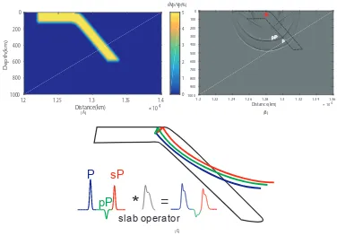
Dif-ferential travel time sP-P analysis shows a systematic decrease of up to 5 seconds from Europe to Australia and then to Pacific which is indicative of a dipping high

velocity layer above the source region. Finite-difference simulations showed that a

slab shaped structure that follows the Benioff zone at shallow depth and steepens

beyond 400 km produces a model that can account for the sP-P differential travel

times of 5 seconds for oceanic paths. In Chapter 4, we design a slab operator that

can be applied on the 1D synthetics to generate 2D synthetics with slab structure.

We hope this operator can be used for generating more accurate Green’s functions

that could potentially serve earthquake source inversion.

In Chapter 5, we design a dynamic rupture model of the Mw 7.8 Gorkha, Nepal

earthquake. We employ a novel approach of integrating kinematic inversion results

which provide low frequency stress distribution and stochastic high frequency stress

motivated by earthquake cycle models and observations. By doing this, we are able

(6)

concentration of high-frequency radiation in the down-dip part of the rupture.

In Chapter 6, I report my on going work on the spectral element method based

earthquake cycle simulator. Large scale earthquake cycle simulation with

consid-eration of complicated velocity structure and fault geometry is a great challenge

for numerical modeling. I tried to push forward this boundary by extending the

existing spectral element earthquake cycle simulator to enable cycle simulations

on bi-material faults. This chapter includes a benchmark test in 2D that

demon-strates the correctness of this new algorithm and an application of this method on

(7)

Bai, Kangchen and Jean-Paul Ampuero (2017). “Effect of Seismogenic Depth and Background Stress on Physical Limits of Earthquake Rupture Across Fault Step Overs”. In:Journal of Geophysical Research: Solid Earth 122.12, pp. 10, 280– 10, 298. doi:10.1002/2017jb014848. url:https://doi.org/10.1002/ 2017jb014848.

Bai and Ampuero co-designed the study. Bai conducted all the 3D dynamic rupture

(8)

LIST OF ILLUSTRATIONS

Number Page

2.1 Canonical model of two parallel, vertical strike-slip faults with a

step-over. Top: 3D view. The step-over distance is H and seismogenic

depth is W. Bottom: Side view. Nucleation is enforced on the

primary fault in a rectangular area that covers the whole seismogenic

depth. A shallow zone of negative strength drop is prescribed. . . . 8

2.2 Critical values of the ratio of strength excess to stress drop, S, that

allows ruptures to jump (a) compressional and (b) dilational step-overs with different seismogenic depthW and step-over distance H.

Each symbol is the result of a suite of simulations with fixedHandW,

but varyingSuntil the maximumSvalue required for step-over jump

is found. This critical S value is reported by colors. Two different

symbols indicate the rupture speed regime on the first fault:

sub-Rayleigh (circles) or super-shear (diamonds). Open circles are cases

in which only super-shear ruptures can jump through the step-over;

we did not determine the criticalSfor those cases. . . 12

2.3 Critical step-over distanceHcfor sub-Rayleigh ruptures as a function of seismogenic depthW and strength excess ratioSfor (a)

compres-sional and (b) dilational step-overs. The solid lines are not contours

generated from simulation data, but the contours of critical S

pre-dicted by a relation Hc/W = 0.3/S2inspired by our near-field theory and constrained by our simulation data. They serve as a visual guide

(11)

cleation sizes Lc/W (indicated by colors). Cases with sub-shear and

super-shear ruptures on the second fault are distinguished by symbols

(see legend). For compressional step-overs, the simulation results are

consistent with an inverse quadratic relation Hc/W ∝ 1/S2 at large

S > 2 and an inverse linear relationHc/W ∝ 1/S at small S < 1.5. The linear regime has two branches corresponding to sub-Rayleigh

and super-shear ruptures on the second fault. For dilational

step-overs, the results are consistent with the quadratic relation and also display sub-Rayleigh and super-shear branches. In both

compres-sional and dilational step-overs, sub-Rayleigh ruptures have larger

Hcthan super-shear ruptures at givenS. Small values ofLc/W favor super-shear. For a givenSvalue, faults with smallerLc/W can jump

wider step-overs. . . 13

2.5 Final rupture speed on the first fault as a function of the ratio between

fracture energy Gc and static energy release rateG0. Rupture speed

Vr is normalized by shear wave speedVS. The blue solid line is the

theoretical curve for 2D mode II cracks with constant rupture speed. A constant factor of 1.5 is introduced to account for 3D effects, such as curvature of the rupture front. . . 15

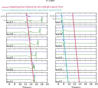
2.6 Comparison of dynamic stresses between a sub-Rayleigh rupture

(left) and a super-shear rupture (right). (a) Map view of the two

examples. Both have the same fault system geometry but different

S ratio (S = 1.27 for the sub-Rayleigh case and S = 0.64 for the super-shear case). An array of receivers (red) is placed along the

second fault near the end point of the first fault, between x = 17 km

and 27 km and at a depth of 14 km. (b) Transient shear stress τ(t) (solid green) and static strength µsσ(t)(blue) on the second fault of the sub-Rayleigh case (left) and super-shear case (right). Each panel

corresponds to a different location along the second fault (xposition

indicated by label). Stopping phases generated by sub-Rayleigh and

super-shear fronts are indicated by red and yellow lines, respectively.

The super-shear rupture did not breach the step-over because splitting

(12)

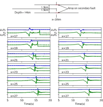
2.7 Comparison of dynamic stresses between compressional step-over

(left) and dilational step-over (right). (a) Map view of the two exam-ples. An array of receivers (red) is placed along the second fault near

the end point of the first fault, between x= 17 km and 27 km and at a

depth of 14 km. (b) Transient shear stressτ(t)(solid green) and static strengthµsσ(t)(blue) on the second fault of the compressional step-over (left) and dilational step-step-over (right). Each panel corresponds

to a different location along the second fault (x position indicated by

label). Dashed green curves are shear stresses computed in separate

simulations assuming the secondary fault remains locked. . . 18

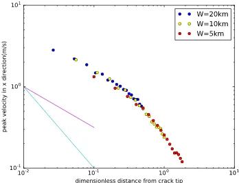
2.8 Peak ground velocity in thexdirection at 90 degree azimuth from the end of the first fault, as a function of distance to the end of the first

fault normalized by seismogenic depth. Three cases with different

seismogenic depthW are considered (see legend). . . 19

3.1 Modified from Zhan et al. (2014a). Waveform observations and

simulations for the 2009/09/10 Mw 5.9 inter-plate earthquake and the 2007/01/13 Mw 6.0 outer-rise earthquake. (A)Record-sections of observed (left panel, black) and synthetic (right panel, red)

seis-mograms for the 2009 inter-plate earthquake, aligned by the first P

arrivals. (B) Similar to (A) but for the 2007 outer-rise earthquake. (C) 2D finite-difference simulation of the 2009 inter-plate earthquake

(red star) with a high-velocity slab (outlined by the white line). The

inset shows the triangular velocity profile across the slab, with 5%

perturbation in the slab center. Black lines display the P wave ray

paths to tele-seismic distances of 30◦, 60◦and 90◦, respectively. (D)

Similar to (C) but for the 2007 outer-rise earthquake.(E) The red and

yellow stars are the interplate and outer-rise earthquakes respectively. 32

3.2 (a) PREM model with a 45° dipping slab model inserted in it. Black

and red curves are the ray path for the P and sP phases to both Eurasia (negative distances) and Pacific (positive distances). (b) Simulated

synthetic seismograms to the Pacific direction with the slab model

(13)

seismograms are color coded as red for stations in Eurasia continent

and blue for stations in the Pacific and green for stations in Australia. 35

3.4 A. CAP results of the travel time shifts between observations(black)

and synthetics(red) for P and sP phases. The lower red numbers are

the calculated double differential travel time (TsP - TP)observed-(TsP

- TP)PREM. B.The double differential travel times as a function of

distances and azimuths. C. The global map of the differential travel

time. . . 36 3.5 Comparison of synthetic predictions from the tomographic model

GyPSuM (Vs) and LLNL (Vp) given in black along with some

sam-ples of waveform data displayed in red as displayed in Figure 3.3. . . 39

3.6 We test slabs of different thickness. When the thickness of the slab

is comparable with the seismic wave length, the finite frequency

effect can be significant due to which travel time shift is very small.

But when the slab thickness is doubled in (b) the time shift become

evident. Considering our major period of 0.1s in observation, the

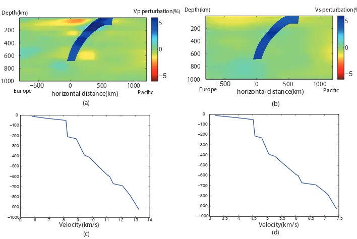
slab thickness should not be smaller than 60km. . . 39 3.7 A slab model that steepens within transition zone. We here show

the preferred model of the slab structure. Because an all 45 degree

dipping slab is not able to generate enough time shift due to the

steep take off angle of sP phase that are observed in the pacific. We

suggest that a slab model that steepens at depth can better explain the

observed travel time shift in Pacific region. (a) and (b) are the local

zoom in of the preferredVpandVs model with slab structure. (c) and

(d) are the corresponding 1D model based on which (a) and (b) are

built. . . 40 3.8 Slab model with 5% velocity perturbation that steepens at depth is

combined with tomography model. Our model is able to simulate

the differential travel time caused by slab structure but the waveform

(14)

3.9 The global P wave travel time residual compared with PREM model

estimated by CAP in frequency band 0.01−0.5 Hz for deep event (a) and shallow event (b). A deep event shows smaller travel time

devia-tion comparing with a shallow event, which may indicate complicated

subduction zone structure at shallower depth. . . 42

3.10 (A) Map view of the epicenter (yellow circle) and station distribution

for the 2013 Sea of Okhotsk Earthquake. Stations toward Pacific

and Europe are highlighted and shown in (C) and (D). (B) Vertical

velocity waveform at PASC with data in black (single station and

stacked) and the FK synthetics are shown in red (up+down), blue

(up-going) and green (down-going). Station azimuth (upper) and distance (lower) are shown at the beginning of the data. (C), (D)

show the displacement waveform of data (black) and synthetics (red)

with station names indicate at the beginning of each record. Peak

motion (in micro-meter) of data is shown at the end . . . 43

3.11 Figure 11A and 11B displays 2D cross-section along the pacific paths

sampling the slab model embedded in Lu and Grand (2016), along

with ray paths. Note the fast velocities sampled by the direct P wave.

Figure 11 C,D,E displays the differential travel times normalized to

PREM. The pP is not significantly early as suggsted for the aftershock results. . . 45

3.12 Paths towards the east Europe (A) and the west Pacific (B). The

differential travel time between depth phases and direct P shows

positive anormaly in (A) with depth phases arriving later while in (B)

the differential travel time is nearly 0. . . 46

4.1 Depth of Vs=2.5km/s in the Honshu region, the 3D velocity model is

obtained from NIED (National Research Institute for Earth Science

and Disaster Prevention). Note the 3D model stops at about 15km,

(15)

which is defined as the slip divided by the rise-time. (B) The revised

slip model based on the scheme described in Graves and Pitarka

(2010). The two circles indicate the sub-faults with their source time

function shown in (C) and (D). (C) The left panel shows the shape

of two source time functions used for the inversion (original) and for

forward calculation (rough), respectively. The length of the rough

source time function is proportional to the square root of the slip

amplitude. The right panel displays the amplitude spectra of the corresponding source time function. (D) Similar as (C), here an extra

scaling factor (0.5) is applied to determine the length of the revised

source time function (rough), thus this model has larger amplitude

spectra at high frequency bands. (E) Source time function with

flexible T1/T ratio (red) along with cosine-like source time function

(blue) . . . 52

4.3 Modified fromChu et al. (2011)0.01−0.5 Hz for deep event (a) and shallow event (b). A deep event shows smaller travel time deviation

comparing with a shallow event, which may indicate complicated subduction zone structure at shallower depth. . . 53

4.4 (A) Vs model with water layers. White star shows the position of

the sources position and triangles indicate the receivers . (B)

Ver-tical displacement for the model with water (red) and without water

(black). The waveform looks similar because the arrivals trapped in

the ocean are transmitted downward into the mantle and does not go

to the local receivers. (C) Snapshot of vertical velocity from a flat

water model (top) and a sloping water model (bottom). The source is

an explosion. The water phases are clear. A useful procedure for lo-cating off-shore earthquakes is to determine the water depth directly

above the event by modeling the various water phase arrivals, PwP

etc. Since the water depths are well known, it can help constrain the

(16)

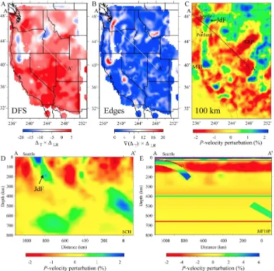
4.5 Figure modified fromChu et al. (2012). Seismic structures derived

from observed waveform complexities showing (a) dipping structure and (b) the edges of the Juan de Fuca Slab (Sun and Helmberger,

2010).(c) Map view of a tomographic image at 100km for the

west-ern United States (Schmandt and Humphreys, 2010). The location

of JdF slab derived from waveform complexity agrees with the slab

from travel-time tomography.(d) We show tomographic P wave

ve-locities of the Juan de Fuca (JdF) slab fromSchmandt and Humphreys

(2010)and (e) the hybrid model constructed from forward modeling

of waveform data and travel times. The location of the cross section

is shown as AA’ in the map. Note the difference between the color scales in Figure 2d and 2e. In Figure 2c, MTF refers to the Cape

Mendocino transform fault and SRP is the snake River Plain. . . 57

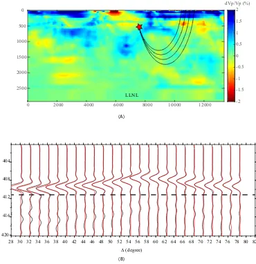
4.6 2D model and waveform comparisons. (A) 2-D cross-section of

the LLNL model from South America to the USArray. The red

star indicates the event location used in the simulation. The black

lines represent the 1-D raypaths at 50,55,60,65 degree away from the

source.(B) The waveform comparison between WKM (red) and FD

(black) using LLNL model. All traces are low-pass filtered with a

cutoff frequency of 0.4 Hz. . . 59 4.7 (A)(B) For shallow earthquakes, the ray path of the direct phases

and surface reflected phases are traveling through similar paths. So

we should assume that the slab effect on those phases to be similar.

Depending on the detailed geometric structure of the slab, when the

ray is entering or leaving the interior of the slab, multipath effect is

emphasized. We demonstrate concept of a slab operator in (C). . . . 60

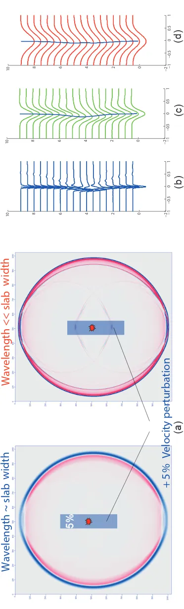
4.8 Shows the finite frequency effect of a thin high velocity slab on

seis-mic wave field.(a) is a slab model 50km wide with uniform velocity

perturbation of 5%. In (b)(c)(d) we use three sources with three different wavelengths:10km, 50km and 200km. At very high

fre-quency(b), the travel time of the slab is very clear. There are also

reflected and converted phases generated at the boundary of the slab

which can be explained by classical ray theory. When the seismic

wave length is comparable with slab width (c), the travel time effect

is blurred. At even longer wavelength, the slab structure is ignored

(17)

synthetics with that generated by convolving 1D PREM synthetics

with the slab operator. Here the wavetrain is composed of P pP and

sP phases.(b) for a source depth of 40km and (d) 80km. . . 63

5.1 Multi-cycle quasi-dynamic simulation on a rate-and-state model of

fault containing small asperities. (A) Depth dependence of friction

parameters a and b. The seismogenic zone is in the depth range

where a < b. (B) Spatial distribution of shear stress on the fault (normalized by normal stress) right before a large event that ruptures the whole seismogenic zone. (C) Top: Spatio-temporal evolution of

shear stress along a horizontal cross-section through a large asperity

shown by a long white line in (B). Bottom: temporal evolution of

slip velocity at the center of the asperity. (D) Same as (C) but for the

small asperity indicated by a short white line in (B). . . 67

5.2 Model and initial conditions for the dynamic rupture simulations.(A)

simulation region with surface topography in the middle cubic with

semi-sphere wrapped regions which is aimed to absorbing out-going

seismic wave.(B) Cross-section of the meshed mega-thrust region. The mesh is specially refined near the fault plane. (C) Small stress

patches at bottom of the seismogenic zone are superpositioned onto

the long wavelength stress field computed from kinematic rupture

model. The stress patches are randomly generated with their radius

following polynomial distribution with power -2.5. (D) Dc value in

these small patches are also stochastically perturbed downward. . . . 68

5.3 Plot of the simulations and data of vertical velocity at the strong

motion station KTP. The simulations are those of the smooth models

with different combinations of (µ_s,Dc). The blue line plots the preferred model that will be used to develop the rough model since

its pulse width and timing make a best fit to the data (magenta line). 71

5.4 Rupture time(A), rupture speed(B) and final slip distribution(C) of

the dynamic rupture simulation. . . 72

5.5 . High frequency contents 0.5-2 Hz Low frequency contents 0.05-0.2

(18)

5.6 A and B. Comparison of data, kinematic model synthetics and

dy-namic model synthetics in time dimain(A) and spectral domain(B). KTP. Vertical (C) (D) North - South (E) (F) East - West . . . 75

5.7 A. Moment rate functions generated by our smooth model (blue) and

rough model (red). B. Moment rate spectrum generated from the

smooth model (blue) and the rough model (red), and inferred from

tele-seismic data byLay et al. (2017)(yellow). . . 77

5.8 Comparison of three component high rate GPS data (black) and

synthetics generated by smooth model (red) and rough model (blue).

All the time series are filtered to a frequency band of 0.02 Hz - 0.1

Hz to get rid of the basin resonance effect. Data source : Galetzka

et al. (2015). . . 78

5.9 A: Distribution of broadband (0-3 Hz) peak ground velocity from

our rough dynamic source model. B: High-frequency peak ground

velocity (1-3 Hz). The red shaded regions are the only two districts

with a fatality rate above 1%. The yellow shaded region is the

Kathmandu city region. . . 80

5.10 Vertical ground velocity time series (A) and spectra (C) produced by

the rough dynamic source model at sites located at different distances

from the rupture as indicated by blue triangles in the map (B). Curve colors indicate their site-source distance: from blue at near-source

distances to red at farther distances. . . 81

5.11 Back projection demonstration of single frequency source (A: 0.25 Hz,

B: 2 Hz) model generated using amplitude and phase information

from the dynamic model. Due to interference of the finite source,

constructive interference at 2 Hz only occurs at the down-dip part

where source amplitude and rupture speed vary rapidly. . . 83

6.1 Sketch of the elastodynamic boundary value problem. The elastic

body is denoted as Ω while the fault plane is denoted as Γ. The quantities displacement u and stress tensor Σ can be discontinuous

across the fault plane. . . 85

6.2 Settings of the numerical simulation.(a) Boundary conditions (b) and

(c) Initial conditions. In (c), φis defined as log( Ûδ0θ/Lc) . . . 91

6.3 Comparison of slip rate atx =0 for the two methods. After 4 seismic

(19)

0.5 mm slip occurring at x= 0. . . 92

6.5 The slip profile of a bi-material fault during a full earthquake cycle.

The slip is plotted every 10 time steps with the color indicating the

maximum slip rate on the fault at that time step. . . 93

6.6 The normal stress change during a full earthquake cycle. Note that

the vertical axis is not time but the number of time steps which is not

linear with time. The white asterisk line is the plot of maximum slip

rate. The black lines cross the whole domain is the log plot of slip velocity. v1, v2 is the critical velocity for transition from dynamic

solver to quasi-static solver and the other way around. . . 94

6.7 Plot of CPU hour cost with respect to number of elements in the

domain and fitted with a power relation . . . 95

6.8 An example of a fault boundary value problem with complicated fault

geometry. . . 96

A.1 Dilational step-over jump with three nucleation attempts. Successful

nucleation in the forward direction with respect to the primary fault’s

end point. Seismogenic depth isW = 10 km. Rupture time contours on (a) primary fault and (b) secondary fault. The fault overlap section

is 0 < x < 20 km. . . 99 A.2 Nucleation in the backward direction for a dilational stepover with

W = 20 km. . . 100

A.3 The dependence of angular pattern on rupture speed Vr at different

azimuths. The dependence is smooth and weak within the range of

azimuths and speeds we are interested in. . . 102

B.1 Point source response of a single frequency source of wavelength

λ.(B) plots the response with both amplitude (blue) and phase (red) as a function of spatial location of the test sources. We assume that

the receivers have slowness from 0.3/Vp to 0.5/Vp. The solid line plot the case with receiver cover an azimuth range from 0 °to 180 °.

The dashed line plot the case with receiver cover an azimuth range

(20)

B.2 Beam forming image of three experimental line sources. The red,

blue and green solid lines are the beam forming energy (left axis) for a uniform line source , a line source with varying rupture speed and

that with varying amplitude respectively. The red dashed line are the

rupture speed and amplitude of the uniform rupture. The blue dashed

line plots the rupture speed of the line source with varying rupture

speed. The green dashed line plots the amplitude of the line source

(21)

(22)

C h a p t e r 1

INTRODUCTION

Dynamic earthquake source modeling could provide key information for prediction

of large ground motion and long term fault evolution which is very important for

hazard analysis. The foundation of dynamic earthquake source modeling was laid

by Kostrov (1964), Burridge and Halliday (1971), Madariaga (1976), and Das

and Aki (1977a) who treat the modeling problem as an elastodynamic problem

governed by elastic wave equation with a predefined discontinuous plane inside the model domain. The relative motion across this discontinuous plane is governed

by friction laws that relate the relative motion to stress (boundary traction). With

input from laboratory rock friction experiments (Brace and Byerlee, 1966; Palmer

and Rice, 1973; Dieterich, 1994)and earthquake field observations (Stuart, 1979;

Stuart and Mavko, 1979) more realistic and robust frictional models (Andrews,

1976; Ruina, 1983) have been included into the simulations. With the advance

of both modeling techniques and frictional models, researchers are able to answer

some basic questions of earthquake mechanics such as what controls the earthquake

rupture speed(Andrews, 1976; Day, 1982; Dunham, 2007) and what controls the high frequency ground motion(Madariaga, 1977; Madariaga, 1983; Madariaga et

al., 2006).

With the accumulation of earthquake observations and the fast deployment of

super-computing power during the years, numerical simulations of large earthquakes with

fine scale details are now possible. The spectral element method was introduced

into computational seismology by Komatitsch and Vilotte (1998) and was later

developed into a scalable parallel computing software package (Komatitsch and

Tromp, 2002) that can model elastic wave propagation within the real 3D earth

which further leverages the immense power of GPU computing(Komatitsch et al.,

2010). Kaneko et al. (2008) and Galvez et al. (2014) developed a dynamic fault

friction solver to couple with this elastic wave propagation software enabling large

scale rupture simulations with realistic 3D fault geometry and velocity structure.

Of those fine scale details that influence earthquake rupture propagation, step-over is

one of the most common phenomenon that feature large earthquakes. Earthquakes

(23)

In Chapter 2, I did a series of numerical simulations to probe the factors that

control the jump of step-overs for large strike slip earthquakes. In particular, special

attention is paid to one controlling factor that has not been studied extensively which

is the seismogenic zone depth. If every rupture parameter scales with seismogenic

depth, so should the critical step-over width. However, there are some dynamic

quantities that don’t necessarily scale with seismogenic depth such as the critical

nucleation size. How will that affect the scaling relation between step-over width and seismogenic depth? We addressed this issue by exploring the parameter space

spanned by these quantities i.e. finding a critical step-over distance for each plausible

parameter combination. Our work shows that the scaling relation is approximately

true for a large range of parameter combinations. While the critical nucleation size

plays a secondary role on the fundamental scaling relation.

In Chapter 5, we conduct 3D dynamic rupture simulations and some following

research on the source processes of the Mw7.8 Gorkha earthquake. By incorporating

initial static stress from finite fault inversion results and superimposing on it a stochastic stress field at the down-dip portion inspired by the earthquake cycle

simulation, we built a dynamic source model whose rupture process is spontaneously

governed by friction law. Our dynamic rupture model was able to reproduce the

earthquake source moment rate spectra and near field strong motion acceleration

spectra that fits the observed data spectra better than the kinematic finite fault model.

We also study the resolution issue of the back-projection on high frequency radiations

using tele-seismic signals. We found that the back-projection with beam-forming

technique is only able to resolve high frequency radiation from a rough rupture that

has either rapid varying rupture speed or amplitude but not a smooth rupture.

In Chapter 6, I report my recent work on the spectral element method based

earth-quake cycle simulator. I extended the work of Kaneko et al. (2011) to enable the

simulation of mode II rupture with asymmetric material properties across the fault

plane by proposing and implementing a solver for a more generalized fault boundary

value problem. I benchmarked this solver with the original work of Kaneko et al.

(2011) which confirmed the correctness of the new method. The new method can

be applied to solve the problem of bimaterial fault evolution. The Preliminary

(24)

speed and density as a function of the earth radius. The model has been widely

used in applications such as locating earthquakes. However, the oversimplified one-dimensional model may not be suitable for locating subduction zone earthquakes.

Since the subducted slab is cooler than ambient mantle, it brings in a dipping high

velocity structure into the 1D velocity structure which substantially changes the

travel time and waveform when the source is inside the slab. In Chapter 3, we study

the effect of slab structure on the depth phases, i.e. seismic wave from deep event

traveling up to the earth surface taking route inside the slab body. Our differential

travel time approach excludes the effect of velocity anomaly on the traveling path

except the segment within the slab. In Chapter 4, we develop a slab operator for

shallow events occurring inside the slab structures. Convolving 1D synthetics with this operator will generate the correct effect of the slab structure including travel

(25)

EFFECT OF SEISMOGENIC DEPTH AND BACKGROUND

STRESS ON PHYSICAL LIMITS OF EARTHQUAKE RUPTURE

ACROSS FAULT STEP-OVERS

(26)

ABSTRACT

Earthquakes can rupture geometrically complex fault systems by breaching fault

step-overs. Quantifying the likelihood of rupture jump across step-overs is important

to evaluate earthquake hazard and to understand the interactions between dynamic

rupture and fault growth processes. Here we investigate the role of seismogenic depth and background stress on physical limits of earthquake rupture across fault

step-overs. Our computational and theoretical study is focused on the canonical case of

two parallel strike-slip faults with large aspect ratio, uniform pre-stress and uniform

friction properties. We conduct a systematic set of 3D dynamic rupture simulations

in which we vary the seismogenic depth, step-over distance and initial stresses. We

find that the maximum step-over distance Hc that a rupture can jump depends on

seismogenic depthW and strength excess to stress drop ratioS, commonly used to

evaluate probable rupture velocity, as Hc ∝W/Sn, wheren =2 whenHc/W < 0.2 (or S > 1.5) and n = 1 otherwise. The critical nucleation size, largely controlled by frictional properties, has a second-order effect onHc. Rupture on the secondary

fault is mainly triggered by the stopping phase emanated from the rupture end on the

primary fault. Asymptotic analysis of the peak amplitude of stopping phases sheds

light on the mechanical origin of the relations between Hc,W and S, and leads to

the scaling regime withn=1 in far field andn=2 in near field. The results suggest

that strike-slip earthquakes on faults with large seismogenic depth or operating at

high shear stresses can jump wider step-overs than observed so far in continental

(27)

this is not always the case: ruptures can also jump across step-overs. For example,

the 2013 Mw7.7 Balochistan earthquake rupture stopped at a dilational step-over at

its southern end (Zhou et al., 2016), whereas the 1992 Mw7.3 Landers earthquake

breached four major step-overs within the Eastern California Shear Zone(Sieh et al.,

1993).

Understanding the role of step-overs on rupture propagation and arrest has both

practical and fundamental significance. An important mechanism by which

earth-quakes become large is by breaking multiple fault segments, despite the structural

barriers that separate them (Meng et al., 2012; Hamling et al., 2017; Sieh et al.,

1993). In seismic hazard analysis, the likelihood of multiple fault segments

rup-turing during a single earthquake is a crucial consideration to determine the largest expected magnitude in a complex fault system (Field et al., 2014). An important

goal is to establish quantitative relations between the efficiency of step-over jumps

and the geometrical properties of step-overs. Efforts to achieve this goal empirically

have yielded seminal results (e.g. Wesnousky, 2006; Wesnousky and Biasi, 2011;

Biasi and Wesnousky, 2016) but are ultimately limited by the small number of

earth-quakes with sufficient rupture and fault observations. Mechanical models can offer

a complementary support to such efforts, for instance by providing

mechanically-motivated functional forms to guide the development of empirical relations and

physically expected bounds to supplement empirical models.

Step-overs and other geometrical features of faults are also the subject of basic

research, especially on the relation between the short time scales of dynamic rupture

and the long time scales of fault growth. The dynamic generation of damage

and branching during earthquake rupture contributes to the long-term evolution of

fault zones (Cooke, 1997; Herbert et al., 2014; Ampuero and Mao, 2017). One

mechanism of fault growth operates by coalescence of multiple fault segments

during which the step-overs are breached(Joussineau and Aydin, 2007). If the two

neighboring fault segments interact strongly throughout their earthquake cycles, simultaneous modeling of the whole fault system is required.

Continental strike-slip earthquakes rarely manage to jump step-overs larger than

about 5 km(Wesnousky, 2006; Xu et al., 2006; Elliott et al., 2009). This has been

(28)

1999; Oglesby, 2005; Lozos et al., 2014a; Lozos et al., 2014b), even if the second

fault segment is very close to failure. A critical step-over distance Hc = 5 km has been incorporated in seismic hazard assessment models such as the The Third

Uniform California Earthquake Rupture Forecast(Field et al., 2014).

However, some recent earthquakes may have jumped step-overs much wider than

5 km. The 2010 Mw-7.2 El Mayor-Cucapah earthquake ruptured a 120 km long

multi-segment fault jumping through an apparent step-over of more than 10 km

with the possible aid of intermediary fault segments(Wei et al., 2011; Oskin et al.,

2012). During the 2012 Mw 8.6 Indian Ocean earthquake, the rupture propagated

through a complicated orthogonal conjugate fault system. In the late part of this

earthquake, back-projection rupture imaging revealed a step-over jump as wide as

20 km(Meng et al., 2012). The 2016 Mw 7.8 Kaikoura, New Zealand earthquake

made an apparent jump through a compressional step-over of 15 km(Hamling et al.,

2017) taking advantage of several linking faults which have not been previously

mapped for hazard assessment. A common feature of the latter two events is their

particularly large rupture depth extent, compared to other strike-slip events. The

Indian Ocean earthquake has a centroid depth beyond 25 km; its rupture penetrated

into the upper mantle. These observations call for a re-examination of the factors

affecting the critical over distance. Existing models of the efficiency of step-over jumps do not account for the role of key observable physical parameters, such

as the seismogenic depth, and poorly constrained frictional parameters, such as

fracture energy. With ongoing advance in earthquake data gathering and source

inversion methods, this information can be obtained and help generating a more

accurate model.

In this computational and theoretical study, we determine key physical parameters

that control the critical step-over distance in large strike-slip ruptures using numerical simulations and asymptotic analysis. We keep the model as simple as possible so that

we can use fracture mechanics arguments to gain physical insight on the numerical

modeling results.

2.2 Model

We consider two vertical, parallel strike-slip faults in a 3D homogeneous isotropic

elastic half-space, as depicted in Figure 2.1. The elastic medium has density

2700 kg/m3, P wave speed 6000 km/s and S wave speed 3464 km/s. The faults

(29)

W

slip strengthening

slip weakening

Nucleation patch

Primary fault

Secondary fault

-50 -40 -20 20

Primary fault along strike distance (km)

Nucleation patch Start of the secondary fault

0

-1

W

D

epth (k

m)

[image:29.612.120.398.79.398.2]

Negative stress drop zone

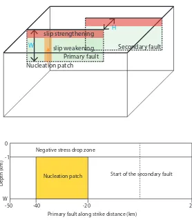
Figure 2.1: Canonical model of two parallel, vertical strike-slip faults with a step-over. Top: 3D view. The step-over distance is H and seismogenic depth is W. Bottom: Side view. Nucleation is enforced on the primary fault in a rectangular area that covers the whole seismogenic depth. A shallow zone of negative strength drop is prescribed.

two fault traces), and overlapping length D. In our simulations, L and D are

fixed while other parameters are variable. We focus on large-magnitude strike-slip

earthquakes whose rupture area have large aspect ratio L/W. The regional stress

is assumed homogeneous, resulting in a uniform normal stress of σ0 = 150 MPa

on the faults and uniform shear stress τ0 whose value is a model parameter. The

faults are governed by the linear slip-weakening friction law (Ida, 1972; Palmer

and Rice, 1973; Andrews, 1976), with uniform static and dynamic friction

(30)

Surface-induced supershear rupture(Kaneko et al., 2008)and nucleation at the free

surface on the secondary fault(Harris and Day, 1999)can substantially increaseHc for supershear ruptures (Hu et al., 2016, see also section 2.3). These two

phenom-ena have been reported in numerical simulations but not in earthquake observations.

They are thus suppressed in this study by setting a negative strength drop in the top

1 km of both faults. A linear slip-weakening friction with negative strength drop

mimics rate-and-state friction with velocity strengthening behavior whichKaneko et

al. (2008)adopted to suppress the free surface effect. Laboratory experiments

indi-cate that unconsolidated fault gouge at shallow depth exhibit velocity-strengthening

frictional properties(Marone and Scholz, 1988; Ikari et al., 2009).

Earthquake ruptures with large aspect ratio eventually turn into pulse-like ruptures

because of the no-slip constraint at the bottom of the seismogenic zone (Day,

1982; Ampuero and Mao, 2017). Their rise time is controlled by stopping phases

emanating from the lower limit of the seismogenic layer. Their rupture fronts tend

to become straight and vertical at large propagation distance. When such a vertical

rupture front suddenly changes speed, especially when it hits the vertical edge of the

fault and comes to a stop, it generates stronger coherent high-frequency radiation

than for instance a circular front (Madariaga et al., 2006). The short rise time of

a pulse-like rupture further enhances its high-frequency radiation. Hence the large aspect ratio of large ruptures exacerbates the dynamic stresses that promote

step-over jumps. However, theoretically, whenL/W is so large that the rupture becomes

a stationary pulse, the radiation strength of the stopping phase no longer depends

on rupture length (Day, 1982). Here we are interested in upper bounds on critical

step-over distance, hence we consider the limiting case of very elongated ruptures

and adopt an artificial nucleation procedure that favors straightness of the rupture

front.

To facilitate the application of our numerical model to different scales, we introduce

the following dimensionless quantities. The ratio of strength excess to stress drop,

as introduced by(Das and Aki, 1977b),

S = µsσ0−τ0

τ0−µdσ0

, (2.1)

quantifies the relative fault pre-stress level. The seismogenic depth is characterized

by the ratioW/Lc, where the length

Lc = µDc

σ0(µs− µd)

(31)

distance has been previously found to increase the critical step-over distance (Hu

et al., 2016). This can be explained by the fact that before reaching stationary

propagation, the peak slip rate of the slipping pulse keeps increasing(Day, 1982),

making the potential stopping phase stronger as fault length increases.

Ruptures are initiated by an artificial nucleation procedure intended to minimize

the curvature of the primary rupture front, which facilitates step-over jumps. We abruptly and simultaneously reduce the coefficient of friction to its dynamic value

within a vertical band extending through the full seismogenic thickness on the

primary fault . The horizontal width of this initiation band is set to 20 km in

this study by trial and error to make sure that the rupture with the largest S ratio

considered here (S = 4) can successfully nucleate on the primary fault. However,

a preferred approach to set the size of the initiation zone can be derived from the

accurate theoretical estimates developed for nucleation by over-stressed regions by

Galis et al. (2014).

The step-over geometry is characterized by the dimensionless step-over distance

H/W and overlap distance D/L. A previous study has shown a positive relation between the critical step-over distance Hc and D (Harris and Day, 1999). We fix

D/L to a large value(0.4)to ensure that the secondary fault is fully exposed to the stress change caused by the primary rupture. Our choices of values forL/Lc =140

andD/L =0.4 favor rupture across the step-over and are intended to yield an upper bound estimate ofHc/W.

Dimensional analysis of this basic problem indicates a relation between dimension-less quantities of the form

Hc/W = f(S,W/Lc) (2.3)

Here we conduct a systematic set of 3D dynamic rupture simulations to characterize

the yet unknown function f. We scan a range of values of H/W and W/Lc by

varyingWandHwhile holdingLcfixed. For each pair(H/W,W/Lc)we use binary search to find the maximumSratio(Sc)that allows the step-over to be breached.

The main focus of this study is on sub-Rayleigh ruptures (propagating slower than

Rayleigh wave speed). For super-shear ruptures (propagating faster than S wave

(32)

for a small amount of events in earthquake observations and their dynamics can

be more complicated. We nevertheless considered several super-shear cases for comparison with their sub-Rayleigh counterparts.

We use the spectral element method software SPECFEM3D(Komatitsch and Tromp,

1999). To enable this work, we extended the dynamic rupture solver implemented

by Galvez et al. (2014)to take advantage of GPU acceleration (Komatitsch et al.,

2010) which led to a decrease of 90% of the total computation time on Caltech’s

FRAM cluster. We use 5-th order spectral elements. Far from the fault we use a

coarse mesh with element size of 800 m. Within 10 km of the fault plane we refine

the mesh down to an element size of 266 m on the fault, equivalent to an average

node spacing of 66.5 m. The mesh resolves well the static process zone size≈ Lc (355 m).

2.3 Simulation results

Effects of seismogenic depthW and strength excess ratioSon critical step-over

distance

We varyWfrom 5 to 20 km with increments of 2.5 km and varyHfrom 0.5 to 3.5 km with increments of 0.5 km. This range of values covers the representative range of most strike-slip earthquakes. For each(W,H)pair, the maximumSvalue enabling step-over jumps is determined by binary search with an accuracy of 0.1 MPa. The resulting criticalScvalues for allW andHare shown in Figure 2.2.

The complete set of simulations includes both ruptures that propagated at

sub-Rayleigh speed and at super-shear speed on the first fault. For a given(W,H)pair, as S is decreased the following regimes are observed in most cases: sub-Rayleigh

rupture without step-over jump, sub-Rayleigh with jump, super-shear without jump,

and finally super-shear with jump. We then report in Figure 2.2 the two maximum

Svalues that yield a step-over jump in sub-Rayleigh ruptures (circles) and in super-shear ruptures (diamonds), respectively. There are also cases where one regime is

missing and the sequence at decreasing S is: sub-Rayleigh without jump,

super-shear without jump, and super-super-shear with jump. We did not determineScfor these

cases (open circles in Figure 2.2).

A characteristic pattern is found in the step-over jump behavior of sub-Rayleigh ruptures. The Sc values for the sub-Rayleigh cases are plotted separately in Figure

2.3, which points to a relation of the formH/W ≈ f(Sc).

(33)

Figure 2.2: Critical values of the ratio of strength excess to stress drop, S, that allows ruptures to jump (a) compressional and (b) dilational step-overs with different seismogenic depthW and step-over distanceH. Each symbol is the result of a suite of simulations with fixed H and W, but varying S until the maximum S value required for step-over jump is found. This criticalSvalue is reported by colors. Two different symbols indicate the rupture speed regime on the first fault: sub-Rayleigh (circles) or shear (diamonds). Open circles are cases in which only super-shear ruptures can jump through the step-over; we did not determine the criticalS for those cases.

(a) (b)

(34)

(a) (b)

Figure 2.4: Relation between critical step-over distance normalized by seismogenic depth, Hc/W, and strength excess S in (a) compressional and (b) dilational step-overs. Simulations span a range of normalized nucleation sizes Lc/W (indicated by colors). Cases with sub-shear and super-shear ruptures on the second fault are distinguished by symbols (see legend). For compressional step-overs, the simulation results are consistent with an inverse quadratic relationHc/W ∝1/S2at largeS > 2 and an inverse linear relationHc/W ∝1/Sat smallS < 1.5. The linear regime has two branches corresponding to sub-Rayleigh and super-shear ruptures on the second fault. For dilational step-overs, the results are consistent with the quadratic relation and also display sub-Rayleigh and super-shear branches. In both compressional and dilational step-overs, sub-Rayleigh ruptures have largerHcthan super-shear ruptures at givenS. Small values ofLc/W favor super-shear. For a givenSvalue, faults with smallerLc/W can jump wider step-overs.

function. This result can be re-interpreted as a relation between the critical

step-over distanceHcandWfor a fixedSvalue: Hc/W ≈ f(S), in which the ratioHc/W

is lower for largerS.

Further quantitative examination of the simulation results reveals the dependence of

Hc/W on Sand Lc/W. Based on the results presented in Figure 2.2 and following

the dimensional analysis leading to equation 2.3, we present in Figure 2.4 the

dependence of the ratioHc/W onSandLc/W.

In compressional step-overs, we find thatHc/Wis roughly proportional to 1/S2when

Sis large. At lowSthe sub-Rayleigh and super-shear cases are clearly separated: for a givenSvalue, sub-Rayleigh ruptures have largerHcthan super-shear ruptures. The

super-shear subset hasHc/W roughly proportional to 1/S, and the sub-shear subset

shows a hint of a similar trend at the lowestS values. The boundary between the

(35)

in dilational step-overs, for a given S value sub-Rayleigh ruptures have larger Hc

than super-shear ruptures. The simulation results at smallHc/W or largeSin both

compressional and dilational step-overs are adequately represented by the relation

Hc/W = 0.3/S2 (dashed lines in Figure 2.4). There is a slightly larger Hc/W on compressional step-overs than on dilational ones, which is consistent with previous

findings(Hu et al., 2016).

Effect of Lcon critical step-over distance and rupture speed

The ratio Lc/W modulates the relation betweenHc/W and S such that for a given

S, larger Lc/W gives smaller Hc/W (Figure 2.4). The mechanism underlying this observation is that, because the process zone scale Lc is also related to a critical

nucleation size (Uenishi and Rice, 2003; Ampuero et al., 2002), a smaller Lc/W

facilitates rupture nucleation on the secondary fault.

Apart from a nucleation effect, Lc also affects Hcby affecting the terminal rupture

speed on the primary fault. The terminal speed of sub-Rayleigh ruptures on the

primary fault depends onLc/W andS. More specifically, it depends on the ratio of

fracture energyGc = 1₂σ0(µs−µd)Dcto static energy release rateG0≈

W∆(τ0−µdσ0)

2µ ,

which is proportional to(1+S)2Lc/W. The smaller the ratioGc/G0is, the larger the

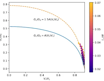
terminal rupture speed can be. In Figure 2.5 we show that the relation betweenVr

andGc/G0obtained in our simulations is consistent with the theoretical expectation

from fracture dynamics(Weng and Yang, 2017).

A more prominent effect of Lc on step-over jumps is related to its effect on

super-shear transitions. The criticalS ratio necessary for super-shear transition increases

as W/Lc increases, consistently with results of previous 3D studies (Madariaga

and Olsen, 2000; Dunham, 2007). Previous numerical simulations(Lozos et al.,

2014a; Hu et al., 2016) have shown that super-shear ruptures can breach a wider

step-over than sub-Rayleigh ruptures. In particular, when the S ratio decreases to

around 0.45, a step-over wider than 10 km can be breached by ruptures that have undergone super-shear transition assisted by free-surface effects(Hu et al., 2016).

On the contrary, in our simulations with free surface effect suppressed by a shallow

layer of negative stress drop, super-shear ruptures have shorterHcthan sub-Rayleigh

(36)

0.0

0.2

0.4

0.6

0.8 V

r

/V

s

0.0

0.1

0.2

0.3

0.4

0.5

0.6

0.7

0.8 G

c

/G

0

G

c

/G

0

= A(V

r

/V

s

)

G

c

/G

0

= 1.5A(V

r

/V

s

)

0.02

0.03

0.04

0.05

0.06

0.07 L

c

[image:36.612.128.466.100.365.2]

/W

Figure 2.5: Final rupture speed on the first fault as a function of the ratio between fracture energyGcand static energy release rateG0. Rupture speedVris normalized by shear wave speedVS. The blue solid line is the theoretical curve for 2D mode II cracks with constant rupture speed. A constant factor of 1.5 is introduced to account for 3D effects, such as curvature of the rupture front.

rupture front splits into a super-shear rupture front and a sub-Rayleigh rupture front

following the Burridge-Andrews mechanism (Andrews, 1976). These two fronts

are weaker than the original sub-Rayleigh front, hence less efficient at inducing

step-over jumps (Figure 2.6).

For most values ofH, we find two criticalSratios for step-over jump, a largerScfor

sub-Rayleigh ruptures and a smaller one for super-shear ruptures. However, there

are cases in the dilational step-overs where the step-over jump happens only when

rupture on the first fault is super-shear. In these cases, there is only one criticalS

ratio, the one corresponding to super-shear ruptures (open circles in Figure 2.2).

Effect of dynamic stresses

In principle, both static and dynamic stress transfer from the primary rupture to

(37)

stopping phase induced by supershear rupture front stopping phase induced by sub-rayleigh rupture front

x=20km 1.5km

1.5km _{Array on secondary fault}

[image:37.612.135.471.176.478.2]

Depth=-14km

(38)

by Oglesby, 2008 indicate that dynamic stresses, especially high frequency stress

peaks, are the dominant factor controlling the step-over jump behavior. He observed that the critical step-over distance depends on how sharp the initial stresses taper

at the end of the primary fault, which determines the abruptness of rupture arrest

and consequently the amplitude of stopping phases. In 3D, this effect of stopping

phases can be more complicated because the shape of the rupture front can vary

depending on S, W and nucleation processes, generating multiple high frequency

radiation phases when rupture fronts hit the boundary of the seismogenic region.

The analysis of the effect of stopping phases in 3D is made more tractable here by

forcing the rupture fronts to be straight, reaching the lateral end of the primary fault

almost simultaneously at all depths (section 2.2). As will be discussed in section 2.5, the straight rupture front assumption will generate an upper bound estimation onHc

due to the constructive interference of the stopping phases.

To demonstrate the predominance of dynamic stresses over static stresses, we show

that dynamic stresses are much larger than static stresses in our long rupture models,

in which the terminal rupture speed on the first fault is usually close to the Rayleigh

wave speed. We select a pair of compressional and dilational step-over simulations

with the following parameter settings: S = 1.27, H = 1.5 km and W = 15 km (Figure 2.7).

Static stress analysis would suggest that a dilational step-over is easier to breach

because the second fault is unclamped (subjected to normal stress reduction) by

rupture of the primary fault. However, when we consider the dynamic stresses,

results are much more complex. In the compressional step-over, static normal stress

increases in the second fault but a high frequency peak in dynamic stress brings it

to failure. In the dilational step-over example, the static normal stress on the second

fault decreases, lowering its strength and thus favoring the step-over jump, but the high frequency dynamic stress peak is not sufficient to bring the fault to failure. In

both cases, static stresses alone are not sufficient to breach the step-over, because of

their relatively small amplitude compared with dynamic stresses. A slightly larger

compressional step-over jump than a dilational one is also observed in most of the

examples presented by Hu et al., 2016 and in some of the cases in Lozos et al.

(2014a)andRyan and Oglesby (2014), especially in the sub-Rayleigh rupture cases.

This implies that the step-over distance Hc can be underestimated if only static

stress are considered, especially for a compressional step-over. Moreover, dynamic

(39)

x=20km 1.5km

[image:39.612.132.470.153.504.2]

1.5km _{Array on secondary fault} Depth=-14km

(40)

[image:40.612.123.471.94.361.2]

Figure 2.8: Peak ground velocity in thexdirection at 90 degree azimuth from the end of the first fault, as a function of distance to the end of the first fault normalized by seismogenic depth. Three cases with different seismogenic depthW are considered (see legend).

static Coulomb stresses. This pattern is determined by rupture speed and will be

discussed in section 4 and Appendix B.

2.4 Theoretical relation betweenHc/W andS

The theoretical relation between Hc/W and S cannot be derived analytically in

3D dynamic rupture problems. However, asymptotic 2D analysis provides a good

approximation to the problem. When a straight rupture front hits the lateral edge

of the seismogenic zone producing a line source of lengthW, the stopping phase

it radiates can be approximated as a cylindrical wave in the near field (0.01 < r/W < 0.1), whose amplitude decays as √1

r, and as a spherical wave in the far field(r/W > 1), decaying as 1_r (Figure 2.8). Relations between the wave amplitude in these two distance ranges, fault geometry and dynamic rupture properties are

derived in Appendix A.

(41)

thresh-observed in the simulations: Hc/W ∝ 1/S2 when Hc/W < 0.1 (near field) and Hc/W ∝ 1/SwhenHc/W > 0.2 (far field).

The previous analysis of peak dynamic stresses provides a necessary condition for

step-over jump to happen. Lozos et al. (2014a)found qualitatively in 2D simulations

an inverse relation between Hc and the critical slip weakening distance Dc which is proportional to critical nucleation size. Treating the step-over jump problem as

a static stress triggering problem, they proposed that Coulomb failure has to be

reached within an area larger than the critical nucleation size on the secondary fault

to successfully initiate rupture. Here, we further investigate the problem by analysis

of the nucleation criterion for 3D ruptures. The stopping phase of the primary

rupture induces a stress pulse traveling atSwave speed on the secondary fault. This

pulse has a large aspect ratio, it extends vertically across the whole seismogenic

depth but has a short width in the along-strike direction. Galis et al. (2017)found

that if the nucleation zone has an aspect ratio greater than 10, spontaneous runaway

rupture happens only if its shortest edge length exceeds a critical nucleation size. If

S ≤ 3, this critical nucleation size is independent of S and is equal to the critical nucleation length by Uenishi and Rice (2003), which is close to Lc. If S > 3 the nucleation condition does not depend on the aspect ratio, it is equivalent to a critical

nucleation area rather than a critical length. However, the very low initial stress

when S > 3 correspond to cases where Hc < 0.03W in our simulations. Such small step-overs are usually ignored in fault trace mapping and hazard analysis due

to the higher likelihood of connection at depth (Graymer et al., 2007) promoting

through-going rupture. Thus, for cases of interest, the critical nucleation size Lcof

Uenishi and Rice (2003)is an appropriate criterion. Therefore, increasing Lctends

to decreaseHc(Figure 2.4 color coded byLc/W). This effect is weak whenLc/Wis

small. Our previous analysis based on the maximum distance for Coulomb failure

to occur hence provides an upper bound onHc.

2.5 Discussion

Comparison to empirical observations ofHc

(42)

it is slightly modulated by the nucleation sizeLc, which is explained by the effect of

nucleation on the secondary fault by dynamic stresses carried by stopping phases.

Our modeling results are in first-order agreement with empirical estimates of

crit-ical step-over distance (Wesnousky, 2006; Wesnousky and Biasi, 2011; Biasi and

Wesnousky, 2016). The ratio of shear stress to effective normal stress on the San

Andreas fault and other major inter-plate faults has been inferred to be around 0.2 to

0.3(Noda et al., 2009), which indicates anSratio to be greater than 1.5 considering

a dynamic friction coeffcient of 0.1 and a static friction coefficient of 0.6.

When S > 1.5, our simulation results for both compressional and dilational step-overs are well represented by Hc/W ≈ 0.3/S2, and hence Hc/W < 0.2. For a typicalW = 15 km for continental strike-slip faults we expect Hc < 3 km, which agrees with previous observations (Wesnousky, 2006) and numerical simulations

(Harris and Day, 1999). The above arguments demonstrate that our new model

is consistent with the previous "5 km recipe" when applied to typical continental

inter-plate strike-slip faults.

However, our results indicate that empirical criteria for step-over jumps may not be

readily applied to faults with differentWandSunder different tectonic settings, such

as oceanic and intra-plate strike-slip earthquakes. Our theoretical results provide a

more accurate estimate ofHc for givenS andW. For a specific region, a range of

Svalues can be constrained by information on regional stresses and fault geometry.

The stress state of a fault can be estimated by projecting the regional stress tensor

onto the fault plane. The seismogenic depthW can be estimated by the termination

depth of background seismicity or by geodetic inversion of locking depth. The

nucleation size Lc is a more uncertain parameter, which may be inferred from

seismological observations of large earthquakes(Mikumo, 2003; Fukuyama, 2003), but has only a second-order effect onHc.

Additional support for the major effect of seismogenic depth on critical step-over

distance is provided by the compilation of empirical observations by Biasi and

Wesnousky (2016). Their figure 9 shows that longer ruptures with similar rupture

depth extent are not necessarily stopped by wider step-overs. This is consistent

with our theoretical arguments in which the amplitude and reach of stresses near the

(43)

variability of seismogenic thickness. The first controlling factor is the geothermal

gradient, which controls the brittle to ductile transition of the crust and the deep

seismic to aseismic transition of faults. Cooling of an old oceanic crust increases this transition depth and makes the seismogenic layer thicker, which is consistent

with a largeHcin the 2012 Indian Ocean earthquake(Meng et al., 2012). The Indian

Ocean earthquake has an extraordinary penetration depth of 50 km(Yue et al., 2012)

which is 2-3 times the depth of an average continental strike-slip earthquake. So we

expect the maximum step-over width to be around 10-15 km considering the same

Sratio. Moreover, the Indian ocean earthquake is reported to have larger stress drop

(Meng et al., 2012) indicating a smallerS ratio, which makes the observed 20 km

step-over jump (Meng et al., 2012)a possible scenario. Subduction of an oceanic

crust greatly decreases temperature around it, which may deepen the brittle-ductile transition on crustal faults in the over-riding plate. This effect has been proposed to

explain a rupture depth of 25 km in the 2016 Mw7.8 Kaikoura earthquake inferred

from geodetic data(Hamling et al., 2017). For the same thermal reason, we expect

intra-plate earthquakes to have a thicker seismogenic layer(Copley et al., 2014)and

hence a largerHc than inter-plate earthquakes.

Dynamic processes that promote large rupture width can favor wider step-over

jumps. Ruptures can penetrate deeper into the velocity strengthening region where

ruptures cannot nucleate spontaneously. Our theory actually relates the critical step-over distance to rupture width, more fundamentally than to seismogenic width.

Hence larger step-over distances are expected for large earthquake ruptures that

penetrate below the seismogenic depth, for instance due to thermal weakening

processes(Jiang and Lapusta, 2016).

Our results on strike-slip faults have implications also for other faulting types. To

apply our model to dip-slip faults, we need to replace the Mode II stress intensity

factor with the Mode III one, which involves a factor of order 1 that depends on

Poisson’s ratio. In dip-slip faults, the seismogenic width is larger, W = h/sin(α) where h is the seismogenic depth and α the dip angle. We hence expect Hc to be larger for faults with shallower dip angleα. In addition, the step-over distance conventionally defined in map-view is larger than the fault distance defined here in