promoting access to White Rose research papers
White Rose Research Online [email protected]
Universities of Leeds, Sheffield and York
http://eprints.whiterose.ac.uk/
This is an author produced version of a paper published in MATCH: Communications in Mathematical and Computer Chemistry.
White Rose Research Online URL for this paper: http://eprints.whiterose.ac.uk/77598
Published paper
Raymond, J.W and Willett, P (2003) A line graph algorithm for clustering chemical structures based on common substructural cores. MATCH:
A Line Graph Algorithm for Clustering Chemical Structures Based on
Common Substructural Cores
John W. Raymond ([email protected])
Pfizer Global Research and Development, Ann Arbor Laboratories,
2800 Plymouth Road, Ann Arbor, Michigan 48105, USA
Peter Willett ([email protected])
Krebs Institute for Biomolecular Research and Department of Information Studies, University
of Sheffield, Western Bank, Sheffield S10 2TN, UK
Abstract
There is a need among chemists for the ability to cluster large numbers of chemical
structures based on the presence of common substructural templates. This paper describes a
simple algorithm for this task that is based on a line graph interpretation of the proximity
graph and on a graph representation of 2D chemical structures. This permits the use of a
graph-theoretic similarity measure based on the maximum common edge subgraph to
determine the appropriate substructural template needed by the algorithm.
1. Introduction
The clustering of chemical structures based on pair-wise inter-molecular structural
similarities is well studied and has become an effective research tool in chemical information
management [1], with the pair-wise similarities being calculated using graph-based or
feature-based measures [2]. One of the potential limitations of the pair-wise similarity
approach, however, is that it is possible for collections of structures exhibiting a sufficient
degree of pair-wise similarity to be clustered together, but whose commonality is far less
when considered from the perspective of all of the structures in the cluster. Conversely, it is
also possible to have a collection of chemical structures which would be classified together
by a chemist based on a perceived substructural commonality but are classified into multiple
clusters by a pair-wise similarity algorithm dependent upon the variation in the
non-conserved portion of the chemical structures. What is desired is a clustering procedure that
attempts to enforce collective similarity in a cluster of chemical structures by preserving a
In this paper, we introduce a technique based on a line graph interpretation of clustering
which allows structures to be classified based on common substructural cores rather than
exclusively using a pair-wise similarity score. It is suggested that this approach may more
adequately mirror a chemist’s notion of chemical structure similarity than do existing
approaches to the calculation of structural similarity. The algorithm also allows structures
exhibiting multiple classes of activity to be assigned to multiple clusters; thereby, resolving
the problem of overlapping clusters without arbitrarily disconnecting related clusters which
can result in a loss of important information.
2. Definitions
All graphs referred to in the following text are assumed to be labeled and undirected. For
an introduction to graph related concepts and notation, the reader is referred to an
introductory text on graph theory [3]. A graph G consists of a set of vertices V(G) and a set
of edges E(G). The vertices in G are connected by an edge if there exists an edge ek = (vi,vj) ∈ E(G) connecting the vertices vi and vj in G such that vi ∈ V(G) and vj ∈ V(G). The vertex
and edge labels are denoted as w(vi) and w(vi,vk), respectively. The set of vertices adjacent to
vertex vi is the neighborhood, N(vi), of vi.
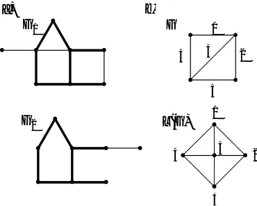
A line graph L(G) is a graph whose vertex set consists of the edge set of G; therefore, if
(vi, vj) is an edge in G it is also a vertex in L(G). A pair of vertices in L(G) are adjacent if the
two corresponding edges in G are incident on each other [4]. A maximum common edge
subgraph (MCES) is a subgraph consisting of the largest number of edges common to both
G1 and G2. Note that the MCES between two graphs is not necessarily connected or unique
by definition. To illustrate these concepts, Figure 1(a) depicts the MCES between two graphs
G1 and G2, and Figure 1(b) illustrates the line graph L(G) of graph G.
G1
G2
1
2
3 4 5
G
L(G) 1
2
3
4 5
[image:3.595.205.390.548.696.2]a) b)
3. Line Graph Formulation
As mentioned previously, the proposed clustering method addresses the question of
whether objects should be clustered together by considering information in addition to a
simple pair-wise measure of similarity. A convenient means with which to compare
graphical objects is the MCES between each pair of graphs. It has been shown that the
MCES is directly related to the edit distance between graphs [5, 6], providing a convenient
description of graph similarity. Recently, an efficient MCES algorithm for the purpose of
calculating graph similarity has been published [2, 7, 8]. In the clustering procedure
proposed here, pairs of graph objects are clustered with other pairs, based on how similar the
corresponding MCESs are to each other.
Using the terminology of Matula [9], the input to a clustering algorithm can be
represented by a proximity graph (Gp) where each vertex of the proximity graph corresponds
to an object being clustered, and an edge between any two vertices of the proximity graph is
weighted with the pair-wise similarity value between the two objects represented by the
edge’s two endpoint vertices. Rather than clustering the vertices of the proximity graph, our
algorithm clusters its edges. This is accomplished by performing the clustering on the line
graph of the proximity graph, L(Gp), rather than the proximity graph itself. Since each vertex
of L(Gp) corresponds to an edge in the proximity graph, it is weighted with the MCES
corresponding to the edge in the proximity graph. An edge of L(Gp) is weighted with the
similarity between each pair of MCESs (i.e., the MCES between two MCESs).
As an example of how the line graph approach may better identify chemical series, a data
set of 550 structures containing some well-defined series as well as numerous unrelated
compounds was clustered in two ways: using the well-known Ward’s clustering method with
the Kelley validation index [10]; and using the heuristic line graph-based algorithm proposed
in this paper. The Kelley validation index for a particular clustering at level l is calculated
using:
(
)
l kld d
d d
n
Kelley + +
− − ⋅
−
= 1
} min{ }
max{
} min{ 2
where n is the number of objects being clustered, kl is the number of clusters, dl is the
average similarity of all clusters, and min{d} and max{d} are the minimum and maximum
of dl over all clustering levels, respectively.
The 18 melatonin structures contained in the data set were all correctly clustered into a
separated the series into six different clusters. In addition, the series of 10 bioflavanoid
analogues and 5 steroid analogues were properly clustered into two distinct clusters by the
line graph method, but the Ward’s/Kelley approach clustered the bioflavanoids into three
different clusters and the steroids into two clusters. The data set also contained three distinct
opiate series: phenylpiperidines (9 compounds), phenylheptylamines (5 compounds), and
phenanthrenes (12 compounds). The proposed line graph procedure clustered the
phenylpiperidines into two clusters, the phenylheptylamines into a single cluster, and the
phenanthrenes into a single cluster. The Ward’s/Kelley method clustered the
phenylpiperidines into six clusters, the phenylheptylamines into a single cluster, and the
phenanthrenes into two clusters.
Although the proposed line graph approach to clustering may better reflect the desired
description of chemical graph similarity desired by many chemists (by focusing on how
chemicals are similar in addition to the magnitude of that similarity), any line graph-based
formulation suffers a potentially significant limitation. Since a proximity graph consisting of
N vertices can contain O(N2) edges, L(Gp) can contain O(N2) vertices and O(N4) edges, with
the result that the line graph approach can become computationally infeasible for large N.
Hence, the proposed line graph algorithm employs several simplifying heuristics in an
attempt to preserve the desirable characteristics of the line graph formulation while
significantly reducing the computational burden in practice.
4. Algorithm
The output of the proposed algorithm is “fuzzy” in the sense that an object being
clustered can appear in more than one cluster. This is a potentially desirable feature in a
clustering algorithm when dealing with possibly overlapping clusters.
The proposed algorithm is given in the following series of steps:
Step 1: Calculate Proximity Graph Similarity Values
Calculate the MCES-based similarity between each pair of chemical graphs being
clustered [2, 8] and establish a minimum similarity threshold, SGp, for which the edge
corresponding to any pair-wise similarity value not meeting the threshold value is deleted
from the proximity graph (Gp). This has the effect of significantly reducing the number of
edges in Gp (i.e., vertices in L(Gp)) and should not detrimentally affect the clustering results
as chemical structures exhibiting similar biological activity tend to exhibit similar
corresponding MCES-based similarity value if it exceeds the threshold value; otherwise, no
edge exists.
Step 2: Determine Connected Components
Next, Gp is separated into connected components (i.e., disconnected subgraphs) since
deleting edges not exceeding threshold similarity SGp may disconnect the proximity graph.
This is a simple O(N2) operation [12].
Step 3: Generate Sub-Cluster Sequences
This step is performed for each connected component of Gp. Generate a sub-cluster
sequence for each connected component by separating the neighborhood of each vertex vi in
each component using the following procedure: For each vertex vi∈V G( mp), where Gpm
denotes the mth component of the proximity graph Gp, separate the edges of the neighborhood
of vi present in the mth component, denoted Nm( )vi , into sub-clusters by calculating the
similarity between pairs of edges in m( )
i
N v and dividing the set of edges based on these
calculated similarities. The nth sub-cluster generated for the mth component will be denoted
by Cnm.
Since the similarity between each neighborhood edge is defined using the MCES between
two MCESs, the choice of similarity coefficient is important. Suppose an edge in Nm( )vi
corresponds to an MCES between two chemical graphs which are almost identical and
another edge in Nm( )vi corresponds to an MCES between one of these two chemical graphs
and a third chemical graph. The two MCESs represented by the two edges in m( )
i
N v may in
fact both contain the same substructural template characterizing the perceived
pharmacological activity, but since the MCES between the two almost identical chemical
graphs can be substantially larger than the other MCES, a similarity coefficient which
considers the size of each MCES equally may not adequately describe the desired description
of similarity between the two pairs of compounds.
To avoid this potential limitation, it is suggested that the asymmetric similarity coefficient
be used to calculate the similarity between neighborhood edges. This is
,
, ij ik / min{ ij, ik}
ij ik
S = G G G ,
where |Gij| and |Gik| are the sizes of the MCESs between the pairs of chemical graphs (Gi, Gj)
and (Gi, Gk) in the proximity graph, respectively, and |Gij,ik| is the size of the MCES between
greedy procedure if the value of Sij,ik exceeds a specified intra-cluster similarity value, Sa.
Given M connected components in the proximity graph, this process will result in M distinct
sub-cluster sequences being generated.
N N N N O O N N N N O O O O HO OH N N N N O O O N N N N O O O N N N N O O O N N N N O O
G1 G12 G2
G1 G13 G3
a) b) N N N N O O O
G12 G13
N N N N O O N N N N O O
Natom = 21
Nbond = 22
Natom = 14
Nbond = 15
Natom = 14
Nbond = 15
[image:7.595.123.470.135.598.2]G12,13
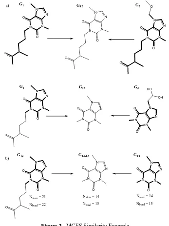
Figure 2. MCES Similarity Example
Figure 2 illustrates this scenario. First we define |G| as V(G) +
(
)
(
1− ⋅ nGp −1)
⋅E(G)⋅ α
β where |V(G)| and |E(G)| are the number of atoms and bonds in the
chemical graph, respectively. The variable n Gp represents the number of unconnected
subgraph components in graph G containing p or more edges. If all subgraphs have fewer
than p edges, then nGp will be assumed to be the total number of subgraph components. The
compatible atoms, and the constant α is a penalty score for each unconnected component
present in G. In previous studies, we have found values of p=3, α= 0.05, and β =2.0 seem
to be effective in discerning chemical similarity [2].
It can be seen in Figure 2(a) that all of the graphs (G1, G2, and G3) are related by a
xanthine substructural moiety. Both G1 and G2 are very similar, and the MCES (G12) is hence
very large. However, when G1 is compared to G3, the G13 is much smaller than G12 even
though all three chemical graphs under consideration are xanthine-based compounds.
Figure 2(b) demonstrates the comparison between MCES graphs G12 and G13. Using the
asymmetric coefficient to compute the degree of similarity based on G12,13 yields
S12,13=44/min{65,44}=1, strongly indicating that G12 and G13 should be grouped together
(indicating, indeed, that G13 is a subgraph of G12). However, using the Tanimoto coefficient
which is given as Sij,ik = Gij,ik /
(
Gij +Gik −Gij,ik)
yields S12,13 =44/(65+44−44)=0.68which is significantly lower.
Step 4: Merge Sub-Clusters
The final clustering of Gp is achieved by merging each sub-cluster sequence into full
cluster(s). In this procedure, each of the m sub-cluster sequences is considered individually.
The size of each sub-cluster, Cnm , in a particular sub-cluster sequence is determined by
summing the number of distinct vertices preserved when the edges contained in each
sub-cluster are projected onto the proximity graph (i.e., the number of unique chemical graphs
represented in each sub-cluster). The sub-clusters in each sequence are then sorted in order
of decreasing value of Cnm .
A greedy procedure is then used to merge the sub-clusters in each sequence using the
property that the current cluster and a sub-cluster are merged into a larger cluster if the
similarity value based on the number of structures in common exceeds a threshold value, Sb.
For instance, if the cluster and the sub-cluster contain 6 and 4 unique structures, respectively,
and they have 3 structures in common, then the asymmetric coefficient yields a similarity
S=3/min{6,4}=0.75. If 0.75 > Sb, then the cluster and sub-cluster would be merged into a
single cluster. The number of clusters resulting from the merging procedure will be greater
than or equal to M.
To illustrate how ordering the sub-clusters in order of non-increasing values of Cnm , a
simple test was performed on a set of 358 compounds of various activities. The threshold
being determined using the Tanimoto similarity coefficient. Two different clustering
simulations were performed. One was run using the suggested ordering of sub-clusters, and
the other was run using random selection. Each resultant clustering was then compared to a
manually constructed clustering of the same data set using the Jaccard cluster similarity
coefficient [13] which ranges from 0 to 1 with 1 indicating the two clustering are identical.
The suggested ordering resulted in a Jaccard coefficient value of 0.61, whereas, the random
selection resulted in a Jaccard value of 0.55, indicating a slight advantage for the suggested
ordering.
5. Pseudo-Code
The algorithm is given more succinctly in pseudo-code below.
Input: Set of N graphs, similarity thresholds SGp, Sa, and Sb
Output: Set of final clusters A
Procedure Line Graph Cluster() {
Generate the proximity graph (Gp) using an MCES similarity.
Prune the edges in Gp not exceeding SGp.
Separate Gp into M connected components.
Generate Sub-Cluster Sequences.
Merge Sub-Clusters into cluster subgraphs. }
Input: Set of M connected components in Gp
Output: Set of M sub-cluster sequences Cm
Procedure Generate Sub-Cluster Sequences() {
For each connected component Gmp∈Gp
{
Set n:=1.
For each vertex vi
m p
G
∈
{
Identify Nm(vi), the neighborhood of vi in m p G .
Set P:=E(Nm(vi)).
Sort the edges in P in order of non-increasing similarity.
While P≠ ∅ do {
Set Cnm:=∅.
Select the first unclustered edge ek in P.
Assign ek to sub-cluster
m n
C (i.e., Cnm:=Cnm Uek).
Remove ek from P (i.e., P:=P\ek).
While (∃ej)[ej ∈ PandSjk ≥ Sa] do
{
Select the first unclustered edge ej in P with an MCES
asymmetric similarity Sjk ≥ Sa.
Set Cnm:=Cnm Uej.
Set P:=P\ej.
}
} } } }
Input: Set of M sub-cluster sequences Cm
Output: Set of final clusters A
Procedure Merge Sub-Clusters() {
Set i:=1.
For each sub-cluster sequence Cm
{
Sort the sub-clusters Cnm of Cm in order of decreasing value of Cnm .
While Cm≠ ∅ do {
Set Ai:=∅.
Select first unclustered sub-cluster Cnm in Cm.
Assign Cnm to cluster Ai (i.e., Ai:=Ai U m n C ).
Remove Cnm from Cm (i.e., Cm:=Cm\Cnm).
While( )[ | b]
C A m m n m
n C C S S
C m
n
i ≥
∈
∃ do
{
Select the first unclustered sub-cluster Cnm in Cm|
b C A S S m n i ≥ .
Set Ai:= Ai U m n C .
Set Cm:=Cm\Cnm. } Set i:=i+1. } Set i:=i+1. } }
The algorithmic complexity of the proposed algorithm in the average case is difficult to
determine. In practice, it has been found that the MCES comparison is the time-limiting step,
and the time for clustering is dominated by the number of necessary MCES comparisons
rather than the number of clustering specific operations.
6. Conclusion
In this paper, we have addressed the clustering of chemical structures represented as
graphs based on the concept of a common substructural core using a novel line graph
approach. The technique has been presented in terms of a graph-based similarity measure
involving the MCES between two structures represented as chemical graphs although it is
equally applicable for use with a feature-based similarity method such as chemical
fingerprints where the bits in common between the two fingerprints are used in lieu of the
MCES. Since a naïve implementation of the line graph approach is computationally
similarity threshold parameters to reduce the number of comparisons necessary to form the
final clustering.
In preliminary testing of the proposed algorithm, it has been found that values of SGp, Sa
and Sb in the ranges (0.7-0.75), (0.8-0.85), and (0.6-0.7), respectively, seem to work well,
although further testing is required to establish whether the optimal values fall within these
ranges. The SGp values assume that the Tanimoto coefficient is used and that p=3, α= 0.05,
and β =2.0. The Sa range is based on the asymmetric coefficient with α equal to zero (i.e.,
no fragmentation penalty), and the Sb range is also based on the asymmetric coefficient.
Initial time comparisons indicate that the proposed algorithm is approximately 20% to
50% slower than Ward’s/Kelley clustering on data sets ranging from a few hundred to over a
thousand compounds with the time difference decreasing as the data set size increases for
MCES-based similarity calculations. The time difference is due to the sub-cluster sequence
generation procedure used in the proposed algorithm. Having described this algorithm in
detail, it now remains to compare its effectiveness for the clustering of chemical structures
when compared with existing approaches and to establish the optimal values for the threshold
parameters: this work will be reported shortly.
Aside from the proposed clustering algorithm, the line graph interpretation of clustering
introduced in this paper may prove to be useful in future clustering applications using
existing or specifically tailored algorithms.
Acknowledgments
We thank the following: Pfizer (Ann Arbor) for funding; John Blankley, Alain Calvet,
Eric Gifford, Christine Humblet, and Sherry Marcy for helpful advice and support. The
Krebs Institute for Biomolecular Research is a designated centre of the Biotechnology and
Biological Sciences Research Council.
References
1. P. Willett, Similarity and Clustering in Chemical Information Systems, Research Studies
Press, (1987).
2. J. Raymond and P. Willett, Effectiveness of Graph-Based and Fingerprint-Based
Similarity Measures for Virtual Screening of 2D Chemical Structure Databases, J.
Comput.-Aided Mol. Des., in the press.
3. R. Diestel, Graph Theory, Springer-Verlag, (2000).
4. A. van Rooij and H. Wilf, The Interchange Graph of a Finite Graph, Acta Math. Hungar.,
5. H. Bunke, On a Relation Between Graph Edit Distance and Maximum Common
Subgraph, Patt. Recog. Lett., 18 (1997), 689-694.
6. G. Chartrand, F. Saba and H. Zou, Edge Rotation and Distance Between Graphs, Cas.
Pest. Mat., 110 (1985), 87-91.
7. J. Raymond, E. Gardiner and P. Willett, Heuristics for Rapid Similarity Searching of
Chemical Graphs Using a Maximum Common Edge Subgraph Algorithm, J. Chem. Inf.
Comput. Sci., 42 (2002), 305-316.
8. J. Raymond, E. Gardiner and P. Willett, RASCAL: Calculation of Graph Similarity
Using Maximum Common Edge Subgraphs, Comput. J., in the press.
9. D.W. Matula, Graph Theoretic Techniques for Cluster Analysis Algorithms, in:
Classification and Clustering, J. Van Ryzin, Ed., Academic Press (1977), 95-129.
10. D.J. Wild and C.J. Blankley, Comparison of 2D Fingerprint Types and Hierarchy Level
Selection Methods for Structural Grouping Using Ward’s Clustering, J. Chem. Inf.
Comput. Sci., 40 (2000), 155-162.
11. M. Johnson, Relating Metrics, Lines and Variables Defined on Graphs to Problems in
Medicinal Chemistry, in: Graph Theory and Its Applications to Algorithms and Computer
Science, Y. Alavi, et al., Ed., J. Wiley & Sons (1985), 457-470.
12. E. Allburn, Graph Decomposition: Imposing Order on Chaos, Dr. Dobbs J., 16 (1991),
88,90-2,94-6,118-20,122,124.
13. G.W. Milligan, A Monte Carlo Study of Thirty Internal Criterion Measures for Cluster