Structure from Motion with Higher level Environment Representations

(1)

Structure from Motion with Higher-level

Environment Representations

Zhirui Wang

A thesis submitted for the degree of Master of Philosophy of

The Australian National University

(2)

(3)

Declaration

This thesis is an account of research undertaken between March 2016 and September 2018 at The College of Engineering & Computer Science, The Australian National University, Canberra, Australia.

Except where acknowledged in the customary manner, the material presented in this thesis is, to the best of my knowledge, original and has not been submitted in whole or part for a degree in any university.

Zhirui Wang September, 2018

(4)

(5)

Acknowledgements

This thesis is about the work I did in the last two and a half years. I really appreciate for what I have learned during the period, it is a valuable experience for studying abroad. During the journey, I learned the way about thinking in research and understand the meaning of my work. As an international student, the teaching style is far diﬀerent from my hometown but it can give the student a wider mind while also making a more creative thought. Thanks to my supervisor Laurent Kneip who guided me all the way through my research. Moreover than that, he’s personality also has a positive inﬂuence of me in life. For me, he is not only a teacher but also a good friend.

To my beloved father and mother, without whom I’ll never be able to ﬁnish my degree. Thanks to my mom Ying Xiong for her love and support. Thanks to my dad Yonghui Wang who is my guidance in life.

(6)

(7)

Abstract

Computer vision is an important area focusing on understanding, extracting and using the information from vision-based sensor. It has many applications such as vision-based 3D reconstruction, simultaneous localization and mapping(SLAM) and data-driven un-derstanding of the real world. Vision is a fundamental sensing modality in many diﬀerent ﬁelds of application.

While the traditional structure from motion mostly uses sparse point-based feature, this thesis aims to explore the possibility of using higher order feature representation. It starts with a joint work which uses straight line for feature representation and performs bundle adjustment with straight line parameterization. Then, we further try an even higher order representation where we use Bezier spline for parameterization. We start with a simple case where all contours are lying on the plane and uses Bezier splines to parametrize the curves in the background and optimize on both camera position and Bezier splines. For application, we present a complete end-to-end pipeline which produces meaningful dense 3D models from natural data of a 3D object: the target object is placed on a structured but unknown planar background that is modeled with splines. The data is captured using only a hand-held monocular camera. However, this application is limited to a planar scenario and we manage to push the parameterizations into real 3D. Following the potential of this idea, we introduce a more flexible higher-order extension of points that provide a general model for structural edges in the environment, no matter if straight or curved. Our model relies on linked Bézier curves, the geometric intuition of which proves great benefits during parameter initialization and regularization. We present the first fully automatic pipeline that is able to generate spline-based representations without any human supervision. Besides a full graphical formulation of the problem, we introduce both geometric and photometric cues as well as higher-level concepts such overall curve visibility and viewing angle restrictions to automatically manage the correspondences in the graph. Results prove that curve-based structure from motion with splines is able to outperform state-of-the-art sparse feature-based methods, as well as to model curved edges in the environment.

(8)

(9)

List of Figures

2.1 Example of a pinhole model . . . 6

2.2 Ideal relationship of the triangulation with two camera . . . 8

3.1 The system is originally designed for light-ﬁeld cameras. Here only provide a brief overview of tri-focal tensor based bootstrapping in the front-end and the representation of lines and line-based bundle adjustment in the back-end 11 3.2 Multiple-view geometry of 3D line observations. . . 13

3.3 The lightﬁeld camera used in this project . . . 15

3.4 Example 3D lines reconstructed by our light-field SLAM pipeline on the synthetic ICL-NUIM living room dataset kt2. The right figure shows a ground-floor projection of the estimated trajectory overlaid on groundtruth. The figure furthermore includes results obtained by using only two sub-views of the light-field camera with diagonal baseline. The trajectory splits into two parts because of tracking loss. . . 16

4.1 Planar example of a smooth curve parametrization with 3 B´ezier spline segments. . . 19

4.2 Example of a spline segment. The spline initialization consists of minimizing the sum of orthogonal distances from each point on the edge to the spline (in red) overd1₁ andd1₂. . . 20

4.3 . . . 21

4.4 . . . 23

4.5 . . . 23

4.6 Left: Two segments of a smooth 3D B´ezier curve. Some of the optimization variables (the control points Qi and the gradient directions vi) are shared among adjacent segments. Right: Epipolar matching with 1D patches. The three best local minima are sub-sequently disambiguated by 2D patch matching. The colors in the right frame indicate the depth of pixels and thus show an example result of semi-dense matching. . . 24

4.7 Factor graph of our optimisation problem. Curves are composed of B´ezier segments, which in turn are sampled to return 3D points. The latter are reprojected into frames if a correspondence between this segment and that frame exists. The curve parameters are not directly optimised, but depend on latent variables some of which are shared among neighbouring segments (bordering control points, as well as curve directions in those points). . . 26

4.8 Example nearest neighbour ﬁeld. . . 28

4.9 Overall ﬂow-chart of our B´ezier spline-based structure from motion frame-work including the initialisation from a sparse point-based method. . . 29

(12)

LIST OF FIGURES 1

4.10 The ﬁrst row shows example images for each type of experiment. The second row shows the obtained distributions of position errors between the estimated result and ground truth for varying noise levels. The x-axis shows the error range while y-axis shows the number of errors in that range. For each pattern, we evaluate 5 diﬀerent noise levels. . . 32 4.11 Mapping results on the ICML-NUIM living room sequence [1]. . . 33

5.1 System overview. Our pipeline consists of an incremental sparse initial-ization procedure during which camera poses and the relative orientation of the background plane are identiﬁed. The sparse part is followed by a sequence of batch optimization algorithms to recover the ﬁnal 3D model. . . 36 5.2 (a): Poisson surface reconstruction from sparse optimization. (b): Poisson

(13)

Chapter 1

Introduction

During evolution, almost all creatures living in a light rich environment have developed eyes. This truth proves eyes are highly eﬃcient information collection sensor and vision can provide a rich source of information on the surrounding environment. For humans, one can barely move in a complex environment with eyes closed. Similarly, for machines, computer vision is a very important area where we investigate automatic environment understanding. Vision based simultaneous localization and mapping is a popular area under computer vision where it does environment mapping together with localization. Using a camera can provide a rich source of information that the geometric models hereby established can be formed in several ways minimizing either geometric or photometric errors. Meanwhile, due to the development of the smartphone, the cost of cameras has becomes negligibly small, especially compared to the signiﬁcantly more expensive lidar sensors. All these advantages raise the interest of the industry for replacing the original high-cost laser based SLAM solution with visual SLAM.

While the common environment representation in structure from motion is mostly given by a sparse point cloud, few of them investigate higher order representation like straight lines. This thesis aims at exploring the possibility of using higher order spline for both environment representation and localization. Compared with sparse point cloud, edges provide more data and thus must lead to higher accuracy. A common way to exploit the potential of edges while still enabling comfortable matching of features and exploitation of incidence relations is given by relying on straight lines. Many works have proven the feasibility of purely line-based structure from motion [2], or even hybrid architectures that rely simultaneously on points and lines [3, 4, 5]. The latter, in particular, have successfully demonstrated superior accuracy in comparison to purely point-based representations. The problem with lines is that they do not represent a general model for describing the 3D location of imaged edges; They are limited to speciﬁc, primarily man-made environments in which straight lines are abundant, either in the form of occlusion boundaries or in the form of appearance boundaries in the texture.

More general approaches in which 3D information for curved edges is recovered have recently been demonstrated in the online, incremental visual localization and mapping community. Works such as [6] and [7] notably reconstruct semi-dense depth maps for all image edges. The depth estimates are updated and propagated from frame to frame. While certainly very successful in terms of an economic generation of enhanced map information, the representation is only local and therefore highly redundant in nature. A unique, global representation of the environment optimized jointly over all observations is not provided. Ignoring works that only focus on small scale object reconstruction [8], the same accounts for fully dense approaches that estimate depth over the entire image [9].

In this thesis, we are targeting towards a higher order representation of the environment

(14)

2 Introduction

for camera tracking. Speciﬁcally, we have explored the possibility of using straight lines and Bezier splines in the environment. Compared with sparse point based methods, it is proved that using spline based feature in bundle adjustment can further improve the tracking accuracy as well as giving a more meaningful map.

1.1 Contribution

This thesis contains the work I did in the last two and a half years. During this period, the main contribution focus on the representation of the environment using higher order parameterization. The contribution to the community is listed as below:

• A way of parameterizing straight lines in 3D space and an optimization algorithm that minimizes the re-projection error over multiple view points.

• The use of Bezier splines for modeling the curves in 3D, which provides a combination of advantages in particular during the initialization of the Bezier spline parameters.

• The ﬁrst complete framework that automatically extracts, matches, initializes, and optimizes a purely curve-based environment representation without any human in-tervention. The optimization does not involve lifting, and hence remains fast on standard architectures.

• Novel photometric and geometric criteria for verifying correspondences. In partic-ular, our method uses color images, and the photometric error is evaluated in the HSV space. The quality of the correspondences is further reinforced by checking the consistency of edge identities and viewing directions.

• We present a full pipeline for 3D object model reconstruction with calibrated hand-held monocular cameras. The pipeline is composed of a free-form curve based structure-from-motion module coupled to a user-assisted graph cut implementation for object segmentation and a space-carving back-end for providing simple recon-structions from the obtained camera poses.

1.2 Papers

1.2.1 Published

Wang, Z., Kneip, L., Towards Space Carving with a Hand-Held Camera, International Conference on Computer Vision Systems, 2017

1.2.2 Under Review

Wang, Z., Kneip, L., Fully automatic structure from motion with a spline-based environ-ment representation, Asian Conference on Computer Vision, 2018

(15)

§1.3 Thesis Outline 3

1.3 Thesis Outline

This thesis is divided into six chapters, chapter 2 gives some background information about this thesis as well as the motivation for my research. Chapter 3 describes a fast implementation of line-based bundle adjustment, which was developed in the context of a joint collaboration on line-based visual SLAM with light-ﬁeld cameras, and provides a natural starting point for the main contributions in this thesis. I mainly participate in the optimization of the re-projection and my work is demonstrated in the chapter. Chapter 4 the main contribution of this work, which is spline-based environment modeling and localization for both the planar and the completely general 3D case. Chapter 5, concludes with an application of the bezier spline based parameterization where we do a 3D reconstruction of a small object using the estimated poses. Finally, chapter 6 gives a conclusion of the thesis.

• Chapter 2 This chapter gives some background information for structure from motion and demonstrate some state-of-art pipelines. In the end of the chapter, I explain the motivation for the present, higher-order model based representations.

• Chapter 3 This chapter explains the straight line based structure from motion pipeline I developed in the context of a light-ﬁeld camera based localization and mapping platform. I’ll demonstrate how do we parameterize the straight line as well as the optimization using straight line feature.

• Chapter 4 As a combination of two works, this chapter is divided into two major sections while sharing some common information at the beginning. I will explain the work I did in both of my papers as well as the results.

• Chapter 5 This chapter shows a application of my works using planar based bezier spline parameterization. We do a space carving based 3D reconstruction where the input poses is obtained using a structure from motion pipeline with planar spline based bundle adjustment.

(16)

(17)

Chapter 2

Background & Motivation

This chapter will give a brief introduction of the basic in structure from motion as well as demonstrate the motivation of researching in this direction.

2.1 Structure From Motion

Structure from motion(SFM) is a photogrammetric range imaging technique under com-puter vision which aims at recovering 3D information from Multiple 2D images. The main target is usually divided into two parts: one is to reconstruct the 3D model of the scene while another one is the recovery of the motion of the camera position. Reconstructing a 3D model from multiple planar projections is a classical inverse problem with a long-standing history in computer vision. The solution typically involves three steps. The first one is given by the extraction of stable features from the images, the second one by the establishment of correspondences between features in different images, and the third one by the exploitation of incidence relations that permit the recovery of camera poses and 3D structure. We denote a stable feature with points in the image that can be reliably extracted from different viewpoints while always pointing at the exact same point in 3D. Ignoring complex cases such as occlusions and apparent contours, these are all the image points for which a local extremum in the first order derivative can be observed. This—and the intuition behind line drawings—have to lead to the initial belief that the most useful features in an image are simply all the edges. However, later research has shown that point correspondence are not only much easier to establish but also easier to be used as part of incidence relations from which even closed-form solutions to camera resectioning and direct relative orientation can be derived [10, 11]. Point-based paradigms, therefore, are the dominating solution to the structure from motion problem. In this section, we will explain the model we use for the camera as well as giving a background theory of the Structure from motion technique.

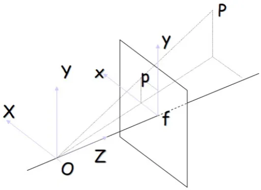
2.1.1 Camera Model

We use the pinhole model to describe the projection of a point into the camera. In the pinhole camera model, the camera is described as a box with a small hole in the front side. Each point in the object is projected into the image based on the principle of collinearity, where the points are projected by a straight line through the camera center (the hole in the front side). This model can be described with a coordinate of (O, x, y, z) where O

represents the camera center. Parameterx andy form a plane that is parallel to with the image plane while the z-axis is perpendicular to the image plane.

(18)

[image:18.595.134.391.129.316.2]

6 Background & Motivation

Figure 2.1: Example of a pinhole model

Intrinsic parameters are used to describe the perspective projection inside the camera. In order to get the relationship between a point in camera coordinatePc(x, y, z)T and the corresponding point on camera retina p(x, y,1)T, an intermediate plane is introduced. It is parallel to the camera´s retina with a unit distance. The points on the normalized plane are described in homogeneous coordinate as ˆp(u, v)T _{and the corresponding homogenous}

projection is described as

ˆ

p= 1

zPc (2.1)

and the point on the image plane is describe as :

p=Kˆp (2.2)

Where the matrixK is described as the camera matrix:

K=



fx0 alphafycfx cxcy

0 0 1



 (2.3)

The vectorfcis the focal length in pixel unit while the vectorccrepresent the principal point coordinates in pixel unit. alphac is the skew coeﬃcient deﬁning the angle between

the x and y pixel axes stored in the scalar.

2.1.2 Camera tracking and Mapping

The orientation and position of the camera is represented as a 3×3 rotation matrixRand a 3×1 translation matrixt while [R|t] describes the extrinsic camera parameter matrix. The transformation of a pointP from Camera 1 to Camera 2 can be deﬁned as:

P′ =R2₁P+t2₁→Pˆ′ =

[

R2₁ t2₁ 0 1

]

ˆ

(19)

§2.1 Structure From Motion 7

wherePˆ is the point in homogeneous coordinate andP′,Pˆ′ are the projected position respectively.

In order to derive the transformation matrix, the ﬁrst step is to match correspon-dences between images. As previously described, traditional methods extract sparse fea-tures as key-points and do feature matching between key-points sets to obtain correspon-dences. There are many types of features can be used here like ORB[12], SURF[13], BRISK[14]...Each type of feature will derive a description of the feature and the matching can be done by comparing the similarity between the descriptors. To obtain the geometric relation between two images directly without the need for retrieving the depth of points, the fundamental matrix is introduced. The fundamental is a 3×3 matrix where

0=x′Fx (2.5)

xis a point in one image while x′ is the correspondence point in another image. We further introduce the essential matrix where:

E=K−1FK (2.6)

And the essential matrixEcan be decomposed intoR,tas described in [15]. However, for monocular cameras, the translation only determines the direction of the real translation and the scale is not observable.

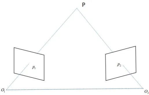
For a sparse feature based algorithm, the mapping is usually done by generating a point cloud of the feature points. In order to obtain the 3D position from a 2D observation, another observation is required and we do triangulation to estimate the depth of the point. Assume the position of a point P in the coordinate in the ﬁrst camera, and the transformation from the ﬁrst camera to the second camera is [R|t].The observation ofPin both camera is p1 and p2. The position of the pointPcan be easily obtained by solving the equation:

Λ2K−1p2 = Λ1 [

R2₁ t2₁ 0 1

]

K−1p1 (2.7)

where Λ1 and Λ2 are the scaling factor of the point observationp1 and p2. The equation

can be reorganized in to the format of Ax=0 and solved using SVD decomposition as shown in [15]. After triangulation, the 3D position of the points and the camera position is usually further optimized using bundle adjustment. Bundle adjustment is a non-linear reﬁnement algorithm which minimizes the overall cost of the errors. For most sparse feature based method the cost function is derived as the re-projection error of the 3D points into the images. The re-projection of a 3D point iinto a camera j can be derived as:

p(i,j)′ =K

[

Rj tj 0 1

]

Pi (2.8)

As the observation of point i in camera j is mij and the image is on the retina plane wherep0[3] = 1 the ﬁnal reprojection error can be written as

Ei,j =||

p(i,j)′

(20)

[image:20.595.133.391.109.274.2]

Figure 2.2: Ideal relationship of the triangulation with two camera

Pi observed in qi views where the relative transformation from the world coordinate to the observing camera coordinatej isTj. The ﬁnal equation of the bundle adjustment can be written as

argc_min{P1...Pn,T1...Tn}= i<n

∑

i=0

j<q∑i

j=0

Ei,j (2.10)

2.2 State-of-Art

Sparse feature based structure from motion is a very popular direction in research and there are many successful systems in the literature. This section gives some brief introduction of some start-of art structure from motion pipelines.

(21)

§2.3 Motivation 9

Bundler [17][18] is another open source library for Structure from motion. Diﬀerent from ORB-SLAM, bundler doesn’t require continuity of the input which means the input does not necessarily capture by the same camera in a sequence. This gives the advantage that bundler can use any image found online for the reconstruction. For each image, it computes the 3D camera position and registers it to the map. With the given transforma-tion between cameras, the 3D positransforma-tion of the image point can be recovered. In bundler, the scene is reconstructed with points and lines in the image. Bundler uses SIFT features which means it can’t run in real-time and it can take a lot of time depending on the size of the dataset.

2.3 Motivation

Curve-based geometric incidence relations have since ever intrigued the structure-from-motion community. For example, rather than solving the relative pose problem from points correspondences [10, 11], early works such as [19] and Lateron [20] and [21] looked into the possibility of using curves and surface tangents to solve the stereo calibration problem. However, the presented constraints for solving geometric computer vision problems are easily inﬂuenced by noise, and not practically useful. In order to improve the quality of curve-based structure from motion, further works, therefore, looked at special types of curves such as straight lines and cones, respectively [22, 23].

Our primary interest is the solution of structure-from-motion over many frames and observations. Point-based solutions are very mature from both theoretical [15] and prac-tical perspectives [24]. However, point-based representations are somewhat unsatisfying as they simply do not present a complete, visually appealing result. It is therefore natural that the structure-from-motion community has been striving for higher-level formulations that are able to return fully dense surface estimates [8]. Fully dense estimation is however very computationally demanding, which is why a compromise in the form of line based rep-resentations has also received signiﬁcant attention from the community [2, 25]. Lines are however not a general model for representing the environment, they fail in environments where the majority of edges are bent. [26, 27, 28, 29] provide a solution to this problem by introducing curve-based representations of the environment, such as sub-division curves, non-rational B-splines, and implicit representations via 3D probability distributions. How-ever, they do not exploit the edge measurements to improve on the quality of the pose estimations as well, as they do not optimize the curves and poses in a joint optimization process.

Full bundle adjustment over general curve models and camera poses has first been shown in [30]. The approach, however, suffers from a bias that occurs when the model is only partially observed. [31] discusses this problem in detail, and presents a lifting approach that transparently handles missing data. [32] solves the problem by modeling curves as a set of shorter line segments, and [33] models the occlusions explicitly. While [31] is the most related to our approach, the lifted formulation is computationally demanding, the work does not discuss the fully automatic establishment of a correspondence graph that would enable fully automatic incremental structure-from-motion. Our main contribution is an efficient, fully automatic solution to this problem, thus enabling automatic curve-based structure from motion in larger scale environments.

(22)

(23)

Chapter 3

Line based Structure from Motion

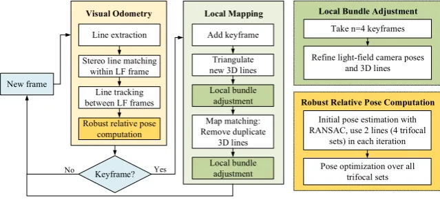
While most monocular visual SLAM frameworks rely on sparse key-points, it has long been acknowledged that lines also represent a higher-order feature with high accuracy and has been proven that they have good repeatability and abundant availability in man-made environments. However, the back-projection of a 2D line measurement is a plane that intersects with the camera center. For any 2D-2D line correspondence between two views, these planes will generally intersect in a 3D line, independently of the relative camera pose. That means a correspondence between two points of view will have no constraint to the camera poses which means at least three views are required to recover the geometric relationship between cameras and this can then be recovered using trifocal tensor geometry [41]. The present chapter also introduces line-based bundle adjustment, the next logical extension to the point-based case.As indicated in [42], using a single camera is most likely insufficient for doing purely line based motion estimation which ,in the end, make us to build a light-field camera for experiment. The goal here essentially consists of real-time visual simultaneous localization and mapping (VSLAM) using line based features and only a system overview is shown in figure 3.1. Instead of using a monocular camera, we use a light-field camera with nine cameras where each of the cameras is calibrated and the relative poses between the cameras is fixed. This chapter is organized as follow: section 3.1 gives a brief introduction of the trifocal tensor geometry which can be used to bootstrap structure-from-motion problems based on lines. Then, in section 3.2, we will demonstrate our back-end line-based bundle adjustment.

New frame

Keyframe?

Visual Odometry

Line extraction

Stereo line matching within LF frame

Line tracking between LF frames

Robust relative pose computation

Local Mapping

Triangulate new 3D lines Add keyframe Local bundle adjustment Map matching: Remove duplicate 3D lines Local bundle adjustment

Robust Relative Pose Computation

Initial pose estimation with RANSAC, use 2 lines (4 trifocal

sets) in each iteration

Pose optimization over all trifocal sets

Local Bundle Adjustment

Refine light-field camera poses and 3D lines Take n=4 keyframes

[image:23.595.171.491.580.725.2]

No Yes

Figure 3.1: The system is originally designed for light-ﬁeld cameras. Here only provide a brief overview of tri-focal tensor based bootstrapping in the front-end and the representation of lines and line-based bundle adjustment in the back-end

(24)

12 Line based Structure from Motion

3.1 Short review of trifocal tensor geometry

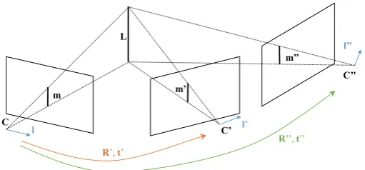
A trifocal tensor describe the geometry relationship of a straight line observed in three views[15]. Suppose a lineLin 3D space is imaged as the corresponding tripletm↔m′ ↔ m′′ across three perspective views, which are indicated in Figure 3.1 by their centers C, C′, and C′′. Trifocal tensor geometry describes the existence of three 3×3 matrices Si (or alternatively a cubic tensor of size 3) that permit the reconstruction of the three coordinates of the line measurement in the ﬁrst view, respectively. Calling the result q, this line transfer is given by

qT =m′T[S1,S2,S3]m ′′

(3.1)

Sinceqideally has to be proportional to the measured line in the ﬁrst view mwe can easily derive the trifocal tensor incidence relation

m′T[S1,S2,S3]m′′[m]_× =0T (3.2)

The trifocal tensor can be described as a function of the three camera matricesP,P′, andP′′. Before proceeding, we ﬁrst move to normalised coordinates given that we assume to be in the calibrated case.We start with normalising the line measurements m that satisfy the equationxT_m_{= 0 for any image point} _x _{along the line. Deﬁning}_K_{to be the}

matrix of intrinsic camera parameters, the equation can be easily rewritten as

xTm= 0⇒xTK−TKTm= 0→(K−1x)T(KTm) = 0 (3.3)

The normalised line coordinates are therefore given by l = KTm, and it is easily recognised that they also correspond to the normal vector of the 3D plane spanned by the 3D line L and the camera center C. Choosing the ﬁrst view to be the reference, the camera matrices in the calibrated case are given by

P= [I|0], P′ = [R′|t′], P′′ = [R′′|t′′] (3.4)

wheret′,R′ = [r′₁ r′₂r′₃] andt′′,R′′= [r′′₁ r′′₂ r′′₃] are the euclidean parameters that per-mit the transformation of points from the ﬁrst to the second and the ﬁrst to the third camera frame. Given its general form taken from [15], the trifocal tensor [T1T2 T3] that

satisﬁes the incidence relation in the calibrated case

(l′T[T1, T2, T3]l

′′

)[l]_×=0T (3.5)

is ﬁnally given by

Ti =r

′

it

′′_T

−t′r′′_iT (3.6)

Let us assume a lineLhas been observed inncameras where the extrinsic calibration parameters are given byciwhile the relative pose between any two camera is described as

{

tj_i,Rj_i

}

, which transform points from theithview tojthview. The geometry is illustrated in Figure 3.1. Any three distinct views, say c1,c2 and c3, selected from the observations

(25)

§3.2 Parameterization and back-end optimization 13

L

m m’

m’’

C

C’

C’’

l l’

l’’

R’, t’

[image:25.595.202.458.102.221.2]

R’’, t’’

Figure 3.2: Multiple-view geometry of 3D line observations.

relative pose between the third and the ﬁrst view of the trifocal set. It is however clear that a single line correspondence is not enough to fully constrain the relative pose. We use in total four line correspondences, from which we can obtain 4×3 constraints on the motion parameters. With a total of 12 equations that are linear in the parameters t and R, we obtain a ﬁrst solver by a simple linear solution, which can be used for bootstrapping our solution. Note that, in order to ensure that the rotation is a proper rotation matrix, we project the linear solution onto the nearest orthonormal matrix via a simple SVD. The lines can be recovered by extracting the two-dimensional null-space of the normalized line measurements in the image plane.

3.2 Parameterization and back-end optimization

As we already explained the front-end, this section shows how do we parameterize the lines as well as how we optimize them during bundle adjustment. Our local mapping module performs optimization of all variables over a window of n most recent keyframes. This includes the poses of the frames as well as all parameters of 3D lines for which there exist at least two observations inside the window of considered frames. The procedure is commonly known as local or windowed bundle adjustment. After a ﬁrst execution terminates, we run a map matching procedure in which we seek further correspondences between the current frame and the 3D lines, directly. After all correspondences have been added, we conclude with another round of local bundle adjustment.

An important question when applying bundle adjustment is how exactly to parametrize the optimized variables. Taking the camera pose in the calibrated case as an example, the diﬃculty lies in making sure that the orientation variable remains a point on the special-orthogonal groupSO(3), either through a minimal, implicit parametrization or by explicitly adding constraints to the optimization. In order to remain free of side-constraints, we simply choose the minimal Cayley parameters to represent the orientation of each frame. Furthermore, in order to ensure that we remain far away from 180 rotations for which|| [x y z]T||→ ∞, we optimize pose changes from the initial absolute pose of each frame rather than the absolute pose directly.

(26)

the two planes without being contained in it. With strong ties to [2], we propose a less restrictive minimal parametrization of the 3D lines for back-end optimization. Sincedand mare orthogonal, they can notably be parametrized as the ﬁrst two columns of a rotation matrix that again is represented as a function of Cayley parameters [43]. The fact that the moment vectormdoes not have unit norm is furthermore reﬂected by multiplying the second column of this matrix by a scale parameter s. We obtain

[

d, m]= 1

1 +x2₊_y2₊_z2    1 +x

2₋_y2₋_z2

2xy+ 2z

2xz−2y



, s



1−2xxy2+−y22z−z2

2yz+ 2x

  

. (3.7)

We furthermore switch to local optimization by adding a starting orientation R0 = [d0 m0

||m0||

(

d0× m0

||m0||

)

]and a starting line moments0to the parametrization, thus resulting in

[d,m] =R0

1

1 +x2₊_y2₊_z2    1 +x

2₋_y2₋_z2

2xy+ 2z

2xz−2y



, (s0+s)



1−2xxy2+−y22z−z2

2yz+ 2x

    (3.8)

As required, this parametrization has only 4 degrees of freedom, and implicitly enforces all side-constraints on the Pl¨ucker line coordinates.

We conclude the exposition of our line-based bundle adjustment back-end by explaining the reprojection error of every 3D line into every frame where a measurement is available. Measurements are notably given by two endpoints p1 and p2 while our 3D lines are

parametrized as inﬁnitely long. The reprojection error is simply given by the sum of the two squared orthogonal distances between the endpoints and the reprojected line. For simplicity, we sample two points from the lines asP1 =d×mandP2=d×m+dwhere

d and m derived from equation 3.8. For a lineLi observed in the jth camera where the

projection from the world coordinate to the camera coordinate derived asπj, the direction

of the projected line can be derived as

n′_ij= [nx, ny]T =µ(πj(p2)−πj(p1)) (3.9)

whereµ(x) return the normalized vector x

µ(x) = x

||x|| (3.10)

The normal direction of the projected line can be derived as

nij= [−ny, nx]T (3.11)

With a reference point of the projected line can be founded as C = π(p2)−π(p1)

2 the

cost of the reprojected line becomes

eij = [nijT(p1−C)]2+ [nijT(p2−C)]2 (3.12)

And the ﬁnal cost becomes

E=∑

ij

(27)

§3.3 Result 15

Note that, in contrast to [3, 44], we employ a genuine, virtually infinite line representa-tion in 3D rather than two end-points. In turn, we utilize end-points where they naturally occur, namely for our measurements extracted in the image plane. This appears to be a more logical definition, as end-points defined in 3D could easily collapse and produce a zero residual.

3.3 Result

As illustrated in [45], even a stereo camera has difficulties in solving the line-based structure from motion problem (depending on the orientation of the base-line). Therefore, we used a light-field camera with a 3x3 matrix arrangement of cameras. Comparing our complete light-field SLAM pipeline on common benchmark datasets is difficult since none of them provides images captured by a plenoptic cam-era. Fortunately, the realistic synthetic benchmark given by the ICL-NUIM datasets [1] enables us to render novel views as captured by a light-field camera matrix. We define a virtual 3×3 camera matrix with 0.1m baselines while keeping the standard intrinsic parameters unchanged and render new views for two living room sequences for which suf-ficient lines can be observed. We compare our framework against multiple state-of-the-art solutions from the literature [16, 46, 47, 48, 49, 50]. We evaluate the absolute trajectory error using the tools provided by the TUM RGBD-SLAM benchmark [51] (see reference for detailed definition), and summarize the median values over 50 runs in Table 3.1. Example views of the environment with overlaid line reconstructions as well as the final trajectory are illustrated in Figure 3.4(b). Note that the sequences have no obvious loop, hence the question of whether or not loop closure is performed in the pipeline is irrelevant.

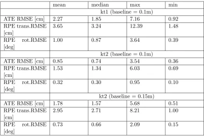
[image:27.595.225.438.595.757.2]

Drift is hardly observable, and the high accuracy is underlined by numbers. We rival even state-of-the-art RGBD-SLAM solutions, and outperform all comparison algorithms on sequence kt2 by returning a sub-centimeter median absolute trajectory error. Further details about the results obtained by our method including the mean, median, maximum, and minimum errors of both the absolute trajectory error and the relative pose error can be found in Table 3.2. Even if changing the intra-light-field baselines to a different value, sub-centimeter accuracy remains achievable (though we confirm that there is of course only one optimal baseline for a given average scene depth).

(28)

Sequence Ours(0.1m base-line) ORB-SLAM2 (stereo)[16] ORB-SLAM2(RGBD)[16] Elastic Fu-sion [46]

kt1 1.9 8.6 17.1 0.9

kt2 0.7 6.8 1.9 1.4

Sequence DVO-SLAM [47] Endres et al. [48] MRSMap [49] Kintinuous [50]

kt1 2.9 0.8 22.8 0.5

[image:28.595.52.476.99.215.2]

kt2 19.1 1.8 18.9 1.0

Table 3.1: Median absolute trajectory errors averaged over 50 runs on ICL-NUIM sequenceskt1

andkt2.

-0.5 0 0.5 1 1.5 2

[image:28.595.87.443.257.409.2]

x [m] -1.5 -1 -0.5 0 0.5 1 z [m] ground truth light field case stereo case (part1) stereo case (part2)

Figure 3.4: Example 3D lines reconstructed by our light-field SLAM pipeline on the synthetic ICL-NUIM living room dataset kt2. The right figure shows a ground-floor projection of the estimated trajectory overlaid on groundtruth. The figure furthermore includes results obtained by using only two sub-views of the light-field camera with diagonal baseline. The trajectory splits into two parts because of tracking loss.

mean median max min

kt1 (baseline = 0.1m)

ATE RMSE [cm] 2.27 1.85 7.16 0.92

RPE trans.RMSE [cm]

3.65 3.24 12.39 1.48

RPE rot.RMSE [deg]

1.00 0.87 3.64 0.39

ATE RMSE [cm] 0.85 0.74 3.54 0.36

RPE trans.RMSE [cm]

1.53 1.34 6.03 0.69

RPE rot.RMSE [deg]

0.32 0.30 0.95 0.10

ATE RMSE [cm] 1.78 1.57 5.68 0.51

RPE trans.RMSE [cm]

2.95 2.71 8.21 1.00

RPE rot.RMSE [deg]

0.73 0.66 2.09 0.15

[image:28.595.63.466.496.765.2]

(29)

Chapter 4

Bezier spline based

parameterization and bundle

adjustment

As already demonstrated the method of using straight lines as a higher order param-eterization of the environment in the previous chapter, there are obvious limitation of straight lines: it is impossible to represent curves which are commonly distributed in nature environments. In this chapter, we explore the possibility of using a even higher order representation of the environment where we use Bezier splines to achieve free form curve parameterization. As a combination of the two paper mentioned in Section 1, this chapter is divided into two self-contain sub-chapter where the first one works on a simpler scenario which assumes that contours are placed on a planar scene and the second one focuses on a fully free form contour representation. This chapter is organized as follow: We first give a general background information of Bezier in Section 4.1, Section 4.2 then presents the contribution of using Bézier spline with a planar scene. In the end, Section 4.3.2 demonstrate how our main contribution of the Bézier spline based structure from motion pipeline.

4.1 B´

ezier splines as a higher-order curve model

Different from the traditional map representation which uses points for map representation, we aim at using Bézier splines and thus reach a more complete, higher order representation of the environment. A Bézier-spline is a continuous curve expression parametrized as a function of control points and a continuous curve parameter t. Every point on the curve can be obtained by referring to a unique value of t. The general definition of a Bézier spline is:

B(t) =

k

∑

i=0

bi,kPi, (4.1)

wherebi,k =

(

k i

)

ti(1−t)k−i and

(

k i

)

= _i_!(_kk₋!_i_)!. Pi is the ith control point of the B´ezier

curve, andk is the order of the curve.

Besides compactness, the choice of Bézier splines is motivated by their simple geometric meaning: the first and last control points are simply the beginning and ending point of the curve while the directions from the first control point to the second and the fourth control point to the third are equal to the local gradient at the beginning and the end

(30)

18 Bezier spline based parameterization and bundle adjustment

of the curve. As we will see, this clear geometric meaning facilitates initialization and regularization of parameters. Furthermore, Bézier curves parameters are invariant with respect to affine transformations, which means that the transformation of a Bézier curve between different coordinate frames is done by simply applying the same transformation to its control points. Furthermore, Bézier splines provide implicit smoothness and a scale invariant density of points along the curve by simply adjusting the step-size of t.

4.1.1 Smooth polyb´eziers

In our work, we use cubic B´ezier splines for representing curves as they are a powerful representation allowing for independent spatial gradients at the beginning and the end of the curve. Cubic splines employ four control pointsPi, hence k= 3, and

B(t) = (1−t)3P0+ 3(1−t)2tP1+ 3(1−t)t2P2+t3P3. (4.2)

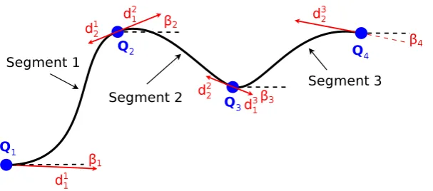
A single cubic Bézier spline is unable to fit arbitrarily complex contours. We overcome this problem by borrowing a simple idea from computer graphics: composite, piece-wise Bézier curves (i.e. so-called polybéziers). As indicated in Figure 4.1, polybéziers separate a contour into multiple segments where every segment is represented by a single Bézier spline of limited order. Composite splines stay continuous by simply sharing the ending point of a segment with the starting point of the subsequent segment. Moreover, in order to maintain smoothness, we furthermore make sure that the gradient at the end of one segment coincides with the spatial gradient at the beginning of the next.

Imposing these constraints is simply done by making the control points a function of other latent variables that are shared among neighbouring segments. On one hand, the continuity simply requires the ﬁrst control point of one segment to be equal to the last control point of the previous segment. Let Pi₀. . .Pi₃ be the control points of segment i. Furthermore, let the ﬁrst control point of a segment also be denoted by Qi. We obtain

Pi₀ = Qi and Pi3 =Qi+1. On the other hand, sharing the gradient is made possible by

explicitly introducing the local direction at the beginning of each segment, denoted vi.

vi is a 3-vector constrained to unit-norm, which means it is a spatial direction with two

degrees of freedom only. Since the second control point by deﬁnition lies in the direction of the local gradient at the ﬁrst control point, it may be parametrised asPi₁=Qi+di1vi.

In order to guarantee smoothness, the third control point of segmentiin turn becomes a function of the gradient at the beginning of the next segment, i.e. Pi

2 =Qi+1−di2vi+1.

In summary, an arbitrary curve is given by a sequence of parameters Qi, vi, and

{di₁, di₂}. By sharing parameters between neighboring segments, a 3D composite B´ezier curve is represented as a sequence of cubic B´ezier segments where

Pi₀=Qi,Pi1=Qi+di1vi,P2i =Qi+1−di2vi+1,Pi3 =Qi+1. (4.3)

We parametrize the normal vectorsviminimally by making them a function of two rotation

angles θi, which avoids the addition of side-constraints during optimization. However, in

(31)

[image:31.595.183.487.122.256.2]

§4.2 Planar B´ezier Spline 19

Figure 4.1: Planar example of a smooth curve parametrization with 3 B´ezier spline segments.

4.2 Planar B´

ezier Spline

We start with a simple scenario where all contours are placed on a planar scene. We use a sparse point-based method to bootstrap the problem and giving an initial guess of the camera poses. Then we use a Bézier spline based method to further refine the accuracy of the pose estimation. As previously described, we represent each curve with a sequence of Bézier segments rather than one long segment with many control points. We extract the edges in the images using canny edges detection [40] and split them into segments of the same length of pixels. For planar scenario, there is no need to represent the curves in full 3D space so we replace thevi and vi+1 in equation 4.3 with only one gradient ϕi and

ϕi+1. Therefore, an example of a curve with 3 B´ezier spline segments on a planar case can

be indicated in Figure 4.1. Let us denote the sequence of starting and ending points of the curve segments with {Q1,· · ·,Qn}. Let segmentisimply be the segment between Qi

and Qi+1. The control points {

Pi₁,· · ·,Pi₄}of segment iare then given by:

Pi₀ =Qi,Pi1 =Qi+di1 [

cosϕi

sinϕi

]

,Pi₂=Qi+1−di2 [

cosϕi+1

sinϕi+1 ]

,Pi₃=Qi+1 (4.4)

4.2.1 Incremental sparse initialization

The entire sparse initialization part relies on local invariant keypoint extraction and match-ing in order to compute an initial guess of camera poses as well as the relative positionmatch-ing of the ground plane. In case of a planar scene, the mapping of points from one image to another can be easily expressed by a homography transformation [15]. We, therefore, boot-strap the sparse computation by first collecting three frames with sufficient frame-to-frame disparity (called keyframe), and then find their relative pose by a robust computation of theplanar homography between these frames. We use three frames because the subsequen-t decomposisubsequen-tion of subsequen-the homography insubsequen-to relasubsequen-tive rosubsequen-tasubsequen-tion, subsequen-translasubsequen-tion, and plane normal leads to two possible solutions [52]. In order to resolve the ambiguity, we simply compute two planar homographies for distinct pairs of frames of the first three keyframes and then compare the similarity of the plane normal vectors after rotating them into one common frame.

(32)

[image:32.595.158.370.121.281.2]

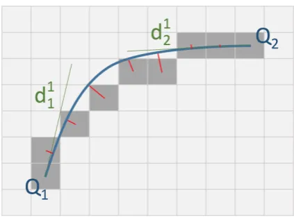
Figure 4.2: Example of a spline segment. The spline initialization consists of minimizing the sum of orthogonal distances from each point on the edge to the spline (in red) overd1

1andd12.

of the ground plane is aligned with the vertical axis ez, and the height of the plane is

z= 0. All points that have been identified as inliers during the robust planar homography computation can furthermore—since effectively lying on the ground plane—be initialized by simply intersecting the spatial measurement ray from any of the first three keyframes with the ground plane. Subsequent frames can now be aligned to the existing sparse background model by simple robust camera resectioning. In our work, we use P3P [53] embedded into Ransac [54] followed by nonlinear optimization to align subsequent frames with the existing model.

We keep deﬁning and storing keyframes during tracking whenever the frame-to-frame disparity exceeds a given threshold. We furthermore keep adding new 3D points to the background model as parts of the background may have been occluded in earlier frames. We notably use the result from the silhouette extraction to deﬁne whether or not a point belongs to the background. Points keep being added to the background by simply inter-secting spatial rays with the background plane. The sparse tracking and mapping part is concluded by a windowed bundle adjustment implementation that optimizes the 6 DoF pose of every keyframe, as well as the 2 DoF position of every point on the background plane.

4.2.2 B´ezier spline parameter initialization

The initialization of a Bézier spline segment turns out to be easy. We first initialize them in the image. An edge is defined as a set of pixels C = {p1,· · ·,pl}. The first and

last control points of each B´ezier spline segment (i.e. the sequence {Q1,· · ·,Qn}) are

simply initialized by subsampling Cwith regularly spaced points. The density of points is deﬁned by considering the local curvature: The higher the curvature, the smaller the distance between Qi and Qi+1. The local gradients {ϕi,· · ·, ϕi+1} can also be estimated

straight from the data. The only parameters that remain to be initialized are di₁ and

di₂. They can be initialized for each segment individually by searching along the gradient directions nearQi and Qi+1.

Substituting (4.4) in (4.2) and considering Qi, Qi+1, ϕi, and ϕi+1 to be ﬁxed, each

B´ezier spline segment Bi can be regarded as a function of the three scalars di1,di2 and t.

(33)

initializing the remaining parameters of each segment can be formulated as

{

ˆ

di₁,dˆi₂

}

=argmin

di

1,di2

p

∑

j=1

min

t ∥Ci[j]−Bi(d

i

1, di2, t)∥2 (4.5)

The energy is also illustrated in Figure 4.2. The minimum location for this energy is simply found by applying Gauss-Newton with numerical Jacobian computation. However, the objective is not entirely trivial to compute, as the derivation depends on an internal minimization over the curve parameter t to find the nearest point on the spline. We re-derive the values fortbefore each Gauss-Newton iteration and notably do so via a simple 1D bisection search. It is intuitively clear that—under the assumption of sufficiently small curvature—finding the optimaltis likely a convex problem, which causes the bi-sectioning search to converge very quickly.

The Bézier spline parameters are first computed in a reference frame and then projected into the ground plane by again intersecting the rays corresponding to the control points in the image with the ground plane itself. As explained above, due to certain transformation invariance properties of Bézier splines, this projection results in sufficiently good initial values for the subsequent global optimization.

(a) (b)

[image:33.595.125.540.438.747.2]

(c) (d)

(34)

4.2.3 Global Optimization

The poses and the background model are finally optimized in a joint curve-based bundle adjustment implementation. Let us assume that there are in totalnBézier spline segments. We define the vector bi =

[

QT_i QT_i₊₁ ϕi ϕi+1 di1 di2 ]T

as the vector of parameters deﬁning the B´ezier spline Bi, which may hence be written as a function B(bi, t). It is

clear that many of the parameters are shared among diﬀerent segments, but we ignore this here for the sake of a simpliﬁed notation. Let us furthermore assume that we have m

camera poses and that the pose of each camera is parametrized by the 6-vector πj. The

objective of our global optimization may then be formulated as minimizing the distance between reprojected samples of each B´ezier spline segment and their closest edge points in each one of the keyframes. If Cj denotes all pixels along an edge in keyframe j, and

η(x,Cj) a function that returns the nearest neighbour ofx within Cj, the optimization objective may be formulated as

{

ˆ

π1,· · ·,πˆm,bˆ1,· · ·,bˆn

}

= (4.6)

argmin

π1,···,πm,b1,···,bn

n ∑ i=1 m ∑ j=1 9 ∑ t=0

∥fπj(B(bi,0.1·t))−η

(

fπj(B(bi,0.1·t)),C

j)_∥2_.

Note that fπj(x) here denotes the transformation from a world frame into the image

plane of a camera with pose parameters πj. Besides the extrinsic pose parameters, this

function also makes use of a suitable camera model with known, pre-calibrated intrinsic parameters (omitted again for the sake of the simplicity of the notation). As can be observed, the internal sum iterates over t and—through the multiplication with 0.1— produces 10 homogeneously distributed samples for reprojection error computation on each B´ezier spline segment. We keep this number ﬁxed, although—in the future—we plan to investigate an adaptive number of sampling points depending on the length of the spline segment. Missing data and occlusions that potentially cause outlier residuals are handled by adding a robust Huber norm to the computation.

In order to compute the nearest neighbour efficiently, we follow [55] and precompute a nearest-neighbour map for the edges of each keyframe. We fix the nearest neighbour point during the numerical Jacobian matrix computation, because a small change in the reprojected location could otherwise lead to very large residual changes due to an unex-pected, significant change of the nearest neighbour if operating at the center between two distinct curves. This furthermore requires a projection of the residual vectors onto the local gradient direction. The interested reader is invited to look at [55] for further details.

4.2.4 Experimental results

We evaluate the planar B´ezier spline based modelling using a self-captured dataset of a planar target with a curve-rich texture. We print out a structured texture—a zebra pattern—for use as a ground. We use a consumer grade, hand-held camera to simply capture a continuous sequence of images while moving around the target. We evaluate our spline-based background model by comparing it against the edges directly extracted from the original image of the background pattern we printed out. We furthermore ana-lyze the residual error and the optimized trajectory before and after spline-based bundle adjustment.

(35)

[image:35.595.165.498.105.277.2]

Figure 4.4: Data Collection for the experiment

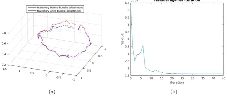
improvement of the camera poses quantitatively. However, as can be observed in Figure 4.5(a), the change in the camera poses is quite substantial. Figure 4.5(b) furthermore shows the overall residual error during each iteration of the non-linear reﬁnement. As can be observed, the residual generally goes down and converges at the end. From this result, we can conclude that the camera poses are optimized as well.

We solve the non-linear least squares problem (4.6) using the Levenberg-Marquardt implementation of the Ceres-Solver library [56]. The latter is an open source C++ library that is able to solve large-scale non-linear optimization problems. The performance of the optimizer is stable as long as the initial guess of the camera poses is not too far oﬀ.

4.2.5 Discussion

The core contribution of our work consists of a successful demonstration of how to use free-form curve models for modeling the environment, and how this can possibly help to increase the accuracy of regular monocular structure from motion. This is demonstrated through the improved dense reconstructions we obtained from our space carving framework. This

(a) (b)

[image:35.595.137.524.581.746.2]

(36)

[image:36.595.68.460.105.244.2]

(a) (b)

Figure 4.6: Left: Two segments of a smooth 3D B´ezier curve. Some of the optimization variables (the control pointsQiand the gradient directionsvi) are shared among adjacent segments. Right:

Epipolar matching with 1D patches. The three best local minima are sub-sequently disambiguated by 2D patch matching. The colors in the right frame indicate the depth of pixels and thus show an example result of semi-dense matching.

work is currently working in a simple senario where most of the background contours are observed in every key-frames and occulision is rarely happens so the following work is obvious: we intend to use the presented B´ezier spline parametrization for reﬁning general non-planar sparse structure-from-motion results and modeling more complex environment.

4.3 3D B´

ezier Spline

As the following work of section 4.2, we are aiming to achieve a fully automatic structure from motion pipeline that using free from Bézier spline for both environment representation and bundle adjustment. In section 4.3.1, we will demonstrate how do we initialize the problem as well as how to we initialize the Bézier spline based mapping. The overall system flow will be shown in subsection 4.3.2 as well as a detailed tracking strategy. The experimental result is shown in section 4.3.3 and a conclusion of this works is given in subsection 4.3.4

4.3.1 Initialization of B´ezier splines

As we will see in Section 4.3.2, our method relies on a sparse technique to ﬁrst initialize the poses of all frames in a video sequence. We proceed by extracting Canny-edges [40] in each image and grouping them into curves based on simple connectivity and thresholding of local curvature. We then initialize the depth of each pixel on an edge by using a variant of the semi-dense epipolar tracking method presented in [36]. For each pixel within each group, we perform the following steps to recover the depth:

• Find a good reference frame for stereo matching by considering the length of the baseline and the parallelism between the epipolar direction and the local image gradient.

• Extract the epipolar line in the reference frame.

(37)

§4.3 3D B´ezier Spline 25

• Short-list the three best local minima.

• For each local minimum, perform a 2D patch comparison to ﬁnd the best.

• Minimise the photometric error via sub-pixel reﬁnement of the disparity along the epipolar line.

• Take a robust average among all the depths recovered within a local window.

The procedure is visualised in Figure 4.6(b). Knowing camera poses as well as semi-dense depth maps in each frame, it now becomes possible to initialize the 3D position of points along the curve expressed in world coordinatespw

pw=Rw(dK−1p) +tw (4.7)

whereRw and tw are the rotation and translation transforming a pointpfrom the camera

to the world coordinate frame,Kis the matrix of intrinsic camera parameters, anddif the depth of the point along the principal axis. We transform all points for which a depth has been recovered into 3D, and furthermore separate the contours into segments such that each segment has roughly the same number of pixels. We furthermore assume that each segment can now be correctly represented by a cubic Bézier spline. We finally estimate the control points of each segment by counting the number of pixels composing the segment, sampling an equal number of values for t distributed homogeneously within the interval (0,1), and assuming that the Bézier spline evaluated at those continuous curve parameter values leads exactly to the hypothesised world point. Let us assume that there are m

world points. Under the above assumption, the curve parameter for each one of the points becomes

tk =

k

m−1, k∈ {0, . . . , m−1} (4.8) Using (4.2), we can then ﬁnd the control points by constructing and solving the linear problem



 (1−t0)

3_I ₃₍₁₋_t

0)2tI 3(1−t0)t2I t30I

. . . . . . . . . . . .

(1−tm−1)3I 3(1−tm−1)2tI 3(1−tm−1)t2I t3m₋1I

      P0 P1 P3 P4    =   p. . .w,0

pw,m−1



 (4.9)

Note that the left-hand matrix only depends on a discrete number of homogeneously sampled values fort, and therefore can be computed upfront. To conclude the initialisation, the B´ezier segments are grouped into curves following the same order of the original segments extracted in the image. To enforce continuity and smoothness in the initialised curve, the ﬁrst control point of each segment is simply replaced by the last control point of the previous segment, and the direction at the link point and the distance from the link point are set to

vi = 0.5∗(P(₄i−1)−P₃(i−1))/∥P₄(i−1)−P(₃i−1)∥