Chapter 4
Apriori
Hiroshi Motoda and Kouzou Ohara
Contents
4.1 Introduction . . . . 62
4.2 Algorithm Description . . . . 62
4.2.1 Mining Frequent Patterns and Association Rules . . . . 62
4.2.1.1 Apriori . . . . 63
4.2.1.2 AprioriTid. . . . 66
4.2.2 Mining Sequential Patterns . . . . 67
4.2.2.1 AprioriAll . . . . 68
4.2.3 Discussion. . . .69
4.3 Discussion on Available Software Implementations . . . . 70
4.4 Two Illustrative Examples . . . . 71
4.4.1 Working Examples . . . . 71
4.4.1.1 Frequent Itemset and Association Rule Mining . . . . 71
4.4.1.2 Sequential Pattern Mining. . . . 75
4.4.2 Performance Evaluation . . . . 76
4.5 Advanced Topics. . . . 80
4.5.1 Improvement in Apriori-Type Frequent Pattern Mining . . . . 80
4.5.2 Frequent Pattern Mining Without Candidate Generation . . . . 81
4.5.3 Incremental Approach . . . . 82
4.5.4 Condensed Representation: Closed Patterns and Maximal Patterns . . . . 82
4.5.5 Quantitative Association Rules . . . .84
4.5.6 Using Other Measure of Importance/Interestingness . . . . 84
4.5.7 Class Association Rules . . . . 85
4.5.8 Using Richer Expression: Sequences, Trees, and Graphs . . . . 86
4.6 Summary . . . . 87
4.7 Exercises . . . . 88
4.1
Introduction
Many of the pattern finding algorithms such as those for decision tree building, clas-sification rule induction, and data clustering that are frequently used in data mining have been developed in the machine learning research community. Frequent pattern and association rule mining is one of the few exceptions to this tradition. Its introduc-tion boosted data mining research and its impact is tremendous. The basic algorithms are simple and easy to implement. In this chapter the most fundamental algorithms of frequent pattern and association rule mining, known as Apriori and AprioriTid [3, 4], and Apriori’s extension to sequential pattern mining, known as AprioriAll [6, 5], are explained based on the original papers with working examples, and performance analysis of Apriori is shown using a freely available implementation [1] for a dataset in UCI repository [8]. Since Apriori is so fundamental and the form of database is limited to market transaction, there have been many works for improving compu-tational efficiency, finding more compact representation, and extending the types of data that can be handled. Some of the important works are also briefly described as advanced topics.
4.2
Algorithm Description
4.2.1
Mining Frequent Patterns and Association Rules
One of the most popular data mining approaches is to find frequent itemsets from a transaction dataset and derive association rules. The problem is formally stated as
follows. LetI = {i1,i2, . . . ,im}be a set of items. LetDbe a set of transactions,
where each transaction t is a set of items such that t ⊆ I. Each transaction has a
unique identifier, called itsTID. A transaction t contains X , a set of some items
inI, if X ⊆ t. An association rule is an implication of the form X ⇒ Y , where X ⊂ I,Y ⊂ I, and X ∩Y = ∅. The rule X ⇒Y holds inDwith confidence c
(0≤c≤1) if the fraction of transactions that also contain Y in those which contain
X inDis c. The rule X ⇒Y (and equivalently X∪Y ) has support1s (0≤s≤1) inD
if the fraction of transactions inDthat contain X∪Y is s. Given a set of transactions
D, the problem of mining association rules is to generate all association rules that have support and confidence no less than the user-specified minimum support (called
minsup) and minimum confidence (called minconf), respectively.
Finding frequent2itemsets (itemsets with support no less than minsup) is not
tri-vial because of the computational complexity due to combinatorial explosion. Once
1An alternative support definition is the absolute count of frequency. In this chapter the latter definition is
also used where appropriate.
2The Apriori paper [3] uses “large” to mean “frequent,” but large is often associated with the number of
4.2 Algorithm Description 63
frequent itemsets are obtained, it is straightforward to generate association rules with confidence no less than minconf. Apriori and AprioriTid, proposed by R. Agrawal and R. Srikant, are seminal algorithms that are designed to work for a large transaction dataset [3].
4.2.1.1 Apriori
Apriori is an algorithm to find all sets of items (itemsets) that have support no less than minsup. The support for an itemset is the ratio of the number of transactions that contain the itemset to the total number of transactions. Itemsets that satisfy minimum support constraint are called frequent itemsets. Apriori is characterized as a level-wise complete search (breadth first search) algorithm using anti-monotonicity property of itemsets: “If an itemset is not frequent, any of its superset is never frequent,” which is also called the downward closure property. The algorithm makes multiple passes over the data. In the first pass, the support of individual items is counted and frequent items are determined. In each subsequent pass, a seed set of itemsets found to be frequent in the previous pass is used for generating new potentially frequent itemsets, called
candidate itemsets, and their actual support is counted during the pass over the data.
At the end of the pass, those satisfying minimum support constraint are collected, that is, frequent itemsets are determined, and they become the seed for the next pass. This process is repeated until no new frequent itemsets are found.
By convention, Apriori assumes that items within a transaction or itemset are sorted in lexicographic order. The number of items in an itemset is called its size and an
itemset of size k is called a k-itemset. Let the set of frequent itemsets of size k be Fk
and their candidates be Ck. Both Fkand Ckmaintain a field, support count.
Apriori algorithm is given in Algorithm 4.1. The first pass simply counts item occurrences to determine the frequent 1-itemsets. A subsequent pass consists of two
phases. First, the frequent itemsets Fk−1 found in the (k−1)-th pass are used to
generate the candidate itemsets Ckusing the apriori-gen function. Next, the database
is scanned and the support of candidates in Ckis counted. The subset function is used
for this counting.
The apriori-gen function takes as argument Fk−1, the set of all frequent (k−
1)-itemsets, and returns a superset of the set of all frequent k-itemsets. First, in the join steps, Fk−1is joined with Fk−1.
insert into Ck
select p.fitemset1, p.fitemset2,. . ., p.fitemsetk−1, q.fitemsetk−1 from Fk−1p,Fk−1q
where p.fitemset1 = q.fitemset1, . . . ,p.fitemsetk−2 = q.fitemsetk−2, p.fitemsetk−1<q.fitemsetk−1
Here, Fkp means that the itemset p is a frequent k-itemset, and p.fitemsetkis the
k-th item of the frequent itemset p.
Then, in the prune step, all the itemsets c∈Ckfor which some (k−1)-subset is
Algorithm 4.1 Apriori Algorithm
F1={frequent 1-itemsets};
for (k=2; Fk−1= ∅; k+ +) do begin
Ck =apriori-gen(Fk−1); //New candidates
foreach transaction t∈Ddo begin
Ct =subset(Ck,t); //Candidates contained in t
foreach candidate c∈Ctdo c.count+ +;
end
Fk= {c∈Ck |c.count ≥mi nsup};
end
Answer= ∪kFk;
The subset function takes as arguments Ckand a transaction t, and returns all the
candidate itemsets contained in the transaction t. For fast counting, Apriori adopts
a hash-tree to store the candidate itemsets Ck. Itemsets are stored in leaves. Every
node is initially a leaf node, and the depth of the root node is defined to be 1. When the number of itemsets in a leaf node exceeds a specified threshold, the leaf node is converted to an interior node. An interior node at depth d points to nodes at depth
d +1. Which branch to follow is decided by applying a hash function to the d-th
item of the itemset. Thus, each leaf node is ensured to contain at most a certain number of itemsets (to be precise, this is true only when creating an interior node takes place at depth d smaller than k), and an itemset in the leaf node can be reached by successively hashing each item in the itemset in sequence from the root. Once the hash-tree is constructed, the subset function finds all the candidates contained in a transaction t, starting from the root node. At the root node, every item in t is hashed, and each branch determined is followed one depth down. If a leaf node is reached, itemsets in the leaf that are in the transaction t are searched and those found are made reference to the answer set. If an interior node is reached by hashing the item i , items that come after i in t are hashed recursively until a leaf node is reached. It is evident that itemsets in the leaves that are never reached are not contained in t.
Clearly, any subset of a frequent itemset satisfies the minimum support constraint.
The join operation is equivalent to extending Fk−1with each item in the database and
then deleting those itemsets for which the (k−1)-itemset obtained by deleting the
(k−1)-th item is not in Fk−1. The condition p.fitemsetk−1<q.fitemsetk−1ensures that
no duplication is made. The prune step where all the itemsets whose (k−1)-subsets
are not in Fk−1are deleted from Ckdoes not delete any itemset that could be in Fk.
Thus, Ck⊇Fk, and Apriori algorithm is correct.
4.2 Algorithm Description 65
all nonempty subsets of every frequent itemset f are enumerated and for every such
subset a, a rule of the form a ⇒ ( f −a) is generated if the ratio of support( f ) to
support(a) is at least minconf. Here, note that the confidence of the rule ˆa⇒( f −ˆa)
cannot be larger than the confidence of a⇒( f−a) for any ˆa⊂a. This in turn means
that for a rule ( f−a)⇒a to hold, all rules of the form ( f−ˆa)⇒ˆa must hold. Using
this property, the algorithm to generate association rules is given in Algorithm 4.2.
Algorithm 4.2 Association Rule Generation Algorithm
H1= ∅//Initialize
foreach; frequent k-itemset fk,k≥2 do begin
A=(k−1)-itemsets ak−1such that ak−1⊂ fk;
foreach ak−1∈ A do begin
con f =support( fk)/support(ak−1); if (con f ≥mi ncon f ) then begin
output the rule ak−1⇒( fk−ak−1)
with confidence=conf and support=support( fk);
add ( fk−ak−1) to H1; end
end
call ap-genrules( fk,H1); end
Procedure ap-genrules( fk: frequent k-itemset, Hm: set of m-item
consequents) if (k >m+1) then begin
Hm+1=apriori-gen(Hm);
foreach hm+1∈ Hm+1do begin
con f =support( fk)/support( fk−hm+1); if (con f ≥mi ncon f ) then
output the rule fk−hm+1⇒hm+1
with confidence=conf and support=support( fk);
else
delete hm+1from Hm+1; end
call ap-genrules( fk,Hm+1); end
4.2.1.2 AprioriTid
AprioriTid is a variation of Apriori. It does not reduce the number of candidates
but it does not use the databaseDfor counting support after the first pass. It uses a
new dataset Ck. Each member of the set Ckis of the form<TID,{I D}>, where
each I D is the identifier of a potentially frequent k-itemset present in the transaction
with identifier TID except k = 1. For k = 1, C1 corresponds to the database D,
although conceptually each item i is replaced by the itemset{i}. The member of Ck
corresponding to a transaction t is<t.TID,{c∈Ck|c contained in t}>.
The intuition for using Ck is that it will be smaller than the databaseDfor large
values of k because some transactions may not contain any candidate k-itemset,
in which case Ck does not have an entry for this transaction, or because very few
candidates may be contained in the transaction and each entry may be smaller than the number of items in the corresponding transaction. AprioriTid algorithm is given in Algorithm 4.3. Here, c[i ] represents the i -th item in k-itemset c.
Algorithm 4.3 AprioriTid Algorithm
F1={frequent 1-itemsets};
C1=databaseD;
for (k=2; Fk−1= ∅; k+ +) do begin
Ck =apriori-gen(Fk−1); //New candidates
Ck = ∅;
foreach entry t∈Ck−1do begin
// determine candidate itemsets in Ckcontained
// in the transaction with identifier t.TID
Ct = {c∈Ck|(c−c[k])∈t.set-of-itemsets∧
(c−c[k−1])∈t.set-of-itemsets}; foreach candidate c∈Ctdo
c.count+ +;
if (Ct = ∅) then Ck+ = t.TID,Ct;
end
Fk= {c∈Ck |c.count ≥mi nsup};
end
Answer= ∪kFk;
Each Ckis stored in a sequential structure. A candidate k-itemset ckin Ckmaintains
two additional fields; generator and extensions, in addition to the field, support count.
The generator field stores the IDs of the two frequent (k−1)-itemsets whose join
generated ck. The extension field stores the IDs of all the (k+1)-candidates that are
extensions of ck. When a candidate ck is generated by joining fk1−1 and fk2−1, their
IDs are saved in the generator field of ckand the ID of ckis added to the extension
field of f1
4.2 Algorithm Description 67
(k−1)-candidates contained in t.TID. For each such candidate ck−1 the extension
field gives Tk, the set of IDs of all the candidate k-itemsets that are extensions of ck−1.
For each ckin Tk, the generator field gives the IDs of the two itemsets that generated ck.
If these itemsets are present in the entry for t.set-of-itemsets, it is concluded that ck
is present in transaction t.TID, and ckis added to Ct.
AprioriTid has an overhead to calculate Ckbut an advantage that Ckcan be stored
in memory when k is large. It is thus expected that Apriori beats AprioriTid in earlier passes (small k) and AprioriTid beats Apriori in later passes (large k). Since both Apriori and AprioriTid use the same candidate generation procedure and therefore count the same itemsets, it is possible to make a combined use of these two algo-rithms in sequence. AprioriHybrid uses Apriori in the initial passes and switches to
AprioriTid when it expects that the set Ckat the end of the pass will fit in memory.
4.2.2
Mining Sequential Patterns
Agrawal and Srikant extended Apriori algorithm to the problem of sequential pattern mining [6]. In Apriori there is no notion of sequence, and thus, the problem of finding which items appear together can be viewed as finding intratransaction patterns. Here, sequence matters and the problem of finding sequential patterns can be viewed as intertransaction patterns.
Each transaction consists of sequence-id, transaction-time, and a set of items. The same sequence-id has no more than one transaction with the same transaction-time. A sequence is an ordered list of itemsets. Thus, a sequence consists of a list of sets of characters (items), rather than being simply a list of characters. The length of a sequence is the number of itemsets in the sequence. A sequence of length k is called a k-sequence. Without loss of generality, the set of items is assumed to be mapped to
a set of contiguous integers, and an itemset i is denoted by (i1i2. . .im) where ijis an
item. A sequence s is denoted bys1s2. . .sn. A sequencea1a2. . .anis contained in
another sequenceb1b2. . .bm(n≤m) if there exist integers i1<i2<· · ·<insuch
that a1⊆bi1,a2 ⊆bi2, . . . ,an ⊆bin. All the transactions with the same sequence-id which are sorted by transaction-time together form a sequence (transaction sequence). A sequence-id supports a sequence s if s is contained in its transaction sequence. The support for a sequence is defined as the fraction of total number of sequence-ids that support this sequence. Likewise, the support for an itemset i is defined as the fraction of sequence-ids that have items in i in any one of their transactions. Note that this definition is different from that used in Apriori. Thus the itemset i and the 1-sequence
ihave the same support.
Given a transaction database D, the problem of mining sequential patterns is to
find the maximal3sequences among all sequences that satisfy a certain user-specified
minimum support constraint. Each such maximal sequence represents a sequential pattern. A sequence satisfying the minimum support constraint is called a frequent
sequence (not necessarily maximal), and an itemset satisfying the minimum support
constraint is called a frequent itemset, or fitemset for short. Any frequent sequence must be a list of fitemsets.
The algorithm consists of five phases: (1) sort phase, (2) fitemset phase, (3) trans-formation phase, (4) sequence phase, and (5) maximal phase. The first three are preprocessing phases and the last one is a postprocessing phase.
In the sort phase, the databaseDis sorted with sequence-id as the major key and
transaction-time as the minor key. In the fitemset phase, the set of all fitemsets is obtained using Apriori algorithm with the corresponding modification of counting a support, and is mapped to a set of contiguous integers. This makes comparing two fitemsets for equality in a constant time. Note that the set of all frequent 1-sequences are simultaneously found in this phase. In the transformation phase, each transaction is replaced by the set of all fitemsets that are in that transaction. If a transaction does not contain any fitemset, it is not retained in the transformed sequence. If a transaction sequence does not contain any fitemset, this sequence is removed from the transformed database, but it is still used in counting the total number of sequence-ids. After the transformation, a transaction sequence is represented by a list of sets of fitemsets.
Each set of fitemsets is represented by{f1, f2, . . . , fn}, where fiis an fitemset. This
transformation is designed for efficiently testing which given frequent sequences are
contained in a transaction sequence. The transformed database is denoted asDT.
The sequence phase is the main part where the frequent sequences are to be enu-merated. Two families of algorithms are proposed: count-all and count-some. They differ in the way the frequent sequences are counted. Count-all algorithm counts all the frequent sequences, including nonmaximal sequences that must be pruned later, whereas count-some algorithm avoids counting sequences which are contained in a longer sequence because the final goal is to obtain only maximal sequences. Agrawal and Srikant developed one count-all algorithm called AprioriAll and two count-some algorithms called AprioriSome and DynamicSome. Here, only AprioriAll is explained due to the space limitation.
In the last maximal phase, maximal sequences are extracted from the set of all frequent sequences. The hash-tree (similar to the one used in the subset function in Apriori) is used to quickly find all subsequences of a given sequence.
4.2.2.1 AprioriAll
The algorithm is given in Algorithm 4.4. In each pass the frequent sequences from the previous pass are used to generate the candidate sequences and then their support is measured by making a pass over the database. At the end of the pass, the support of the candidates is used to determine the frequent sequences.
The apriori-gen-2 function takes as argument Fk−1, the set of all frequent (k−
1)-sequences. First, join operation is performed as
insert into Ck
select p.fitemset1, p.fitemset2,. . . , p.fitemsetk−1, q.fitemsetk−1 from Fk−1p,Fk−1q
4.2 Algorithm Description 69
Algorithm 4.4 AprioriAll Algorithm
F1={frequent 1-sequences}; // Result of fitemset phase for (k=2; Fk−1= ∅; k+ +) do begin
Ck =apriori-gen-2(Fk−1); //New candidate sequences
foreach transaction sequence t ∈DT do begin
Ct =subseq(Ck,t); //Candidate sequences contained in t
foreach candidate c∈Ctdo c.count+ +;
end
Fk= {c∈Ck |c.count ≥mi nsup};
end
Answer=maximal sequences in∪kFk;
then, all the sequences c∈Ckfor which some (k−1)-subsequence is not in Fk−1are
deleted. The subseq function is similar to the subset function in Apriori. As in Apriori,
the candidate sequences Ck are stored in a hash-tree to quickly find all candidates
contained in a transaction sequence. Note that the transformed transaction sequence is a list of sets of fitemsets and all the fitemsets in a set have the same transaction-time, and no more than one transaction with the same transaction-time is allowed for the same sequence-id. This constraint has to be imposed in the subseq function.
4.2.3
Discussion
Both Apriori and AprioriTid need minsup and minconf to be specified in advance. The algorithms have to be rerun each time these values are changed, throwing everything away that was obtained in previous runs. If no appropriate values for these thresholds are known in advance and we want to know how the results change with these values without rerunning the algorithms, the best we can do is to generate and count only those itemsets that appear at least once in the database without duplication and store them all in an efficient way. Note that Apriori generates candidates that do not exist in the database.
Apriori and AprioriTid use a hash-tree to store the candidate itemsets. Another data structure that is often used is a trie-structure [35, 9]. Each node in the depth k of the trie corresponds to a candidate k-itemset and stores the k-th item and the support
of the itemset. As two frequent k-itemsets that share the first (k −1)-itemsets are
siblings below their parent node at the depth k−1 in the trie, the candidate generation
If we go a step further, we can get rid of generating candidate itemsets at all. Further, it is not necessary to enumerate all the frequent itemsets. These topics are discussed in Section 4.5.
Apriori and almost all other association rule minings use two-phase strategy: first mine frequent patterns and then generate association rules. This is not the sole way. Webb’s MagnumOpus uses another strategy that immediately generates a large subset of all association rules [38].
There are direct extensions of the original Apriori family. Use of taxonomy and in-corporating temporal constraint are two examples. Generalized association rules [30] employ a set of user-specified taxonomies, which makes it possible to extract fre-quent itemsets that are expressed by higher concepts even when use of the base level concepts produces only infrequent itemsets. The basic algorithm is to add all ances-tors of each item in a transaction to the transaction and then run Apriori algorithm. Several optimizations can be added to improve efficiency, one example being that the support for an itemset X that contains both an item x and its ancestor ˆx is the
same as the support of the itemset X−ˆx, and thus need not be counted. Generalized
sequential patterns [32] place, in addition to the introduction of taxonomies, time constraints that specify a minimum and/or maximum time period between adjacent elements (itemsets) in a pattern and relax the restrictions that items in an element of a sequential pattern must come from the same transaction by allowing the items to be present in a set of transactions of the same sequence-id whose transaction-times are within a user-specified time window. It also finds all frequent sequential patterns (not limited to maximal sequential patterns). GSP algorithm runs about 20 times faster than AprioriAll, one reason being that GSP counts fewer candidates than AprioriAll.
4.3
Discussion on Available Software Implementations
There are many available implementations of Apriori ranging from free software to commercial products. Here, we will present only three well-known implementations which are freely downloadable via Internet.
The first one is an implementation embedded in the most famous open-source machine learning and data mining toolkit, Weka, provided by the University of Waikato [40]. Apriori in Weka can be used through Weka’s common graphical user interface together with many other algorithms that are available in Weka. The im-plementation includes Weka’s own extensions. For example, minsup is iteratively
decreased from an upper bound Umi nsup to a lower bound Lmi nsup with an interval
δmi nsup. Further, in addition to confidence the metrics lift, leverage, and conviction are
4.4 Two Illustrative Examples 71
The second implementation is the one by Christian Borgelt [1], which is distributed under the terms of the GNU Lesser (Library) General Public License. This imple-mentation is basically a command line application, and some graphical user interfaces are separately available. It essentially follows the flow of the original Apriori, but has its own extensions, too, to make it faster and to reduce its memory use. It employs a trie called the prefix tree to store both transactions and itemsets for efficient support counting [10]. The prefix tree is slightly different from the trie explained in Sub-section 4.2.3. Optionally, the user can choose to use a simple list instead of a prefix tree to store transactions. Furthermore, this implementation can find not only frequent itemsets and association rules, but also closed itemsets, and maximal itemsets. Closed and maximal itemsets are discussed in Section 4.5. In addition, several metrics other than confidence, such as information gain, are also available in this implementation to evaluate and select association rules.
The third implementation is the one by Fence Bodon, which is freely distributed for research purposes [2]. This implementation is also trie-based, similar to Borgelt’s, but adopts a trie with a simpler structure, and computes only frequent itemsets and association rules. It works as a command line application, and accepts four arguments. The first three are mandatory: an input file, including transactions, an output file, and
minsup. The fourth is minconf, which is optional. If minconf is given, association rules
are mined, as well as frequent itemsets; otherwise, it outputs only frequent itemsets. This implementation is written in C++ to provide object-oriented components which can be easily reused to develop other Apriori-based algorithms.
4.4
Two Illustrative Examples
4.4.1
Working Examples
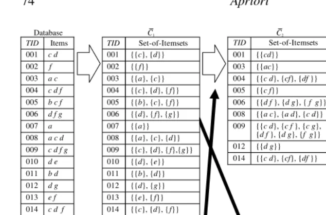
We will illustrate the detailed behavior of the aforementioned algorithms using a small database shown in Table 4.1, where SID and TT mean the sequence-id and transaction-time, respectively. We use this database in both association rule (frequent itemset) mining and maximal sequential pattern mining. In the former case SID and TT are ignored.
4.4.1.1 Frequent Itemset and Association Rule Mining
Suppose that we want to find frequent itemsets under mi nsup=0.2 and association
rules with mi ncon f =0.6.
Apriori (Algorithm 4.1)
Apriori first scans the whole database and derives a set of frequent 1-itemsets
appearing in at least three transactions, F1 = {a,c,d, f,g}. From this F1,
the apriori-gen function derives a set of candidate frequent 2-itemsets C2 =
{ac,ad,a f,ag,cd,c f,cg,d f,dg, f g}. C2consists of all possible pairs of elements
TABLE 4.1
A Transaction Database of the Working ExampleTID SID TT Items
001 1 May 03 c,d
002 1 May 05 f
003 4 May 05 a,c
004 3 May 05 c,d,f
005 2 May 05 b,c, f
006 3 May 06 d, f,g
007 4 May 06 a
008 4 May 07 a,c,d
009 3 May 08 c,d,f,g
010 1 May 08 d,e
011 2 May 08 b,d
012 3 May 09 d,g
013 1 May 09 e,f
014 3 May 10 c,d,f
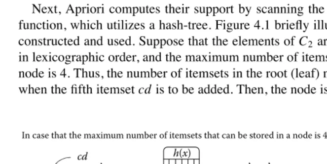
Next, Apriori computes their support by scanning the database using the subset function, which utilizes a hash-tree. Figure 4.1 briefly illustrates how a hash-tree is
constructed and used. Suppose that the elements of C2are added into the hash-tree
in lexicographic order, and the maximum number of itemsets allowed to be in a leaf node is 4. Thus, the number of itemsets in the root (leaf) node exceeds the threshold when the fifth itemset cd is to be added. Then, the node is converted into an interior
In case that the maximum number of itemsets that can be stored in a node is 4.
(b) Check which itemsets are included in a transaction (a) Make a hash-tree
Given Transaction 004 cd
ac ad af ag
df cd cf
cg
h(x) h(x)
c d f c d f c d f
h(x) h(x)
h(x)
h(a) h(c)
cd cd cf df dg fg
cg ac ad
af ag ac adaf ag
dg df fg cd cf
cg ac ad af ag dg fg
cd cf cg ac ad af ag dg
df fg ac ad
af ag
h(c) h(d) h(f) h(a)
h(c) h(d) h(f) h(a)
h(c) h(d) h(f) h(a)
h(a)
h(c) h(d) h(f)
[image:12.612.60.392.399.565.2]4.4 Two Illustrative Examples 73
one, and each itemset branches into the corresponding new leaf node according to the hash value given by the function h(x), where x is an item, the first item in each itemset in this case. We assume that h(x) is given in advance and is common for all nodes. Since the first four itemsets share the same first item a, they fall into the same leaf node, while cd falls into a different one. When checking which of the candidates are included in a transaction, for example, Transaction 004, each item in the transaction is hashed at the root node. For example, by hashing c in cd f , it reaches the second left leaf node, and two itemsets cd and c f are found to be subsets of cd f as shown in the left tree of Figure 4.1(b). Next, by hashing d, d f is found in the third left leaf node (the middle tree), but by hashing f , no subset of cd f is found in the rightmost leaf node (the right tree). As a result, the support counts of these itemsets found, cd, c f , and d f , are increased by 1. Note that, after all the transactions have been processed, the frequencies of the candidates a f and ag are found to be 0. This means that Apriori may generate candidates that do not exist in a given database.
After this support counting, F2 = {cd,c f,d f,dg} is derived. These frequent
2-itemsets in F2are used as the seeds of frequent 3-itemsets. The itemsets cd and c f
in F2sharing the first item c are joined and yield a new candidate cd f by apriori-gen
because d f is also included in F2. The itemsets d f and dg are also joined as well,
but the resulting condidate is pruned because its subset f g is not included in F2.
Consequently, C3, a set of candidate frequent 3-itemsets, consists of cd f only. Then,
Apriori counts its support by scanning the database again, and derives F3 = {cd f}.
No candidate frequent 4-itemsets can be generated from this F3because it contains
only one itemset. Thus, Apriori terminates.
AprioriTid (Algorithm 4.3)
Apriori has to scan the whole database three times to obtain these frequent itemsets, but AprioriTid (Algorithm 4.3) scans it only once for the first pass, and makes and uses
new datasets C1and C2to count the support of candidates in C2and C3, respectively.
Figure 4.2 illustrates how AprioriTid finds frequent itemsets from these datasets. C2
is generated while counting the support of each candidate in C2, whereas C1is
gen-erated directly from the given database. Suppose t = 001,{{c},{d}} ∈C1. Then, a
candidate cd in C2is added to Ctbecause t.set-of-itemsets ({{c},{d}}) contains both
1-itemsets constituting cd. More precisely, cd is added to Ctbecause it is a union of
two 1-itemsets in t, which means Transaction 001 supports cd. No other candidate
is added to Ct as Transaction 001 does not support any other candidate in C2. Then,
the support count of cd is increased by 1, and001,{{cd}}is added to C2. Similarly,
003,{{ac}}is added to C2because Transaction 003 supports ac∈C2, although an
entry corresponding to002,{{f}}of C1 is not because Transaction 002 does not
support any 2-itemsets. Eventually, C2has 9 entries, as shown in Figure 4.2, whose
size is smaller than that of the given database. C3is generated in the same manner
during the support counting of candidates in C3. Since the unique candidate in C3
is cd f , only the three entries of C2, including both cd and c f , whose union is cd f ,
survive in C3. Note that C3is generated, but actually never used because C4becomes
Database C1
F1 C2 F2 C3 F3
C2 C3 Items TID 001 014 013 012 011 010 009 008 007 006 005 004 003 002 c d
c d f e f d g b d d e c d f g a c d a d f g b c f c d f a c f Set-of-Itemsets TID 001 014 013 012 011 010 009 008 007 006 005 004 003 002
{{c}, {d}}
{{c}, {d}, {f}} {{e}, {f}} {{d}, {g}} {{b}, {d}} {{d}, {e}} {{c}, {d}, {f},{g}} {{a}, {c}, {d}} {{a}} {{d}, {f}, {g}} {{b}, {c}, {f}} {{c}, {d}, {f}} {{a}, {c}} {{f}}
{{c d}, {cf}, {df }} 004
{{cd}} 001
{{c d}, {cf}, {df }} 014
{{d g}} 012
{{c d}, {c f }, {c g}, {d f }, {d g}, {f g}} 009
{{a c}, {a d}, {c d}} 008
{{d f }, {d g}, { f g}} 006
{{c f}} 005
{{ac}} 003
Set-of-Itemsets
TID
{{c d f}} 014
{{c d f }} 009
{{c df}} 004
Set-of-Itemsets
TID
3 {c d f }
Support Itemset {c d f }
Itemset 3
{a}
7 {c}
3 {g}
7 {f}
9 {d}
Support Itemset
{c d} {a g} {a f } {a d} {a c}
{ f g} {d g} {c f }
{d f } {c g} Itemset
5 {c d}
3 {d g}
4 {d f }
4 {c f }
[image:14.612.57.392.64.285.2]Support Itemset
Figure 4.2 Example of AprioriTid.
Association rules (Algorithm 4.2)
Next, association rules are generated from the found frequent itemsets according to
Algorithm 4.2 for the given mi ncon f = 0.6. Let us consider frequent 2-itemsets,
cd, c f , d f , and dg, first. It is obvious that only two kinds of rules can be generated
from each itemset. Table 4.2 summarizes the resulting rules and their confidence. The association rules 1 and 8 are the outputs by Algorithm 4.2 because they satisfy the
mi ncon f constraint. The procedure ap-genrules is called for each of these satisfactory
rules, but it outputs nothing because it no longer generates other rules from the 2-itemsets.
Then, Algorithm 4.2 tries to generate association rules from the frequent 3-itemset,
cd f . First, it generates three association rules with 1-item consequent as shown in the
left half of Table 4.3. Algorithm 4.2 returns all of them as they satisfy the mi ncon f
constraint. After that, the procedure ap-genrules is called, taking cd f and{c,d,f}
TABLE 4.2
Association Rules Generated from Frequent2-Itemsets
No. Rule Confidence No. Rule Confidence
1 c⇒d 0.71 5 d ⇒ f 0.44
2 d ⇒c 0.56 6 f ⇒d 0.57
3 c⇒ f 0.57 7 d ⇒g 0.33
[image:14.612.95.354.516.605.2]4.4 Two Illustrative Examples 75
TABLE 4.3
Association Rules Generated from Frequent3-Itemsets
1-Item Consequent 2-Item Consequent
No. Rule Confidence No. Rule Confidence
9 cd ⇒ f 0.60 12 f ⇒cd 0.43
10 c f ⇒d 0.75 13 d⇒c f 0.33
11 d f ⇒c 0.75 14 c⇒d f 0.43
as its arguments. A set of 2-itemsets{cd,c f,d f}is derived by the function
apriori-gen called within ap-apriori-genrules, each of which is used as the consequent of a new association rule. The resulting three rules are shown in the right half of Table 4.3. But, none of them can be the outputs because their confidence is less than the specified
mi ncon f =0.6. Since 3-item consequents cannot be obtained from cd f , ap-genrules
terminates, and Algorithm 4.2 terminates too because F4= ∅.
4.4.1.2 Sequential Pattern Mining
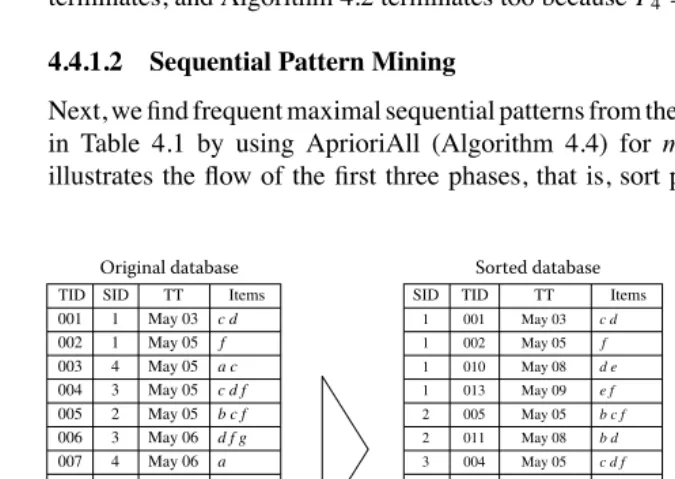
Next, we find frequent maximal sequential patterns from the same transaction database
in Table 4.1 by using AprioriAll (Algorithm 4.4) for minsup = 0.3. Figure 4.3
illustrates the flow of the first three phases, that is, sort phase, fitemset phase, and
Original database Sorted database Frequent itemsets
May 10 May 09 May 09 May 08 May 08 May 08 May 07 May 06 May 06 May 05 May 05 May 05 May 05 May 03 TT 3 1 3 2 1 3 4 4 3 2 3 4 1 1 SID c d 001
c d f
014 e f 013 d g 012 b d 011 d e 010
c d f g
009
a c d
008
a
007
d f g
006
b c f
005
c d f
004 a c 003 f 002 Items TID Transformed database
Fitemset Mapped To (d)
(c f ) (f) (c d )
(c) 2 5 4 1 3
Sequence Transformed sequence
SID After mapping
4 3 2 1
<(a c) (a) (a c d )>
<(c d f) (d f g) (c d f g) (d g) (c d f )> <(b c f ) (b d ) >
<(c d) (f) (d e) (e f )>
<{(c)} {(c), (d) , (cd )}> <{(c), (d), (cd), (f) , (c f)} {(d), (f)} {(c), (d), (cd), (f) , (c f)} {(d)} {(c), (d), (cd), (f) , (c f)}> <{(c), (f), (c f )} {(d)} > <{(c), (d), (c d)} {(f)} {(d)} {(f)}>
<{1} {1, 2 , 3}>
<{1, 2, 3, 4, 5} {2, 4)} {1, 2, 3, 4, 5} {2} {1, 2, 3, 4, 5}> <{1, 2, 3} {4} {2} {4}>
<{1, 4, 5} {2} >
TID TT
SID Items
c d f
May 10 014 3 d g May 09 012 3
c d f g
May 08 009 3
d f g
May 06 006 3
c d f
May 05 004 3 b d May 08 011 2
b c f
May 05 005 2 e f May 09 013 1 d e May 08 010 1 008 007 003 002 001 May 07 May 06 May 05 May 05 May 03 4 4 4 1
1 c d
a c d a a c f
[image:15.612.55.393.346.585.2]TABLE 4.4
Frequent Sequences and Candidate SequencesF1 C2 F2 C3 F3 C4 F4
1 11 12 21 13 31 11 12 111 112 113 114 124 142 1244 1424
2 14 41 15 51 22 13 14 122 132 124 142 144 224 1424 2424
3 23 32 24 42 25 22 32 134 144 222 224 242 324 2244 3424
4 52 33 34 43 35 24 42 242 322 324 342 342 244 2424
5 53 44 45 54 55 52 34 244 422 424 442 424 344 3244
44 522 344 444 3424
transformation phase on this example. In the sort phase, transactions in the database are sorted with sequence-id (SID) as the major key and transaction-time (TT) as the minor key. Then, in the fitemset phase, fitemsets are derived in the similar manner to Apriori. Note that the support of an fitemset is the number of transaction sequences, including the itemset, but not the number of transactions including it. Thus, the
re-sulting set of frequent 1-itemsets in this case is{c,d, f}. In the transformation phase,
each transaction sequence is transformed into a list of sets of fitemsets as shown in the bottom of Figure 4.3 by replacing each transaction in the sequence with a set of fitemsets the transaction contains. Note that the second transaction is dropped in the
transaction sequence 4 because it consists of only one nonfrequent itemset{a}.
AprioriAll generates a set of candidate sequences C2from F1by calling the function
apriori-gen-2. The resulting C2is shown in Table 4.4. The function apriori-gen-2 is
similar to gen, but differs in its join operation: The join operation of
apriori-gen-2 generates two new k-sequences from two (k−1)-sequences whenever they are
joinable, while the join operation of apriori-gen generates only one k-itemset from
two (k−1)-itemsets. For example, when deriving C2, both two sequences12and
21are generated from1and2. In addition,11is also generated by joining the
identical sequence1. This is necessary to generate a sequence in which multiple
occurrences of an fitemset is allowed.
Counting the support of each candidate sequence is done in the similar way as
Apriori using a hash-tree, and F2, a set of frequent 2-sequences, is derived as shown
in Table 4.4. This F2is used to generate a set of candidate sequences C3as well. Note
that from11and12, a 3-sequence112is generated by joining them, but not121
because its subsequence21is not included in F2. This process consisting of the
can-didate generation and support counting is repeated until no more frequent sequences are derived. In this example, since no candidate of 5-sequences can be generated from
F4, F5becomes empty and thus, the iteration terminates. Finally, AprioriAll outputs
1424,2424,3424,11,13, and52as the maximal frequent sequences as
the other frequent sequences are included in one of them.
4.4.2
Performance Evaluation
4.4 Two Illustrative Examples 77
0 5 10 15 20 25 30 35 40 45 50
Runtime (s)
minconf=90% minconf=80% minconf=70% minconf=60% minconf=50%
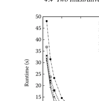
[image:17.612.130.321.66.261.2]0 5 10 15 20 25 30 Minsup (%)
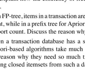
Figure 4.4 Runtime for various minsup and minconf values.
naive implementation closest to the original Apriori. Thus, we disabled its functions of sorting items with respect to their support and of filtering unused items from transactions.
As a benchmark dataset, we used the Mushroom dataset downloadable from UCI Machine Learning Repository [8], which contains 8124 cases with 23 nominal at-tributes including a class attribute. Each case is regarded as a transaction, and each attribute value of each case is converted into an item by joining it with the correspond-ing attribute name, for example, “cap-shape=x,” where cap-shape is an attribute name and x is an attribute value. In 2480 cases, the attribute value of one attribute is miss-ing. Since we ignored missing values, the transactions corresponding to them have 22 items, while the others have 23 items. Some attribute values have different meanings for different attributes. For example, “n” means “none” for the attribute “odor,” while “brown” for “cap-color.” As a result, the number of valid pairs of attribute name and attribute value, that is, number of distinct items, became 118.
Number of association rules (k) 4000
3500
3000
2500
2000
1500
1000
500
0
0 5 10 15 20 25 30 Minsup (%)
[image:18.612.129.322.67.265.2]minconf=90% minconf=80% minconf=70% minconf=60% minconf=50%
Figure 4.5 Number of association rules derived for various minsup and minconf values.
These results show that minsup, or the antimonotonicity property of itemsets, is very effective to prune nonfrequent itemsets.
Next, we show the relation between the runtime and the number of transactions in Figure 4.7. In this evaluation, we copied the original dataset multiple times (up to
Number of frequent itemsets (k)
1000
800
600
400
200
0
0 5 10 15 20 25 30 Support (%)
[image:18.612.131.321.383.579.2]4.4 Two Illustrative Examples 79
minconf=90% minconf=80% minconf=70% minconf=60% minconf=50%
Runtime (s)
45
40
35
30
25
20
15
10
x4 x3
x2 x1
[image:19.612.130.322.65.255.2]Size of the dataset
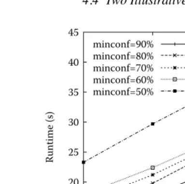
Figure 4.7 Runtime for various sizes of the dataset (minsup=5).
4 times). Note that the fraction of each item remains the same for all datasets, so is the number of resulting association rules (frequent itemsets). Figure 4.7 shows that the runtime linearly increases as the number of transactions becomes larger. Consequently, under a certain distribution of items, minsup is much more influential to the runtime than both minconf and the number of transactions in Apriori.
Finally, we briefly mention association rules mined through the experiments, es-pecially, for convenience, those which have only one item representing the class attribute in the consequent. The class value is either “edible” (e) or “poisonous” (p).
A typical rule found under mi nsup=0.3 and mi ncon f =0.9 is “odor=n gill-size
=b ring-number=o⇒class=e,” which is the simplest one among those whose
consequent is “class=e,” confidence is 1.0, and support is maximum (0.331). This
rule means a mushroom is edible if its order is none, the size of its gill is broad, and the number of its rings is one. The attributes “odor” and “gill-size” appear as the first and the third test nodes, respectively, in the decision tree learned from this dataset by J48, a decision tree learner available in Weka, under its default setting. A similar rule
“odor=n spore-print-color=w gill-size=b⇒class=e” can be derived from the
decision tree and its confidence is 1.0, too, but it is true for only 528 cases, while the association rule is true for 2689 cases. On the other hand, no rule whose confidence
is 1.0 and consequent is “class=p” was found under this setting because mi nsup
was too high. When setting mi nsup=0.2, 470 such rules were found.
rules. More efficient algorithms and better measures are required to find frequent itemsets and interesting association rules, which are the topics of the next section.
4.5
Advanced Topics
Since the first proposal of frequent pattern and association rule mining algorithm by Agrawal and Srikant, there have been many publications on various kinds of im-provements, extensions, and applications, ranging from efficient scalable data mining methodologies, to handling a wide diversity of data types, various extended mining tasks, and a variety of new applications. Some of the important advanced topics are briefly described in this section. There are good tutorials and surveys for frequent pattern mining by Han et al. [16] and Goethals [15] that contain a substantial amount of references.
4.5.1
Improvement in Apriori-Type Frequent Pattern Mining
There have been many attempts to devise more efficient algorithms of frequent itemset mining in the framework of Apriori algorithm in that they generate candidates. These include hash-based technique, partitioning, sampling, and using vertical data format.
Hash-based technique can reduce the size of candidate itemsets. Each itemset is hashed into a corresponding bucket by using an appropriate hash function. Since a bucket can contain different itemsets, if its count is less than a minimum support, these itemsets in the bucket can be removed from the candidate sets. DHP [26] uses this idea.
Partitioning can be used to divide the entire mining problem into n smaller ones [29]. The dataset is divided into n nonoverlapping partitions such that each partition fits into main memory and each partition is mined separately. Since any itemset that is potentially frequent must occur as a frequent itemset in at least one of the partitions, all the frequent itemsets found this way are candidates, which can be checked by accessing the entire dataset only once. Sampling is simply to mine a random sampled small subset of the entire data.
Since there is no guarantee that we can find all the frequent itemsets, normal practice is to use a lower support threshold. Trade-off has to be made between accuracy and efficiency.
4.5 Advanced Topics 81
Algorithm 4.5 FP-Growth Algorithm: F[I ](FP-tree)
F [I ]= ∅;
foreach i ∈Ithat is inDin frequency increasing order do begin
F [I ]=F [I ]∪ {I ∪ {i}}; Di = ∅;
H = ∅;
foreach j ∈IinDsuch that j <i do begin
// ( j is more frequent than i )
Select j for which support (I∪ {i,j})≥mi nsup;
H =H∪ {j}; end
foreach (T i d,X )∈Dwith i ∈ X do
Di =Di∪ {(T i d,{
X\ {i}} ∩H )};
Construct conditional FP-tree fromDi;
Call F [I∪ {i}](conditional FP-tree);
F [I ]=F [I ]∪F [I∪ {i}](conditional FP-tree); end
given a set of candidate itemsets, that their TIDs are available in main memory, which is of course not always the case. However, it is possible to significantly reduce the total size by using a depth-first search. Eclat [43] uses this strategy.
In the depth-first approach, it is necessary to store at most theTIDlist of all
k-itemsets with the same first k−1 items (k−1 prefix) at depth d with k≤d
in the main memory.
4.5.2
Frequent Pattern Mining Without Candidate Generation
by choosing an item in the order of increasing frequency and extracting frequent itemsets that contain the chosen item by recursively calling itself on the conditional FP-tree, that is, FP-tree conditioned to the chosen item. FP-growth is an order of magnitude faster than the original Apriori algorithm. The algorithm of FP-growth
is given in Algorithm 4.5. F[∅](FP-tree) returns all the frequent itemsets. As noted
easily, the divide and conquer strategy mentioned by Han et al. is equivalent to the
depth-first search without candidate generation. TheDiis called i -projected database
and generally much smaller than the FP-tree of the whole database. It is, thus, expected
thatDifits in the main memory even if the latter does not. The idea of pattern growth
can also be applicable to closed itemset mining [27] (see Section 4.5.4) and sequential pattern mining [28] (see Section 4.5.8).
4.5.3
Incremental Approach
When the database is not stationary and a new batch of transactions keeps being added, it happens that some items that were frequent become no more frequent (losers) and some other items that were infrequent become frequent (winners). Rerunning Apriori or any other frequent pattern mining algorithm each time the database is updated is not efficient. The FUP algorithm in [12] provides a way to incrementally update the frequent itemsets using Apriori framework. It works efficiently on the updated
database since the size of the increment databaseDis generally much smaller than
the initial databaseD.
Let Fk, Fk be the frequent k-itemsets inDandD∪D, respectively, and Ckbe
the candidate frequent itemsets inD∪D. At k-th iteration, Ck can be generated
from Fk−1using apriori-gen function. Any itemset in Fkthat contains any one of the
losers of size k−1 (those which are in Fk−1but not in Fk−1) as its subset are filtered
out from Fk without checkingD. Frequency of the remaining itemsets in Fk are
counted overDand those frequent inD∪Dare identified ( A), and excluded from
Ckbecause we know that they are frequent. The remaining itemsets are those not in
Fk. Their frequency is counted overDand those not frequent inDare removed
from Ckbecause we know that they are infrequent inD. Frequency of the remaining
elements in Ckare counted overD∪Dand the frequent ones are retained (B). Fk
is A∪B. As can be seen above, FUP has to scan the updated database for each k, but
the size of the Ckis expected to be very small. The experiment shows that it is only
about 2 to 5% of that of rerunning Apriori for the updated database, and FUP runs 2 to 16 times faster than Apriori.
4.5.4
Condensed Representation: Closed Patterns
and Maximal Patterns
An itemset (pattern) X is a maximal itemset if (1) there exists no itemset Xsuch that
Xis a proper superset of X . An itemset (pattern) X is a closed itemset if (1) there
exists no itemset Xsuch that Xis a proper superset of X and (2) every transaction
containing X also contains X. They are frequent if their support is no less than the
minsup. A closed itemset satisfies I (T(X ))=X , whereT(X )= {t∈D|X ⊆t}and
4.5 Advanced Topics 83
is the same, X is not a closed itemset. A closed itemset is a lossless representation, whereas a maximal itemset is not. Thus, once the closed itemsets are found, all the
frequent itemsets can be derived from them. A rule X ⇒Y is an association rule
on frequent closed itemsets if (1) both X and X ∪Y are frequent closed itemsets,
(2) there does not exist a frequent closed itemset Z such that X ⊂Z ⊂(X∪Y ), and
(3) the confidence of the rule is no less than minconf. The complete set of association rules can be generated once frequent closed itemsets are found.
CLOSET partitions the database and decomposes the problem into a set of subprob-lems, each with the corresponding conditional database, and it is known efficient [27]. First, all the frequent items are derived and sorted in the order of descending support
count as f list= i1,i2, . . . ,in. The j -th subproblem (1≤ j ≤n) is to find the
com-plete set of frequent closed itemsets containing in+1−jbut no ik(for n+1−j<k≤n).
The in+1−jconditional database is the subset of transactions containing in+1−j, where
all the occurrences of infrequent items, item in+1−j, and items following in+1−j in
the f list are omitted. The corresponding FP-tree is generated and used for search. Each subproblem is recursively decomposed if necessary. The frequent closed item-sets are identified from the conditional database using the following properties. If
X is a frequent closed itemset, there is no item appearing in every transaction in
the X -conditional database. If an itemset Y is the maximal set of items appearing in
every transaction in the X -conditional database, and X∪Y is not subsumed by some
already found frequent closed itemset with identical support, X ∪Y is a frequent
closed itemset. As in FP-growth, further optimization is possible.
LCM is another algorithm, known to be the most efficient, to find the closed patterns (itemsets) [34]. It derives frequent closed itemsets via a closure operation without generating nonclosed itemsets. A closure of an itemset X , denoted by Clo(X ), is
the unique smallest closed itemset including X , that is, I (T(X )). Without loss of
generality, we assume all items in a transaction database are uniquely indexed by
contiguous natural numbers. Then, X (i ) = X ∩ {1, . . . ,i}is called the i-prefix of
X , which is the subset of X having only elements no greater than i . The core index
of a closed itemset X , denoted by cor e i (X ), is the minimum index i such that
T(X (i ))=T(X ). LCM generates, from a frequent closed itemset X , another frequent
closed itemset Y such that Y =Clo(X∪ {i}) and X (i−1)=Y (i−1), where i is an
item that satisfies i ∈X and i >cor e i (X ). Y is called the prefix-preserving closure
extension, or ppc-extension for short, of X . LCM recursively applies this closure
operation to closed itemsets from an empty itemset to larger ones in a depth-first manner. Completeness and nonredundancy of the enumeration of closed itemsets by LCM are guaranteed by the following property: If Y is a nonempty closed itemset, then there is just one closed itemset X such that Y is a ppc-extension of X . Since
LCM generates a new frequent closed itemset Y fromT(X ) and a subset ofI, its
time complexity to enumerate all frequent closed itemsets for X is O(||T(X )||×|I|),
where||T(X )||is the summation of size of each transaction included inT(X ). LetCbe
a set of all frequent closed itemsets inD. Then, the time complexity of LCM is linear
in|C|with a factor depending on||T|| × |I|. In fact, to improve the computation time
T(X ∪ {i}) for all i by scanningT(X ) only once instead of scanning it for each i . Anytime database reduction reduces the size of the database by removing unnecessary transactions and items from it each time before an iteration starts with the current closed itemset to reduce both the computation time and memory use. Fast prefix-preserving test significantly reduces the number of items to be accessed to test the
equality X (i−1)=Y (i−1) by checking only items j such that j <i , j∈ X (i−1)
and they are included in the transaction of the minimum size inT(X∪ {i}) instead
of actually generating a closure when performing a ppc-extention. If an item j is
included in every transaction inT(X∪ {i}), then j is included in Clo(X∪ {i}), thus
X (i−1)=Y (i−1).
4.5.5
Quantitative Association Rules
When the item has a continuous numeric value, current frequent itemset mining algo-rithms are not applicable unless the values are discretized and appropriate intervals defined. This is known as quantitative frequent itemset (QFI) mining. The items can
be both categorical and numeric. An example is{Age: [30,39],House-owner:
Yes,Married: Yes}, where an item is represented asattribute: its value (range).
QFI mining was initially proposed in the study of mining quantitative association rules [31], but later density-based subspace clustering has commonly been applied because a QFI is viewed as an axis-parallel hyper-rectangular containing a cluster of transactions in a numeric attribute space. SUBCLUE [20] and QFIMiner [36] are two such examples. QFIMiner finds in O(N log N ) all dense clusters of no less than
mi nsup in all subspaces formed by both numeric and categorical attributes, where N
is the number of transactions. An optimal value interval for each numeric item in each frequent itemset is obtained by Apriori-like level-wise algorithm with the antimono-tonicity property of dense clusters. QFIMiner is shown to be faster than SUBCLUE and scales very well.
4.5.6
Using Other Measure of Importance/Interestingness
The problem of support-confidence framework is that there is no valid means to determine appropriate values for minsup and minconf. Especially setting minsup too high will miss important rules and setting it too low will generate too many rules. In fact, it is possible that a rule with infrequent itemsets is of great interest for some applications. Further, this framework fails to capture the notion of correlation. It can
happen that a rule X ⇒Y which satisfies both minsup and minconf constraints has
no correlation between X and Y , that is, support(X )×support(Y )=support(X∪Y ).
Therefore, an alternative approach is to use other measures that account for im-portance or interestingness of a rule and select rules that have high score for these measures. Support and confidence can still be used as a constraint (setting minsup and minconf to 0 means not to use them at all). These measures include lift, leverage, redundancy, productivity, and well-known statistical measures such as chi-square, correlation coefficient, information gain, and so on.
4.5 Advanced Topics 85
to find rules with strong correlations between X and Y .
lift(X ⇒Y ) = confidence(X ⇒Y )
confidence(∅ ⇒Y ) =
support(X ⇒Y )
support(X )×support(Y )
leverage(X ⇒Y ) =support(X ⇒Y )−support(X )×support(Y )
=support(X )×(confidence(X ⇒Y )−support(Y ))
Redundant rule constraint discards a rule X ⇒ Y if ∃Z ∈ X : support(X ⇒
Y )=support(X−[Z ]⇒Y ). A more powerful constraint is productive constraint.
A rule is said to be productive if its improvement is greater than 0, where the rule’s improvement is defined as
improvement(X⇒Y )=confidence(X ⇒Y )−maxZ⊂X(confidence(Z⇒Y )).
The improvement of a redundant rule cannot be greater than 0 and hence a constraint that rules must be productive discards all redundant rules. Further, it can discard rules that include items in the antecedent that are independent of the consequent, given the remaining items in the antecedent.
Statistical measures are useful in finding discriminative patterns (itemsets). How-ever, these measures do not satisfy the antimonotonicity property, and finding the best
k patterns or rules is not that easy. If a measure is convex with respect to its arguments,
it is possible to estimate its upperbound for supersets of a pattern X (itemset) for a fixed conclusion Y (normally, a class value) [23] and use this to prune the search space. Statistical measures mentioned above satisfy this property.
Webb’s KORD algorithm [39] finds k-optimal rules through the space of pairs X and Y (without fixing Y ) and uses leverage as a measure to optimize using various pruning strategies.
4.5.7
Class Association Rules
When a transaction t is associated with a class cl, it is natural to use association rules for classification purpose. The association rules mined for classification
pur-pose are called class association rules (CARs). CARs have the form{p1 : q1,p2:
q2, . . . ,pm: qm} ⇒cl. Here a numeric item has a numeric interval value, whereas
a categorical item has a categorical value. LetDclbe a set of all instances having a class
cl inD. CBA [22], CMAR [21], and CAEP [14] are the representative CAR-based
classification systems. Especially, CAEP introduces a notion of emergent patterns and
uses the strength of all CARs. Let the support of an itemset a byDclbe supportDcl(a)=
|{t ∈Dcl|a ∈ t}|/|Dcl|. A set of QFIs, FQFI(cl), in which every itemset a satisfies
supportDcl(a)≥minsup, is derived for every cl fromDcl. Next, for every a∈FQFI(cl),
the growth rate defined by gr owt h r ateDcl→Dcl(a)=supportDcl(a)/supportDcl(a) is
calculated for each class cl, where Dcl = D−Dcl represents the opponent
in-stances of cl. When the growth rate of a is not less than its thresholdρ(≥ 1), that
is, gr owt h r ateDcl→Dcl(a)≥ρ, a is called an emergent pattern (EP) and is selected
of all EPs selected from FQFI(cl) under this measure. The underlying principle here is to select the rule bodies that are strong enough to differentiate the class cl from the others. The strength of an EP a is measured by the relative difference between
supportDcl(a) and supportDcl(a): supportDcl(a)/(supportDcl(a) + supportDcl(a)) =
growth rateDcl→Dcl(a)/(growth rateDcl→Dcl(a)+1). This can be aggregated to
de-fine the aggregate score dede-fined by score(t,cl)= a⊆t,a∈F E P(cl)
gr owt h r ate(a) gr owt h r ate(a)+1 ∗
supportDcl(a) which represents the possibility of t to be classified into cl by EPs in
FEP(cl). Since the distribution of the number of EPs is not uniform over cl, instances may get higher scores for some classes. Another factor, called a base score, which
is defined to be the median of all aggregate scores in{score(t,cl)|t ∈Dcl}, is
intro-duced to offset this bias, giving the normalized score defined by norm score(t,cl)=
scor e(t,cl)
base scor e(cl).The cl for which the normalized score is maximum is assigned to the
class of t. This was shown to perform very well.
The problem with CAEP is that it discretizes each numeric attribute by an entropy measure without taking account of the dependency that exists in multiple attributes, and thus a cluster of instances having the same class can often be fragmented. Natural solution is to combine QFIMiner and CAEP, which is LSC-CAEP [37, 36].
4.5.8
Using Richer Expression: Sequences, Trees, and Graphs
Mining frequent itemsets started with a simple transaction dataset, but later it has been generalized to be able to deal with richer expression such as sequences, trees, and graphs. The pioneering work to mine sequential patterns by Agrawal and Srikant has already been discussed in Section 4.2.2. PrefixSpan [28] is another representative algorithm in frequent sequential pattern mining, which is a pattern-growth based algorithm and adopts a divide and conquer strategy similar to FP-growth to avoid unfruitful enumeration of smaller candidates to find larger patterns. PrefixSpan, first, finds sequential patterns consisting of only one item, and then, for each of them, say
ik, extracts a set of sequences containing it, that is, theik-projected database. From
each such projected database, PrefixSpan finds frequent sequential patterns of size 2
havingikas their prefix, and again generates a projected database for each size 2
pattern newly found to find sequential patterns of size 3. This process is recursively repeated until no more sequential patterns are found.
A tree is characterized by V , a set of vertices, and E, a set of edges. A labeled tree assigns a set of labels L to either one or both of vertices and edges. An edge connects a vertex to another one. Every two vertices in a tree are reachable through one or more edges, but there is no cyclic path. TreeMinerV [44] and FREQT [7] are representative algorithms to mine subtrees frequently appearing in a collection of trees. They were independently proposed, but share the same level-wise strategy to enumerate frequent
subtrees, which finds frequent subtrees having k+1 vertices ((k+1)-subtrees) from
k-subtrees by adding one edge to every possible position on a specific path called the