Model structure selection using an integrated forward orthogonal search algorithm assisted by squared correlation and mutual information

promoting access to White Rose research papers

White Rose Research Online

Universities of Leeds, Sheffield and York

http://eprints.whiterose.ac.uk/

This is an author produced version of a paper published in

International Journal

of Modelling Identification and Control.

White Rose Research Online URL for this paper:

http://eprints.whiterose.ac.uk/8554/

Published paper

Wei, H.L. and Billings, S.A. (2008)

Model structure selection using an integrated

forward orthogonal search algorithm assisted by squared correlation and mutual

information.

International Journal of Modelling Identification and Control, 3 (4). pp.

341-356.

A prepublication draft of the paper published in

International Journal of Modelling, Identification and Control, Vol. 3, No. 4, pp.341-356, 2008.

Model Structure Selection Using an Integrated Forward

Orthogonal Search Algorithm Assisted by Squared

Correlation and Mutual Information

H. L. Wei and S.A. Billings

Department of Automatic Control and Systems Engineering, University of Sheffield Mappin Street, Sheffield, S1 3JD, UK

[email protected], [email protected]

Abstract: Model structure selection plays a key role in nonlinear system identification. The first step in nonlinear system identification is to determine which model terms should be included in the model. Once significant model terms have been determined, a model selection criterion can then be applied to select a suitable model subset. The well known orthogonal least squares type algorithms are one of the most efficient and commonly used techniques for model structure selection. However, it has been observed that the orthogonal least squares type algorithms may occasionally select incorrect model terms or yield a redundant model subset in the presence of particular noise structures or input signals. A very efficient integrated forward orthogonal search (IFOS) algorithm, which is assisted by the squared correlation and mutual information, and which incorporates a generalised cross-validation (GCV) criterion and hypothesis tests, is introduced to overcome these limitations in model structure selection.

Model Structure Selection Using an Integrated Forward

Orthogonal Search Algorithm Assisted by Squared

Correlation and Mutual Information

H. L. Wei and S.A. Billings

Department of Automatic Control and Systems Engineering, University of Sheffield Mappin Street, Sheffield, S1 3JD, UK

Abstract: Model structure selection plays a key role in nonlinear system identification. The first step in nonlinear system identification is to determine which model terms should be included in the model. Once significant model terms have been determined, a model selection criterion can then be applied to select a suitable model subset. The well known orthogonal least squares type algorithms are one of the most efficient and commonly used techniques for model structure selection. However, it has been observed that the orthogonal least squares type algorithms may occasionally select incorrect model terms or yield a redundant model subset in the presence of particular noise structures or input signals. A very efficient integrated forward orthogonal search (IFOS) algorithm, which is assisted by the squared correlation and mutual information, and which incorporates a generalised cross-validation (GCV) criterion and hypothesis tests, is introduced to overcome these limitations in model structure selection.

Keywords: correlation, hypothesis tests, identification, model selection, mutual information, NARX/NARMAX model.

1. Introduction

2002, 2002, Chen et al. 2003, Hong and Chen 2005), have been introduced for network training. In order to increase the robustness of a selected model for effectively handling ill-imposed problems or to avoid overfitting, regularisation methods have been introduced to complete the model structure detection procedure (Sjoberg and Ljung 1995, Orr 1995, 1998, Chen et al. 1996, Billings and Chen 1998). Some quantitative validation methods have also been proposed to measure model performance and dynamic signatures (Aguirre and Billings 1995c, Haynes and Billings 1994, Zheng and Billings 199, 2002).

In nonlinear system identification and function (signal) approximation, model structure selection can involve a large number of candidate model terms or basis functions. The first key step is to determine which terms or bases are significant and should be included in the model. There exist some situations where the static nonlinearity of the system (and the eigenvalue function) can indicate which term clusters are required. Of course, if the static nonlinearity is not known a priori, then the terms should be chosen in a purely black-box fashion, as proposed in this paper. Because the main justification of this paper is to introduce a new integrated method that improves on the error reduction ratio (ERR) based algorithm, when the latter fails (for example, when there is “missing information” due to “poor input signals” or excessive noise) it would be interesting to investigate the potential use of alternative sources of information, whenever available. A general discussion on some possible alternative approaches can be found in Aguirre et al. (2000, 2002, 2004).

capability of improving the generalisation properties of the resulting models, see for example, Aguirre and Billings (1994, 1995a, 1995b), Billings, Chen and Backhouse (1989), Zhu and Billings (1996), Chen et al. (2003, 2005), Billings and Wei (2005a, 2005b), and Zhu et al. (2007).

It has been observed that the OLS-ERR type algorithms may occasionally select incorrect model terms or yield a redundant model subset when either the training data are contaminated by certain noise sequences (Mao and Billings 1997), or the input is poorly designed, for example a second order low frequency autoregressive process (Piroddi and Spinelli 2003). These are generic problems in nonlinear system identification and any algorithm may fail to produce correct models in these worse case scenarios. As will be seen later, however, the problems related to these cases can be avoided or alleviated by inspecting and comparing the performance of a few models produced from some trial-and-error tests. Piroddi and Spinelli (2003) proposed a promising approach to solve the model structure selection problem by minimizing the simulation error, which is defined as the discrepancy between the model predicted outputs and the measurements. However, the method of Piroddi and Spinelli requires calculating model predicted outputs for all candidate model term combinations and is thus very time demanding. Mao and Billings (1997) proposed a solution to the combined problem of model structure selection and parameter estimation by introducing a genetic searching algorithm, combined with the standard orthogonal least squares routine. Although this requires much less calculations compared with an optimal exhaustive search, the necessary computations are still quite large. In the present study, a much simpler but efficient approach, which is easier to implement and quicker to compute, for general nonlinear model structure selection, is proposed to solve the problem addressed in Piroddi and Spinelli (2003) and in Mao and Billings (1997).

This study focuses on the model structure selection problem in nonlinear dynamical system identification including model term detection and model subset selection. The main contributions of the work include: i) a new criterion for measuring the significance of model terms is introduced based on mutual information; the mutual information criterion can be used as a complementary approach or as an alternative to the ERR criterion; ii) a simple hypothesis test, based on the t-test, is incorporated into the new orthogonal forward search algorithm; for linear-in-the-parameters models, this kind of t -test provides an index to indicate which model terms are significant; iii) a new approach is proposed for selecting an accurate model subset for a given identification problem. The squared correlation and mutual information criteria, along with the t-tests and a general cross-validation (GCV) criterion, are all incorporated into the new forward orthogonal search algorithm. For convenience, the new

integrated orward rthogonal earch algorithm assisted by squared correlation and mutual information f o s

The remainder of the paper is organised as follows. In section 2 the orthogonal forward regression (OLS) algorithm is briefly reviewed and the performance of this algorithm is discussed and analysed. In section 3, the new integrated forward orthogonal search (IFOS) algorithm assisted by mutual information is proposed. Four examples are described in section 4 to demonstrate the effectiveness and applicability of the new IFOS algorithm. Some suggestions and discussions are included in section 5, and finally the work is concluded in section 6.

2. The OLS-ERR algorithm

In the following the discussion is restricted to models that can be expressed in a linear-in-the-parameters form. This is an important class of representations for nonlinear system identification and signal processing. Compared to nonlinear-in-the-parameters models, linear-in-the-parameters models are simpler to analyse mathematically and quicker to compute numerically. The polynomial NARX model will be used as an example to demonstrate the OLS-ERR algorithm. For the sake of convenience in the descriptions, the two terms ‘system’ and ‘model’ will not be strictly distinguished but the meanings of the two terms should be self-evident from the context.

2.1 The NARX model

The general form of the NARMAX (Nonlinear AutoRegressive Moving Average with eXogenous

inputs) model (Leontaritis and Billings 1985, Billings and Chen 1998, Pearson 1999, Piroddi and Spinelli 2003) takes the form of the following nonlinear recursive difference equation:

) ( )) (

, ), 1 ( ), (

, ), 1 ( ), (

, ), 1 ( ( )

(t f y t y t n u t u t n e t e t n e t

y = − L − y − L − u − L − e + (1)

where is some unknown nonlinear mapping, , and are the input, output, and the

prediction error, , and are the associated maximum lags. If the function f is specified as a polynomial function, model (1) can then be decomposed into a process related part and a noise related part as

f u(t) y(t) e(t)

u

n

n

)) ( ( )) ( ( )

(t f t f t

y ₌ p _ϕp ₊ n _ϕn _{+e(t) (2)}

where ϕp(t) =[y(t−1),_L, y(t−n_y), u(t−1),_L, u(t−n_u)]T is the process regressor vector, and

is the extended regressor

vector. The polynomial NARX (Nonlinear AutoRegressive with eXogenous inputs) model is a special

case of the polynomial NARMAX model, where the noise related model reduces to a single noise

term e(t) that can often be treated as an independent identical distributed (iid) zero mean noise sequence providing that the function gives a sufficient description of the data set.

) (t

n

ϕ , y(t−n_y), T

e

u et et n

n t

u( − ), ( −1),_L, ( − )] ),

1 (

[ − _L

= y t u(t−1),_L,

n

f

p

f

The polynomial NARX model can be expressed using a linear-in-the-parameters form

) ( ) ( )

(

1

t e t t

y M

m m

m +

=

∑

φ

are model terms generated in some way from the regressor vector ϕ(t)

, whereφm(t)=φm(ϕ(t))

T u

n t u( − )] ,

), 1 (

[ − _L

= y t y(t−n_y), u(t−1),_L, θ_m are unknown parameters, and M is the total

number of potential model terms. Clearly, the candidate model terms φ_m(t) are of the

form , where xij(t)∈{y(t−1),_L, j ) ( ) ( 1

1 t x t xi i_l

l

L y(t−n_y), u(t−1),_L, u(t−n_u)} for j=1, 2, …, ,

with and . The maximum lag of such a polynomial model is determined

by and , and the nonlinear degree of such a model is referred to as . Several algorithms are

available for the determination of the maximum lags for both the input and the output (Bomberger and Seborg 1998, Feil et al. 2004, Wei et al. 2004).

l l

≤ ≤i_j

0 0≤i1+_L+i_l ≤_l

y

n n_u l

2.2 The OLS-ERR algorithm

Consider the term selection problem for the linear-in-the-parameters model (3). Let

be a vector of measured outputs at N time instants, and

be a vector formed by the mth candidate model term, where m=1,2, …, M. Let be a

dictionary composed of the M candidate bases. From the viewpoint of practical modelling and

identification, the finite dimensional set D is often redundant. The model term selection problem is

equivalent to finding a full dimensional subset T

N y y(1), , ( )]

[ _L

=

y T

m m

m=[φ (1),L,φ (N)]

φ

} , , {φ1 L φM

= D } , , { } , ,

{ _{1 n i1 in}

n = α L α = φ L φ

D of n ( ) bases,

from the libraryD, where , i and k=1,2, …, n, so that ycan be satisfactorily

approximated using a linear combination of as below

M n≤

k

i

k φ

α = k∈{1,2,L,M}

n

α α α1, 2,L,

(4)

e

α α

y=θ1 1+L+θn n+

or in a compact matrix form

e

Aθ

y= + (5)

where the matrix is assumed to be of full column rank, is a parameter

vector, and is the approximation error.

T n] , , [θ_1L θ

= θ

] , , [α1 αn

A= _L

e

The model structure selection procedure starts from equation (3), with . For

j=1,2,…, M, define

} , , {φ1L φM

= D ) )( ( ) ( ] [ ERR 2 ) 1 ( j T j T j T j φ φ y y φ y

= (6)

]} [ ERR { max arg (1) 1

1= _≤j≤M j

l (7)

1

1 φl α =

The first significant basis can then be selected as , and the first associated orthogonal variable

can be chosen as .

1

1 φl

q =

Assume that a subset , consisting of (m-1) significant bases, , has been

determined at step (m-1), and the (m-1) selected bases have been transformed into a new group of

1 2

1,α , ,αm−

α _L

1

−

orthogonalized bases via some orthogonal transformation. To select the mth significant

basis , let

1 2

1,q , ,qm−

q _L m α

∑

q (8)

] ) )[( ( ) ( ] [

ERR _{( ) ( )}

2 ) ( ) ( m j T m j T m j T m _j q q y y q y

= (9)

whereφ_j∈D−D_m−1. The mth significant basis can then be chosen as

m

m φl

α = and the mth associated

orthogonal basis can be chosen as , where . Subsequent

significant bases can be selected in the same way step by step. At each step, the ‘best’ basis with the strongest capability to represent the output yis selected. The selection procedure can be terminated

when some specified termination conditions are met.

) (m m qlm

q = argmax{ERR( )[ ]}

1 j

m M

j

m= _≤≤

l

The indices are referred to as the error reduction ratios (ERR), and provide a simple

but effective means of selecting a subset of significant regressors. A more detailed explanation of ERR can be found in Billings et al. (1989) and Chen et al. (1989).

] [ ERR(m) j

Note that in many cases the noise signal in Eq. (3) may be a correlated or a coloured noise

sequence. This is likely to be the case for most real data sets. The NARX model (3) will then become the NARMAX model. For the NARMAX model, the structure selection procedure starts from identifying the process NARX model, and the noise model can then be identified in the same way as selecting the NARX model structure (Billings and Chen 1998). The inclusion of noise terms is mainly used to reduce the bias in the parameters of the process NARX model.

) (t e

2.3 The performance of the OLS-ERR algorithm

The OLS-ERR algorithm has been widely applied in model structure selection for nonlinear system identification (Billings and Chen 1998) and has already become a standard algorithm for nonlinear function approximation and neural network training (Haykin 1999, Nelles 2001, Harris et al. 2002). It has been observed, however, that this algorithm has some deficiencies when it is applied in some worse case situations, where there are some uncertainties in the data or the input signal is not very persistently exciting (Mao and Billings 1997, Piroddi and Spinelli 2003).

Spinelli (2003), such a low frequency AR process often yields a slowly varying output signal. Assuming that the output signal, denoted by y(t), is sampled at a fast sampling rate (oversampled), the signal y(t) and the first few linear terms, y(t-1), y(t-2), …, will then become strongly correlated and thus indistinguishable, implying that y(t)≈y(t−1). This results in , where yand are

vectors formed by the output variable y(t) and the term y(t-1). Consequently, the term y(t-1) is nearly always selected as the first term, regardless of whether the term y(t-1) exists in the true model. The implication is that no matter what identification algorithms are employed, only the information on the actual system that is contained in the data can be extracted. Some algorithms may be capable of extracting more information from the data, in some situations, compared with other algorithms. For small sampling times the terms of a same term-cluster become indistinguishable, and hence for a practical identification problems the sampling time should not be chosen to be too small (Billings and Aguirre 1995). This is likely to be true for all identification models and algorithms.

1 ) ,

ERR(y y₁ ≈ y₁

Noise may also affect the model structure selection even when the training data are sampled with an appropriate sampling rate. While all correct model terms ( ‘correct term’ here means that the term exists in the original real model) can often be detected and included in the identified model, some ‘unnecessary’ (incorrect) model terms that do not exist in the original model may occasionally enter into the selected model subset before some correct model terms. In most cases, nonlinear identification is a structure-unknown problem. Almost all existing model structure selection algorithms are thus data-oriented, that is, any algorithm will try to find a model structure that reflects as closely as possible the information carried by the observed noisy data (it is assumed that the data cannot be cleaned by filtering), without any knowledge of the true model structure. Since realistically models must be learned from noise-contaminated data, spurious terms (incorrect terms) may also be included in the identified model subset. However, a good model structure selection algorithm should be able to provide a good model structure that minimizes the effects of incorrect (spurious) model terms to a negligible level, such that the main underlying dynamics embodied in the data can be revealed or captured by the identified model. Model validation can also be used to assist in model construction and is therefore an important part of all narmax modelling procedures. Validation provides an independent assessment of the final identified model.

It is an inherent problem that data uncertainty, sampling rates and the types of input signals will affect the selection of model structure in a nonlinear system identification task. The development of methods that can mitigate these effects will be highly desirable.

2.4 Two examples

Two simple examples will be used to illustrate some of the problems that arise if the training data are contaminated by noise, or if the input is not sufficiently exciting. The two artificial examples are given below:

) 1 ( ) 2 ( 1 . 0 ) 1 ( 7 . 0 )

(t = y t− − y t− +u t−

y

Model II: (11)

The input u(t) in Model I is uniformly distributed on [-2,2], with the noise e . The input

u(t) in Model II is a low frequency AR(2) process of the form: u(t)=1.6u(t-1)- 0.6375u(t-2)+ ) 1 . 0 , 0 ( ~ )

(t N 2

) (t

ξ ,

with )ξ(t)~N(0,1 . Note that although the AR(2) process is persistently exciting of almost any finite

order, it is a narrow band process behaving like a lowpass filter with minimum attenuation of low frequencies nearω=0, with sharply increasing attenuation as increases toward ω ω=π. This kind of AR processes may not be sufficiently exciting for ARX and NARX model structure selection (Leontaritis and Billings 1987).

One thousand input-output data points were generated from Model I. The candidate model terms were set to be y(t-k) and u(t-k) where k=1,2,3,4,5. By applying the OLS-ERR algorithm to the given 10 candidate model terms, a model of 8 terms was produced as shown in Table 1, where the model terms are ranked according to the order in which they were selected. It can be seen from Table 1 that even though all the correct model terms were selected, the resulting model structure is not the minimum or correct structure. The structure is a redundant model structure due to the inclusion of some incorrect model terms. As will be seen later, all the incorrectly selected model terms can however easily be eliminated by introducing a simple t-statistic.

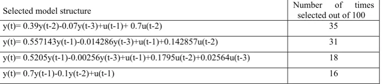
Table 2 Model selection results for Model II using the OLS-ERR algorithm

Selected model structure Number of times _{selected out of 100}

y(t)= 0.39y(t-2)-0.07y(t-3)+u(t-1)+ 0.7u(t-2) 35

y(t)= 0.557143y(t-1)-0.014286y(t-3)+u(t-1)+0.142857u(t-2) 31

y(t)= 0.5205y(t-1)-0.00256y(t-3)+u(t-1)+0.1795u(t-2)+0.02564u(t-3) 18

y(t)= 0.7y(t-1)-0.1y(t-2)+u(t-1) 16

Table 1 Model selection results for Model I using the OLS-ERR algorithm Parameter

Term True Estimate ERR(%)

y(t-1) -1.7 -1.704552 67.4213

u(t-1) 1.0 1.000453 28.0911

y(t-4) 0 -0.007688 2.9753

u(t-4) 0 0.008823 0.5170

y(t-3) 0 -0.020076 0.4823

u(t-3) 0 0.011086 0.1250

u(t-2) 0.8 0.801407 0.1524

y(t-2) -0.8 -0.815569 0.0342

process, even though noise free data were used. These results suggest that the low frequency AR(2) input process is so slowly varying that it is not sufficiently exciting for ARX or NARX model structure identification. An interesting phenomenon is that, although the 4 models given in Table 2 have different structures, they all produce the same (in fact indistinguishable) model predicted or long term outputs for any given input. Thus, in this regard, the four models are equivalent in output behaviour, even thought they are different in structure. It was also noticed that if the input signal was

set to a high frequency AR(2) process, say u(t)=0.6u(t-1)-0.0875u(t-2)+ξ(t)with )ξ(t)~N(0,1 , then

the true model structure will be correctly identified.

As noted earlier, many factors can affect model structure selection including the presence of noise, the sampling rate and the richness of the input signal. Some subjective factors such as the selected maximum lags in the input and output terms, and the nonlinear degree specified for nonlinear candidate model terms will also affect the model structure selection. It has been verified by numerous simulation examples that if the maximum lags or key variables of the system can be appropriately chosen, then most of the irrelative model terms can be excluded and confidence of correctly selecting a minimum model structure or nearly minimum model structure can be significantly increased. Thus determining suitable values for the maximum lags and selecting significant variables as a first stage in model structure selection is likely to be highly beneficial. Several algorithms are available for the determination of the maximum lags for both the input and the output (Bomberger and Seborg 1998, Feil et al. 2004, Wei et al. 2004). In many cases, however, suitable maximum lags and significant variables may be difficult to determine, and some alternatives are thus worthy of investigation.

3. The new IFOS algorithm

The above discussion suggests that there is a need to improve the OLS-ERR algorithm to try and ensure that the correct model structure can be determined even when the data sets are not ideal. This motivates the development of the new integrated forward orthogonal search (IFOS) algorithm assisted by both the squared correlation and mutual information criteria. Before describing the IFOS algorithm, some preliminaries will be described first.

3.1 Some definitions

Definition 1: Primary variables and derivative variables

A primary variable is a dependent variable that originally exists in the model which characterises a given system. A derivative variable is derived from the primary variables. Generally, a primary variable is explicit in the model, but a derivative variable is implicit.

Consider the model below

y(t)= f(y(t−1),y(t−2),u(t−1)) (12)

The variables here are the primary dependent variables. Iterating (12) by one

step with respect to the primary variable y(t-1), yields )

1 ( ), 2 ( ), 1

(t− y t− u t−

y(t)= f(y(t−1),y(t−2),u(t−1)) )) 1 ( ), 2 ( )), 2 ( ), 3 ( ), 2 ( ( ( − − − − −

= f f y t y t u t y t u t (13)

) 2 (t− y

The induced model (13) now involves 4 variables ,y(t−3), )u(t−1 and , where y(t-3)

and u(t-2) are derived variables. Inspection of the results in Table 1 for Model 1 in section 2.4 shows that some of the derived variables may have been induced by the presence of noise if the candidate maximum lags are set to be too high. Therefore, if the primary variables of the system can be determined initially from the observational data, the accuracy of the model structure selection can then be significantly improved. Notice that the non-uniqueness which produces the result that the models in Eqs. (12) and (13) are equivalent is in general a direct result of the discrete model form. This non-uniqueness is common in most discrete forms and is often independent of the structure selection algorithms employed.

) 2 (t− u

Definition 2: Model term dictionary

A model term dictionaryD is a set whose elements are some specified (candidate) model terms (also called atoms or bases in signal processing). A dictionary _D is said to be over-complete if all the true model terms are included in . A dictionary D D is said to be under-complete (or incomplete) if at least one true model term is not included in . A dictionary _{D D} is said to be exactly-complete if all the true model terms are included in , but D D contains no other candidate model terms. Clearly, for an

exactly-complete dictionary the identification problem reduces to a structure-known estimation problem. ) 1 ( ) 2 ( 1 . 0 ) 1 ( 7 . 0 )

(t = y t− − y t− +u t−

y

Assume that a system is described by the model: , then

), 1 (

{y t− y(t−1)u(t−1), u(t−2)} is over-complete; )} 2 ( ), 1 ( ), 2 ( ), 1 ( {

1= y t− y t− u t− u t−

D D₂ = is

under-complete; and D3 ={y(t−1),y(t−2),u(t−1)}is exactly-complete.

For a NARX model with a nonlinear degree land maximum lags (for output) and (for

input), the candidate model term dictionary, including the constant term, is y

n nu

} 0 , 0 , 1 , : ) ( ) (

{ 1 , 1 1

,

, l = x1 t Lxll t x ∈Vn n ≤ j≤l ≤ij≤l ≤i +L+i ≤l i

j i i

n

n y u

j u

y

D (14)

whereVny,nu ={y(t−1),L, y(t−n_y), u(t−1),_L, u(t−nu)}. The number of elements in the dictionary

is . C_lny+nu+l=[(n_y+n_u+_l)!]/[(n_y+n_u)!_l!]

l , , u y n n D

Definition 3: Model library

A model library_L is a set whose elements are some specified models. A model selection criterion is always performed over a given model library.

library are exactly correct but only approximately correct). What the ‘best’ model is, depends on the specific situation. For example, the first three models given in Table 2 are structure incorrect compared with the true model. However, all the four models are equivalent if the model predicted outputs are of the most concern. The ‘correctness’ of a model structure is thus always relative and the ultimate objective is always to find the model structure that best fits, in either the structure and the output behaviour, the real system under study.

Definition 4: Model behaviour equivalence

Two models and are said to be equivalent with each other in behaviour, if the (model

predicted) outputs of the two models, driven by the same input, are the same.

1

M M2

In practice, it may be impossible to get exactly the same output behaviour for two different

models. Thus, two models and are often considered approximately equivalent when their

outputs are sufficiently close when justified using a given criteria.

1

M M2

Assume that an identified model,_M , is given by

)) ( , ), 1 ( ), ( , ), 1 ( ( )

(t f y t y t n_y u t y t n_u

y = − _L − − _L − +e(t) (15)

At a given time instance , setting for k=1,2, …, , model predicted outputs

at time instances are defined as

) ( ) (

ˆ t₀ k y t₀ k

ympo _{− = −}

y n 0 t 0 t t≥ )) ( , ), 1 ( ), ( ˆ , ), 1 ( ˆ

(_ympo _{t y}mpo _{t ny u t u t nu}

f − _L − − _L −

=

) (

ˆ t

ympo _yˆmpo_{(t,M)= (16)}

While one-step-ahead predictions are often used to validate an identified model, previous experience shows that even a poor (e.g., insufficient, biased, unstable, etc.) model can provide good one-step-ahead predictions. Model predicted outputs can reveal severe model deficiencies which would otherwise go undetected by one-step-ahead predictions. However, in some cases, model predicted outputs may be unstable or may decay to zero, implying that model predicted outputs become invalid. In this case, a trade-off between one-step-ahead predictions and model predicted outputs is to use multi-step-ahead predictions.

3.2 Model term selection aided by mutual information

In the OLS-ERR algorithm described in section 2.2, a non-centralised squared correlation coefficient was used to measure the dependency between two vectors. This coefficient, between two vectors x and y, is defined as

∑

∑

∑

2 _{( )}

) )( ( ) ( ) , ( y y x x y x y

x (17)

3.2.1 Mutual information

Mutual information has now been extensively studied in the literature and applied to various areas. Following Cover and Thomas (1991), mutual information is defined as follows.

Consider two random discrete variables x and y with alphabet X andY, respectively, and with a

joint probability mass function p(x, y) and marginal probability mass functions and . The

mutual information is the relative entropy between the joint distribution and the product

distribution , given as

) (x

p p(y)

) , (x y

I

) ( ) (x p y p ⎟⎟ ⎠ ⎞ ⎜⎜ ⎝ ⎛ =

∑∑

x Xy Y

y

x (18)

The mutual information is the reduction in the uncertainty of y due to the knowledge of x, and

vice versa. Mutual information provides a measure of the amount of information that one variable shares with another one. If y is chosen to be the system output (the response), and x is one regressor in

a linear model, can be used to measure the coherence of x with y in the model. Several

algorithms have been proposed to estimate mutual information from observed data, see for example Moddemeijer (1989, 1999),

) , (x y

I

) , (x y

I

Darbellay and Vajda (1999), and Paninski (2003) and the references therein. In this study, the adaptive partitioning histogram method proposed in Darbellay and Vajda (1999) was employed to estimate relevant mutual information.

3.2.3 Inclusion of mutual information in model structure selection

Mutual information can easily be incorporated into the orthogonalization procedure in the same

way as the squared correlation coefficient. Let D ={φ_j:j=1≤ j≤M}be a given model term

dictionary. Let r0 =y, and

(19) )} , ( { max arg ₀ 1

1= _≤j≤M I r φj

l

where is the mutual information function given by (18). The first significant basis can thus be

selected as , and the first associated orthogonal basis can be chosen as . Set

) , (⋅⋅ I

1

1 φl

α = q₁=φ_l1

1 1 1 1 0 0 1 q q q q r r r _T T −

= (20)

In general, the mth significant model term can be chosen as follows. Assume that at the (m-1)th

step, a subset , consisting of (m-1) significant bases, , has been determined, and the

(m-1) selected bases have been transformed into a new group of orthogonal bases via

some orthogonal transformation. Let

1 2

1,α , ,αm−

α _L 1 − m D 1 2

1,q , ,qm−

q L 1 1 1 1 2 2 1 − − − − − −

− = − m

m T m m T m m m q q q q r r

∑

j _{q q} q

q

φ φ

q (22)

)} , ( { max

arg ( )

1 1 1 , m j m m k j m I k q r ₋ − ≤ ≤ ≠ = l

l (23) whereφ_j∈D−D_m−1. The mth significant basis can then be chosen as

m

m φl

α = and the mth associated

orthogonal basis can be chosen as . Subsequent significant bases can be selected in the same

way step by step.

) (m m qlm

q =

From (21), the vectors r_m−1and qm−1 are orthogonal, thus

1 1 2 1 2 2 2 2 1 ) ( || || || || − − − − − − = − m T m m T m m m q q q r r

r (24)

By respectively summing (21) and (24) for m from 2 to n+1, yields

n n m m m T m m T

m _{q r}

q q q r y

∑

1 ₍₂₅₎

∑

− − = n

m Tm m

m T m n 1 2 1 2

2 _{|| ||} ( )

|| || q q q r y

r (26)

The residual sum of squares, also called the sum-squared-error, , or its variants including the

mean-square-error (MSE) or the error-to-signal ratio defined as

2

|| ||r_n

2 2 _{|| ||}

||

||r_n y , can be used to form

criteria for model selection. The model term selection procedure can be terminated when some specified termination conditions are met.

The motivation for introducing the mutual information assisted criterion here is not to totally replace the commonly used ERR criterion, but rather to provide an alternative and complementary approach to the ERR criterion. Further details will be given in Section 4.

3.2.3 Parameter estimation

It is easy to verify that the relationship between the selected original bases , and the

associated orthogonal bases , is given by

m

α α α₁, ₂,_L,

m

q q q1, 2,L,

(27) m

m

m Q R

A =

where , is an matrix with orthogonal columns , and is an

unit upper triangular matrix whose entries

m

q q q₁, ₂,_L,

] , ,

[ 1 m

m α α

A = _L Qm N×m Rm

m

m× u_ij(1≤i≤ j≤m) are calculated during the

orthogonalization procedure. The unknown parameter vector, denoted by , for the

model with respect the original bases (similar to (4)), can be calculated from the triangular equation

with , where or .

T m m=[θ1,θ2,L,θ ]

θ

T m m=[g1,g2,L,g ]

g ( ₁ )/( T _k)

k k T k k

g = r ₋q q q ( )/( T _k) k k T k

g = y q q q

m m mθ g

R =

Note that some tricks can be used to avoid selecting strongly correlated model terms. Assume that

at the (m-1)th step, a subset , consisting of (m-1) significant bases, , has been

determined. Also assume that is strongly correlated with some bases in , that is,

1 2

1,α , ,αm−

α _L 1 − m D 1 − − ∈ _m

j D D

is a linear combination of . Thus there exist (m-1) real numbers , at least

one of which is different from zero, such that

1 2

1,α , ,αm−

α _L k1,k2,L,km−1

1 1 2

2 1

1 + + − −

= _{m m}

j kα k α k α

φ _L (28)

, such that From (27), there exists another set of real numbers, μ1,μ2,L,μm−1

1 1 2

2 1

1 + + − −

= _{m m}

j q q q

φ μ μ _Lμ (29)

For the candidate basis given by (29), equation (22) becomes

0 q q q q φ φ

q = −

∑

= 1 1 ) ( m k k k T k k T j j m

j (30)

Therefore, . In the IOFS algorithm, the candidate basis will be

automatically discarded if , where

0 )

( ( ) (m)₌

j T m

j q

q φ_j∈D−D_m

} , 1 { 10 )

(q(jm) Tq(jm)< −τ φTjφj τ is a positive number that is large enough. In this way, any severe multicolinearity or ill-conditioning can be avoided.

3.3 Model length determination

The role of model length determination in dynamical system identification has been widely recognised and various model selection criteria have been well established, see for example the recent review paper by Stoica and Selen (2004). Model selection criteria are often established on the basis of estimates of prediction errors, by inspecting how the identified model performs on future (never used) data sets. One general routine for model selection, which tries to avoid or reduce any possible bias introduced by relying on any particular test data sets, is cross validation (Stone 1974). Cross-validation has a number of variations, two commonly used variants of which are the leave-one-out (LOO), also called predicted sum of squares (PRESS) (Allen 1974), and generalised cross-validation (GCV) (Golub et al. 1979). Generalised cross-validation, due to its convenience of use and effectiveness for avoiding overfitting, has been widely accepted.

Following Golub et al. (1979) and Orr (1995), the generalised cross-validation criterion below will be used for model size determination

) MSE( ) GCV( 2 n n N N n ⎟ ⎠ ⎞ ⎜ ⎝ ⎛ −

= (31)

where N is the length of the training data set, n is the effective number of model terms (Moody 1992)

where GCV is a minimum value, and is the mean-square-error that is associated to

the model of n model terms. It should be pointed out that the GCV criterion tends to produce

overfitted models (Friedman and Silverman 1989, Barron and Xiao 1991). The evaluation of the performance of the GCV criterion and some relative improvements have been reported in Billings and Wei (2007a).

N n) || _n|| /

MSE( _{= r} 2

Statistical methods play a unique role in the diagnosis and analysis of linear models. One aspect of the application of statistical methods for linear model analysis is hypothesis testing on regression coefficients (Hocking 1976, 1983, Montgomery et al. 2001). Consider the linear regression model with k regressors below

e

Xθ

y= + (32)

where y is , X is (if a constant term is included in (32), then all the elements of the first

column of X are assumed to be unit), θis 1

×

N N×n

, e is 1

×

n n×1, and n=k+1. Equation (32) is equivalent to (5), where y and X in (32) can be viewed as the output vector and the associated regression matrix A

in (5), respectively. A frequently asked question is: do all the k regressors contribute significantly to the regression model?

The simplest but useful hypothesis for testing the significance of any individual regression

coefficient, for instance θ_j in the model (32), is

0 :

0 θj =

H (33a) 0

:

1 θj ≠

H (33b)

0 :

0 θj =

H

If there is no sufficient reason to reject the null hypothesis , then the corresponding

regressorx_jcan be removed from the model. The test statistic for this hypothesis is

) ˆ se( | ˆ | 0 j j t θ θ

= (34)

* 2

ˆ ) ˆ

se(θ_j = σ c_jj

where is the standard error of the regression coefficient , is the diagonal

element of corresponding to , and is the unbiased

estimator of variance.

* jj c j θ j θˆ 1 )

(XTX − _=yT_{(I−H)y/(N−n)}

s

MS_Re 2

ˆ =

σ

For a givenα, if t0 >tα/2,_N−_n, the null hypothesisH0:θj =0 can then be rejected. Note that this is

really a partial or marginal test (Montgomery et al. 2001) because the regression coefficient

depends on all of the other regressors that are in the model. Thus it is a test of the contribution of

given the other regressors in the model. j θˆ j x 96 . 1 , 2 / N−n≈

tα α

, if

For practical identification problems, where N−n>120 is set to 0.05, an

equivalent test to (34) is

) ˆ se( 96 . 1 | ˆ | 0 j j t θ θ

= (35)

If , the null hypothesis can then be rejected at the 95% confidence interval. Detailed

information for the explanation of the rationale and the theoretical derivations for the above statistic can be found in (Montgomery et al. 2001).

0 :

0 θj =

H

1

0> t

procedure, where significant model terms are selected step by step, one at a time. This procedure, coupled with the GCV criterion, will produce a model (or a set of models) formed by the selected significant model terms. But it has been noted that some spurious model terms may still be in the resultant model when the input is poorly designed. To refine the resultant model, the t-test is then used to detect and then remove the most probable spurious model terms.

In the next section, illustrations will be presented to show how the proposed IFOS algorithm works. A general procedure and some recommendation on how to apply the IFOS algorithm will then be given in Section 5. In the following, the IFOS algorithm, aided by the squared correlation, will be referred to as IFOS-SC. Similarly, the algorithm aided by mutual information criterion, will be referred to as IFOS-MI. As will be seen, for the same identification problem, IFOS-SC and IFOS-MI may or may not produce exactly the same model structure. By evaluating the performance of the resulting models, in accordance with some specified measures, a more accurate model structure can often be obtained. The relationship between ERR and MI criteria have not yet been found (Billings and Wei 2007b). A further study is still needed to reveal conditions under which one algorithm outperforms the other.

4. Case studies

In this section, several examples are provided to illustrate how to select an accurate model structure using the new IFOS algorithm. It will be shown that the IFOS algorithm can detect spurious model terms even when the data are contaminated with noise. A spurious model term here means that the model term is not in the true model but is selected with an ERR value that is not small. For cases where the input may not be sufficiently exciting, a trial-and-error approach can be used to avoid selecting the terms y(t-1), y(t-2), etc., since these terms are most likely to be selected even if they are not in the true model. In cases where the true model is not known, the performance of model predicted outputs will be examined to find the best model from a model set containing several candidate models generated from different libraries.

Notice that in the given examples, both artificial models and real data sets, where it is believed to be difficult to find the correct model structure, have been deliberately chosen to illustrate the effectiveness of the new IFOS algorithm. The examples are therefore far more demanding than typical model structure selection problems.

4.1 Example 1—the input is white

The following model was taken from Mao and Billings (1997)

) 2 ( 6 .

0 2 ₋

+ u t

) 2 ( 5 . 0 )

(t =− y t−

y +0.7y(t−1)u(t−1) )

1 ( 2 .

0 3 ₋

Table 3 Identified model structure for system (36) using the IFOS-SC algorithm Parameter

Term True Estimate ERR(%) t-test GCV

y(t-1)u2_{(t-2) 0 0.014704 34.9921 0.7382 0.074273}

y(t-1)u(t-1) 0.7 0.706678 21.9095 69.9612 0.049441

u2_{(t-2) 0.6 0.601460 12.3828 99.9614 0.035379}

y(t-2) -0.5 -0.491838 23.6688 59.4477 0.008150

y3_{(t-1) 0.2 0.204638 4.5382 33.6203 0.002915}

y(t-2)u2_{(t-2) -0.7 -0.708220 2.1595 27.4588 0.000412}

y(t-1)u(t-4) 0 -0.026297 0.0045 1.1833 0.000403

y2_{(t-2)u(t-3) 0 -0.012915 0.0044 1.1315 0.000400}

y(t-4)u(t-2) 0 0.017330 0.0043 1.6214 0.000396

y(t-3)y(t-4)u(t-2) 0 -0.025846 0.0032 1.1110 0.000397

Run time: 0.906s

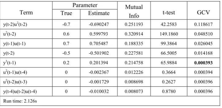
Table 4 Identified model structure for system (36) using the IFOS-MI algorithm Parameter

Term True Estimate Mutual _Info t-test GCV

y(t-2)u2_{(t-2) -0.7 -0.690247 0.251193 42.2583 0.118617}

u2_{(t-2) 0.6 0.599793 0.320914 149.1860 0.048510}

y(t-1)u(t-1) 0.7 0.705487 0.188335 99.3864 0.026045

y(t-2) -0.5 -0.501902 0.227581 66.5005 0.014168

y3_{(t-1) 0.2 0.201394 0.214758 65.9884 0.000393}

u2_{(t-1)u(t-4) 0 -0.002367 0.012226 0.3664 0.000394}

u2_{(t-2)u(t-3) 0 -0.001729 0.008698 0.2627 0.000396}

y(t-4)u(t-2)u(t-4) 0 -0.010032 0.008073 0.8780 0.000396

Run time: 2.126s

where the input u(t) was uniformly distributed on [-1, 1], with the noise e . Following

Mao and Billings (1997), the maximum lags of both the input and the output were assumed to be 4 and the nonlinear degree to be 3. Five hundred input-output data were generated and were used for model structure selection. The new IFOS algorithm, which incorporates the t-test given by (35), was applied to the data set, and the results are shown in Tables 3 and 4.

) 02 . 0 , 0 ( ~ )

(t N 2

From Table 3, the ERR values show that the first 6 model terms are significant and should be included in the model. The first selected term, y(t-1)u2_{(t-2), with the highest ERR value is spurious.}

values show that the appropriate number of model terms is 9, but clearly a model of 9 terms is overfitted.

Compared with Table 3, results given in Table 4 are quite optimistic. The t-tests show that only 5 model terms are significant, and the five model terms are exactly consistent with the 5 true model terms. In addition, GCV provides a correct indication of the structure, suggesting that 5 model terms are appropriate. Thus, from the results given by Table 3 and 4, all model terms can be correctly determined.

4.2 Example 2—the input is non-white

Consider the following two systems

5 . 0 ) 2 ( 05 . 0 ) 1 ( 2

2 _{− − − +}

+u t w t

) 2 ( 8 . 0 ) 1 ( 5 . 0 )

(t = wt− + u t−

w

: (37a)

1 S ) ( 5 . 0 1 1 ) ( )

( ₁ t

q t

w t

y ₋ ξ

− +

= , (37b) _ξ(_t)~_N(0,0.052)

) 1 ( 3 . 0 ) 2 ( ) 1 (

25 _{− − −} 3 ₋

+ u t u t u t

) 2 ( 5 . 0 ) 1 ( )

(t =u t− + u t−

w

: (38a)

2 S ) ( 8 . 0 1 1 ) ( )

( ₁ t

q t

w t

y ₋ ξ

− +

= , (38b) _ξ(_t)~_N(0,0.022)

Following Piroddi and Spinelli (2003), the input u(t) to the two systems were chosen as a low frequency AR(2) process of the form: u(t)=1.6u(t-1)-0.6375u(t-2)+0.16ζ(t), with ζ(t)~N(0,1). Two

data sets of 500 input-output samples were generated from each system and the two data sets were used for model structure selection.

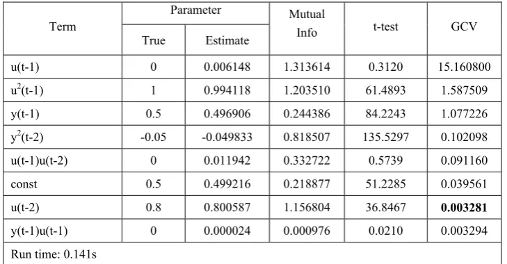
4.2.1 Experiments for system S₁

Following Piroddi and Spinelli (2003), the maximum lags of both the input and the output were assumed to be 2 and the degree of nonlinearity to be 2. Model structure selection results for system are reported in Tables 5 and 6. Following the analysis in Example 1, it is clear that the significant

model terms should be selected as y(t-1), u(t-2), u

1

S

2_{(t-1), y (t-2), and the} 2 _{const term, which are exactly}

the same as the true model. Note that once the 5 model terms have been determined, the parameters need to be re-estimated based on just these selected model terms.

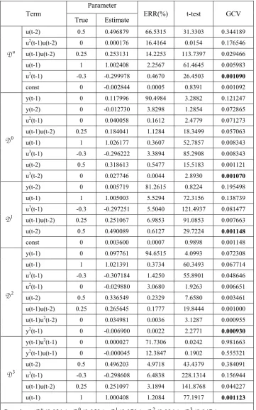
4.2.2 Experiments for system S₂

Following Piroddi and Spinelli (2003), the maximum lags of both the input and the output were assumed to be 2 and the degree of nonlinearity to be 3. To ensure selection of the correct model subset, the IFOS-SC algorithm was applied over the following 5 different candidate model term dictionaries: 3 , 2 , 0 D

Du = , _D0_=D2,2,3, )} 1 ( {

0

1_{=D − y t−}

D , )} 2 ( { 0

2_{=D − y t−}

)} 2 ( ), 1 ( {

0

3_{=D − y t− y t−}

D ,

where the model term dictionary D was defined by (14). The reason that the 5 different

candidate dictionaries were considered here was two fold: one goal is to illustrate that the choice of initial dictionaries will affect the model selection results, and another goal is to show that spurious model terms can be detected using the t-test. Five different models, corresponding to the 5 dictionaries, were selected and the identified models are shown in Table 7. Similar results were also obtained using the IFOS-MI algorithm, but are not shown to save space.

l

, , u y n

n

While it is not quite apparent which model terms should be included in the model from the results

with respect to D and D , it is quite clear from the results with regard to D , D and D that the significant model terms included in the model should be u(t-1), u(t-2), u(t-1)u(t-2), and u

u

0 2 1 3

3_{(t-1), which}

are exactly the same as required by the system. Note that the search time to select the model terms is quite short, and it is less than 0.1s for each of the 5 cases.

Table 5 Identified model structure for the system (37) using the IFOS-SC algorithm Parameter

Term

True Estimate ERR(%) t-test GCV

y(t-1) 0.5 0.500106 91.1027 71.4985 1.511037

y2_{(t-2) -0.05 -0.049757 3.5098 128.3416 0.922388}

u2_{(t-1) 1 1.000401 2.0742 132.8120 0.571884}

u(t-2) 0.8 0.806721 2.8537 125.5270 0.079973

const 0.5 0.493459 0.4406 43.4106 0.003336

y2_{(t-1) 0 -0.000419 0.0001 0.8359 0.003343}

u2_{(t-2) 0 0.006367 0.0001 0.6223 0.003360}

Run time: 0.032s

Table 6 Identified model structure for the system (37) using the IFOS-MI algorithm Parameter

Term

True Estimate

Mutual

Info t-test GCV

u(t-1) 0 0.006148 1.313614 0.3120 15.160800

u2_{(t-1) 1 0.994118 1.203510 61.4893 1.587509}

y(t-1) 0.5 0.496906 0.244386 84.2243 1.077226

y2_{(t-2) -0.05 -0.049833 0.818507 135.5297 0.102098}

u(t-1)u(t-2) 0 0.011942 0.332722 0.5739 0.091160

const 0.5 0.499216 0.218877 51.2285 0.039561

u(t-2) 0.8 0.800587 1.156804 36.8467 0.003281

y(t-1)u(t-1) 0 0.000024 0.000976 0.0210 0.003294

Table 7 Identified model structures for the system (38) using the IFOS-SC algorithm Parameter

Term

True Estimate ERR(%) t-test GCV

u(t-2) 0.5 0.496879 66.5315 31.3303 0.344189

u2(t-1)u(t-2) 0 0.000176 16.4164 0.0154 0.176546

u(t-1)u(t-2) 0.25 0.253131 14.2253 113.7397 0.029466

u(t-1) 1 1.002408 2.2567 61.4645 0.005983

u3_{(t-1) -0.3 -0.299978 0.4670 26.4503 0.001090}

u D

const 0 -0.002844 0.0005 0.8391 0.001092

y(t-1) 0 0.117996 90.4984 3.2882 0.121247

y(t-2) 0 -0.012730 3.8298 1.2854 0.072865

u2_{(t-1) 0 0.040058 0.1612 2.4779 0.071273}

u(t-1)u(t-2) 0.25 0.184041 1.1284 18.3499 0.057063

u(t-1) 1 1.026177 0.3607 52.7857 0.008343

u3_{(t-1) -0.3 -0.296222 3.3894 85.2908 0.008343}

u(t-2) 0.5 0.318613 0.5477 15.5183 0.001121

0

D

u3_{(t-2) 0 0.027746 0.0044 2.8930 0.001070}

y(t-2) 0 0.005719 81.2615 0.8224 0.195498

u(t-1) 1 1.005003 5.5294 72.3156 0.138739

u3_{(t-1) -0.3 -0.297251 5.5040 121.4937 0.081477}

u(t-1)u(t-2) 0.25 0.251067 6.9853 91.0853 0.007663

u(t-2) 0.5 0.490089 0.6127 29.7224 0.001148

1

D

const 0 0.003600 0.0007 0.9898 0.001148

y(t-1) 0 0.097761 94.6515 4.0993 0.072308

u(t-1) 1 1.021391 0.3734 60.3493 0.067714

u3_{(t-1) -0.3 -0.307184 1.4250 55.8901 0.048646}

u2_{(t-1) 0 -0.029880 3.0680 1.9263 0.006651}

u(t-2) 0.5 0.336549 0.2329 7.6580 0.003461

u(t-1)u(t-2) 0.25 0.265645 0.1777 19.8444 0.001000

u(t-1)u2_{(t-2) 0 0.034981 0.0036 3.1287 0.000955}

2

D

y2_{(t-1) 0 -0.006900 0.0022 2.2771 0.000930}

y(t-1)u2_{(t-1) 0 0.000027 71.7306 0.0242 0.981663}

y2_{(t-1)u(t-1) 0 -0.000045 12.3847 0.1902 0.555321}

u(t-2) 0.5 0.496203 4.9718 43.4379 0.384091

u3_{(t-1) -0.3 -0.298608 6.4838 228.1314 0.156944}

u(t-1)u(t-2) 0.25 0.251097 3.1894 141.8768 0.044227

3

D

u(t-1) 1 1.000408 1.2084 77.1917 0.001123

4.3 Example 3—forecasting annual sunspot numbers

The data set used in this example contains 301 observations of the annual sunspot numbers from 1700 to 2000. The first 280 samples for years 1700 to 1979 were used for model identification and the remaining 22 data were used for model performance testing. The candidate model term dictionaries

were chosen as 0 _12,0,1

D

D = ={y(t−1),_L, y(t−12)}, and -{y(t-1),y(t-2)}. The reason that the

maximum lag was chosen to be 12 is due to the fact that the annual sunspot time series has a cycle that is about 11years. Although a nonlinear model for the sunspot time series may be more appropriate, the objective in this example is to illustrate the efficiency of the new IFOS algorithm for model structure selection, and a linear model was thus adopted.

0 1

D

D =

The selected model structures from the dictionary using both IFOS-SC and IFOS-MI are shown in Table 8. Both algorithms suggested that the best model subset be chosen as {y(t-1), y(t-2), y(t-9),

const}. The selected model structures from the dictionary by both IFOS-SC and IFOS-MI required

5 model terms: y(t-3), y(t-4), y(t-9), y(t-11), and const. It easily be shown that the performance of the

model generated from is much inferior compared with the model generated from .

0

D

1

D

1

D D0

The fact that the two different criteria (squared correlation and mutual information) yield the same results indicates that the linear regression model is dominated by the three significant variables y(t-1),

y(t-2) and y(t-9). This result enhances the previous conclusion (Wei et al. 2004) that y(t-1), y(t-2) and

y(t-9) are the three most important variables for describing the sunspot time series over the period from 1700 to 1979. By re-estimating the parameters in a linear model, the final identified model was

given by y(t)=6.0223+1.2352y(t-1)-0.5404y(t-2)+0.1917y(t-9). One-step-ahead predictions and model

predicted outputs produced by the identified model over the test data set are shown in Figure 1.

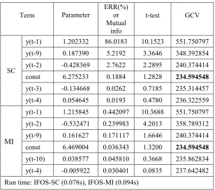
Table 8 Identified model structures for the sunspot time series ERR(%)

Term Parameter or Mutual

info

t-test GCV

y(t-1) 1.202332 86.0183 10.1523 551.750797 y(t-9) 0.187390 5.2192 3.3646 348.392854 y(t-2) -0.428369 2.7622 2.2895 240.374414 const 6.275233 0.1884 1.2828 234.594548 SC

y(t-3) -0.134668 0.0262 0.7185 235.314457 y(t-4) 0.054645 0.0193 0.4780 236.322559 y(t-1) 1.215845 0.442097 10.3688 551.750797 y(t-2) -0.532471 0.239983 4.2013 358.789312 y(t-9) 0.161627 0.171117 1.6646 240.374414 const 6.469004 0.036343 1.3200 234.594548

MI

y(t-10) 0.038577 0.045810 0.3668 235.862834 y(t-4) -0.005922 0.030401 0.0835 237.642482 Run time: IFOS-SC (0.078s), IFOS-MI (0.094s)

4.4 Example 4—Drosphila or fruit fly modelling

This data set came from experiments and observations on a fruit fly, called Drosophila. The system input was the response of the photoreceptors, and the output was the response of the large monopolar cells. Recordings of 1000 points, sampled at a rate of 1kHz, on wild-type flies were collected.

The relationship between the input and the output in the fruit fly experiment is complex, because in addition to the response from the photoreceptors, several other factors may also affect the output response of the large monopolar cells. Identification of models relating these responses is therefore quite challenging. The objective of this example is to find a model that reflects, as closely as possible, the relationship between the response of the photoreceptors (the input) and the response of the large monopolar cells (the output), to facilitate the analysis and understanding of the associate behaviour of this kind of insect.

The maximum lag for the input and the output were chosen to be 5 and 3, respectively, and the degree of nonlinearity to be 3. Similar to previous examples, the following 6 candidate model term dictionaries will be considered:

5 , 3 , 0

D

Du = , , , , _D1_=D0₋{_y(_t−1)} _D2 _=D0_{−{y(t−2)}} 3

, 5 , 3 0

D

D =

)} 2 ( ), 1 ( {

0

3 _{=D − y t− y t−}

D , _D4_=D0₋{_y(_t−1),_y(_t−2),_y(_t−3)},

where the set was defined as defined as ={y(t-1), …, y(t- ), u(t), u(t-1), …, u(t- )}. The

reason that the 6 different candidate dictionaries were considered here was as follows. Experience has shown that the terms y(t-1), y(t-2), etc. are most likely to be selected even if they are not in the true model. Based on this observation, the 6 different initial dictionaries were considered and these led to 6 different models. The model that produces the best output performance was chosen to be the final model. The average time used by the IFOS-SC algorithm for model structure selection, over different model term dictionaries, was 2.425s, and 4.688s for the IFOS-MI algorithm running on a standard PC.

y

n

u y n

n

V _,

u y n

n

V _, n_u

Following the same procedures as described in previous examples, the IFOS-MI identified model,

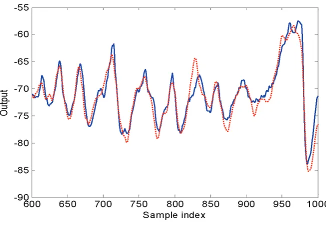
selected over the dictionary , was found to be the best model, because the performance of the long-term predictions produced by this model were superior to the other identified models. The final IFOS-MI identified model contained 10 model terms. A comparison between the model predicted outputs and the measurements over the validation data set is shown in Figure 3. Clearly, the identified model fitted the experimental data extremely well.

2

D

Fig. 3. A comparison between model predicted outputs and the measurements over the validation data set the fruit fly modeling problem. Solid line indicates the measurements and the dashed line indicates the model predicted outputs from the identified model for the fruit fly data set.

5. Discussions and recommendations

Model structure selection is a central issue in any nonlinear system identification problem. In addition to the input signal and sampling interval, many other factors, including the initial choice of the maximum lags for both the input and the output, the determination of the primary variables, the choice of initial candidate model term dictionaries, and the presence of noise (uncertainty in the data), all affect model structure selection. All these are generic problems in nonlinear system identification.

It is known that if the maximum lags or key (primary) variables for the system can be appropriately determined in advance, then irrelevant model terms can be precluded. Thus determining suitable maximum lags and selecting significant variables is a key step that could greatly improve the accuracy of all model structure selection procedures.