Solution of a Second Order Elliptic Partial Differential Equation with Varying Complex Coefficients: An Application for Computing Effective Complex Electrical Properties of Materials represented by 3D Images

(1)

Solution of a Second Order Elliptic

Partial Differential Equation with

Varying Complex Coefficients: An

Application for Computing

Effective Complex Electrical

Properties of Materials represented

by 3D Images

Johnny Valbuena Soler

A thesis submitted for the degree of

Doctor of Philosophy

(2)

Except where otherwise indicated, this thesis is my own original work.

Johnny Valbuena Soler October 23, 2017

To the memory of my beloved and adorable mother, Maria.

c

(3)

Acknowledgments

First and foremost, I would like to express my deepest and most heartfelt gratitude to Prof Wolfgang Hackbusch for believing in me and offering me his continuous sup-port and dedication. Without his guidance, his expertise and his persistent help, I would still be "lost" in my research. I could not imagine having a better supervisor and advisor than Prof Hackbusch, whose passion for mathematics is utterly conta-gious. We spent many long hours on the whiteboard and his personal enthusiasm kept me engaged with my research and gave me the necessary encouragement to keep going. I am also very grateful to his beloved wife, Mrs. Ingrid for welcoming me in their home in Kiel, Germany, and preparing some delicious meals for us, while we were discussing numerical applications.

I would also like to thank Prof Tim Senden and specially Prof Adrian Sheppard, the chair of my supervisory panel, for not giving up on me and for their assistance and generous support along my long journey.

A very special thank you goes to Prof. Steffen Börm, Chair of Scientific Comput-ing at the University of Kiel for all his help and unconditional support in makComput-ing my multiple stays in Kiel comfortable and affordable, but also for always keeping a door open when I needed to unwind and talk about ideas for my future career. I would also like to thank Prof Börm ’s group: Linda, Nadine, Sven, Jens, and Dirk.

I express my sincere thanks to Dr. Ronald Kriemann for all his support to use and install theH-LibProlibrary, and the discussion of the convergence results.

My appreciation also extends to Mrs Ritter, the administrative assistant at the University of Kiel Guest House, for her constant help in finding accommodation for me and assisting me in my non-existent knowledge of the German language.

I would not have reached the last stage of the PhD process without the adminis-trative constant support and help from Mrs. Luidmila Mangos (Luda). Many thanks for everything you have done to assist me in submitting my PhD.

I am also forever grateful to my dear friend Tony Karrys, who was always very supportive and a true friend through the many years I stayed in University House. His sense of humour and his immense heart kept me going through the difficult times that one can endure when doing a PhD.

This acknowledgement would not be complete if I did not express my utmost and heartfelt thanks to my very dear friend Amalia. With her constant generous support and her true friendship, she made my road much less rugged. I would also like to thank my friends Babu, Alon, David, Jill, Vivian, Nicolas, Marion and my little friend Nonoshe for their constant support, their humour and their friendship.

Finally, I would like to thank my partner Eleonora, for her incredible patience, her love and her unconditional support in this valuable experience of my life.

(4)

Abstract

Materials may be characterised by using their electrical properties which establish how they interact when an electric field is applied at various frequency ranges. This interaction is used to determine properties of materials such as moisture content, bulk density, bio-content, chemical concentration and stress-strain. In the case of the physical characteristics of rocks, the response of the minerals under the influence of an electric field is different at distinct frequencies due to their chemical compounds. It affects the electrical properties.

The computing of complex effective permittivity and complex effective conductiv-ity of materials plays an important role due to its applications in different fields. The response of these properties under the influence of an alternating current field is used to characterise materials. The development of an approach to calculate these proper-ties involves the solution of the second order elliptic partial differential equation as ∇ ·[Q(ω)∇u(x,y,z)] =0, whereQ(ω)∈C3×3represents the physical parameters of the different phases in the material, andu(x,y,z)is the electric potential. The main difficulty in solving this equation comes from the high contrast of the coefficients in the distinct phases of the material.

There is an efficient approach that is used to compute the effective electrical con-ductivity of material under the influence of a static field. The material is represented in a 3D image. The Finite Element method and periodic boundary conditions are used to build an energy function which is minimised using the Conjugate Gradient algorithm. It allows to obtain the electric potentials, and then the computation of the conductivity is carried out. Moreover, this approach can also be used to calcu-late effective permittivity of material when a static field is applied, just by making a few changes in the approach. However, it is not possible to modify this approach to compute complex effective permittivity and complex effective conductivity because if one wants to obtain the electric potentials, a complex energy function has to be minimised.

This research is focused on developing a numerical scheme that allows to solve the second order elliptic partial differential equation with varying complex coeffi-cients in order to obtain the electrical potentials. In the initial stage, a few tools of functional analysis are used to transfer the strong formulation into the variational or weak formulation in the appropriate functional space. A demonstration is made to prove that the sesquilinear form is bounded andV-elliptic. These conditions are necessary to use the Lax-Milgram theorem which guarantees that there is a solution, and that it is unique. In order to find the best approximation uh to the solution u

of the variational problem, the Galerkin method and the orthogonality condition be-tween u anduh are used to produce the bestuh in a given approximating subspace

(5)

in a finite-dimensional space. The process of construction of the finite-dimensional subspace is carried out using the Finite Element method.

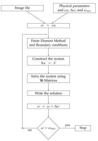
The first stage of the numerical scheme consists in constructing a complex system of linear equations that arises from the second order elliptic partial differential equa-tion. This is carried out by using the physical parameters of the material represented in a 3D image, the frequency where an electric field is applied, the employment of the Finite Element method, and the application of the Dirichlet and the Neumann boundary conditions. The second phase in the numerical scheme focuses on solving the complex system. The solution is computed using the technique of Hierarchical Matrices in combination with a Linear Method and the Generalised Minimal Resid-ual Method algorithm. A C code was written to implement the scheme. The code uses the NetCDF library to read the 3D image and theH-LibProlibrary to work with the Hierarchical Matrices.

(6)

Notation

k · k_Y←X norm of a mapping (matrix) fromX intoY (·,·),(·,·)_0,_Ω,(·,·)_L2₍₍_Ω₎ scalar product

h·,·i scalar product h·,·i_V_×_V0 duality form

k · k2 Euclidean norm

∆ gradient

⊕_r formatted matrix addition with truncation to rankr

formatted matrix-matrix multiplication •|_b,•|τ×σ restriction of a matrix to a blockbor τ×σ

η factor in admissibility condition #S cardinality of a setS

α,β,γ indices of the index set

εij dielectric constant in the directioni= j={x,y,z}

ε0 dielectrci constant of air ρ(M) spectral radius of a matrix M τ, σ symbols representing clusters

ω frequency

Γ the boundary of theΩ

ΓD Dirichlet boundary condition

ΓN Neumann boundary condition

Φ(u,b,L) function describing an iteration

Ω an open set inRnor a domain

Ωh a grid

a(·,·) sesquilinear form

Aαβ, aαβ, Aij,aij entries of the matrixA

V_mH₊₁ Hermitian transport matrix

C complex numbers

CI _{complex space of the vectors corresponding to the index set} _I CI×I _{complex space of the matrices corresponding to the index set} _I

D(Φ) domain of the iterationΦ

em errorxm−xof themth iterate

f vector

fi entries of the vectorf

G(A) graph of the matrix A

H1(Ω), H₀1(Ω),H_Γ1_D(Ω) Sobolev Spaces

h step size

H_p matrix model format

(7)

Contents vii

H(r,P) set of hierarchical matrices

i,j,k indices of the ordered index set

I identity matrix

I index set

Iα subset of block indeces

I,J,K index sets

Init(Φ,L) cost for initialising the iterationΦ Km(X,v) Krylov space

L(X,Y) linear space of bounded operators fromXtoY L2(Ω) space of square-integrable functions

L the stiffness matrix

Lij entries of the stiffness matrix

L matrix

L set of consistent linear iteration L(T(I)) set of leaves of the clusterT(I)

M matrix

N matrix

N natural numbers{1, 2, 3,· · · }

N0 N∪ {0}={0, 1, 2, 3,· · · }

P partition of a hierarchical matrix

P+, P− far field, near field

Q 3×3 complex parameter matrix

Qmin bounding box

R(r,I), Rr set of rank-rmatrices

R real numbers

span{· · · } linear space spanned by{· · · }

supp(·) support of a function

ST(τ) set of sons ofτ∈ T

T_rR_←_s truncation of a rank-smatrix to rank-r

T_rR truncation to rankr

T(I) cluster tree belonging to the index setI T(I×I) block cluster tree for I×I

un a grid function

Vh finite element space

Work(Φ,L) amount of work of the iterationΦapplied to Lu=b xm _m-_th_iterate

Xτ support of the clusterτ

y vector

(8)

List of Figures

1.1.1 The textural model filled with water and oil (left). The representa-tion of the textural model with random distriburepresenta-tion of oblate ellip-soids(right). Image after Abdullah et al. [2007] . . . 3

1.1.2 (a) Real well sorted media. (b) Real poorly sorted media. Image after Boggs [20011]. . . 4

3.2.1 (a) A porous material. (b) Discretisation of the porous material(cont.) . 35

3.2.1 (c). The grid points of the discretisation where the active points are represented by the black circles and the boundary points are illustrated by the red circles. . . 36

3.4.1 The construction process of the complex linear system for each fre-quency within a range using a 3D image, the physical properties of the material, Finite Element method and the boundary conditions. The complex linear systems are solved by using H-Matrices. . . 42

5.2.1 SupportsXτ andXσ. Image after Hackbusch [2015]. . . 56

5.4.1 Block partitions. Image after Hackbusch [2015]. . . 60

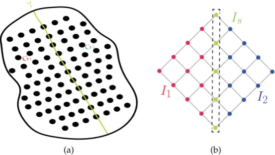
5.5.1 (a) The graphs G1 andG2 and the separator γ. (b) The graphs repre-sented in the graph matrix. . . 69

5.5.2 The two level recursion: (a) The subgraphsG3,G4,G5, andG6, and the separators γ, γ1, and γ2. (b) The graph matrix of the subgraphs. (c) The corresponding block matrices of theH-matrix. . . 70 5.5.3 The factorLwhere the white colour represents the zero blocks. Image

after Hackbusch [2016]. . . 72

6.2.1 The convergence behaviour of the solutions of the complex systems of linear equations generated by the interval of frequencies from the sphere sample is plotted vs the frequency. Only one H-LU decom-position at the first frequency is computed and it is used to solve all complex systems. . . 78

(12)

xii LIST OF FIGURES

6.2.2 (a) The convergence of the solutions of the complex systems of equa-tions from the sphere sample is plotted vs the frequency. The differ-ent subintervals are represdiffer-ented by distinct colours. The lowest peaks of convergence rate in each subinterval correspond to the frequency where the H-LU decomposition is computed. For the rest of the fre-quencies in each subinterval, its corresponding H-LU decomposition is used to solve the complex systems of equations. (b) The convergence rate vs frequency are plotted for three subintervals of frequency. . . 80 6.2.3 The convergence behaviour of the solutions of the complex systems

of linear equations generated by the interval of frequencies from the random voxel sample is plotted vs the frequency. Only one H-LU

decomposition at the first frequency is computed and it is used to solve all complex systems. . . 81 6.2.4 (a) The convergence of the solutions of the complex systems of

equa-tions from the random voxel sample is plotted vs the frequency. The different subintervals are represented by distinct colours. The lowest peaks of convergence rate in each subinterval correspond to the fre-quency where the H-LU decomposition is computed. For the rest of the frequencies in each subinterval, its corresponding H-LU decom-position is used to solve the complex systems of equations. (b) The convergence rate vs the frequency are plotted for three subintervals of frequency. . . 83 6.2.5 (a) The convergence iteration of the solutions of the complex systems

of equations from the sphere crystal sample is plotted vs the frequency. The different colours represent distinct subintervals of frequency. The lowest peaks of convergence rate in each subinterval are associated to the frequency where the H-LU decomposition is calculated. For the rest of frequencies in each subinterval, its corresponding H-LU

decomposition is used to solve the complex systems of equations. (b) The different convergence rates are computed in the first subinterval using three accuracy values. . . 86 6.2.6 The convergence speed vs the frequency are plotted for three

subinter-vals of frequency. . . 87 6.3.1 (a) The convergence of the solutions of the complex systems of

(13)

LIST OF FIGURES xiii

6.3.2 (a) The convergence of the solutions of the complex systems of equa-tions from the Bentheimer sample is plotted vs the frequency. The different subintervals are represented by distinct colours. The lowest peaks of convergence rate in each subinterval correspond to the fre-quency where the H-LU decomposition is computed. For the rest of the frequencies in each subinterval, its corresponding H-LU decom-position is used to solve the complex systems of equations. (b) The convergence rate vs the frequency are plotted for three subintervals of frequency. . . 91 6.3.3 (a) The convergence of the solutions of the complex systems of

(14)

(15)

Chapter1

Introduction

The development of materials has an incalculable impact on our daily life. This is im-portant for different industries such as aerospace, automotive, biological, chemical, electronic, energy, metals, and telecommunications. Each major technology is under-lain by understanding the behaviour and properties of materials. When materials are exposed to external stimuli, they generate some type of response. The properties of materials can be measured in terms of the kind of response and its magnitude under the influence of a specific stimuli.

The response of a material under the application of a magnetic field shows the magnetic properties. When light or electromagnetic radiation is used as a stimulus, the optical properties are represented by an index of refraction and reflectivity. The capacity and thermal conductivity are properties of solids that describe their thermal behaviour. The electrical properties such as electrical conductivity and dielectric constant can be measured when an electric field is used as a stimulus. The elastic modulus, strength and toughness are mechanical properties which are related to the deformation of materials when load or force is applied to them.

The analysis of 3D digital images of materials has become the most popular tool to generate information about their structures and properties. A virtual material laboratory to study real complex material was developed by a group of researchers in the Applied Mathematics Department at the Australian National University. Even though their focus is on oil and gas applications, the scheme developed by them is also used to characterise materials in general. Basically, the scheme has four steps: data exploration is the first step and it consists in identifying the configuration of the phases or components in the material using computer visualisation. The second step is the data segmentation which classifies the information in each voxel of the image according to an assumption and a single grayscale image. The representation of the phases in the voxels is very important to quantify the physical properties from the image. The morphological and geometrical analysis is the third step; it produces information about how the different phases are connected and how is their geometrical structures are. The last step is the numerical analysis, that comes as a results of applying the first three steps; the phases, pore, and grains in the materials are represented in different portions in the image. Then, the physical properties are computed assigning the constituent material properties, and solving the adequate equation under suitable boundary conditions [Sakellariou et al., 2007].

(16)

2 Introduction

Computational rock physics is an approach defined by a group of researchers in the School of Earth Science, Energy, and Environmental Sciences at Stanford Univer-sity. The approach is based on imaging rock to simulate the physical process at the pore space level in order to calculate physical properties. This consists of three basic steps: a micro-CT-scan machine and X-ray are used to generate the 3D image of a small rock sample. The 3D image is constructed tomographically. A nano-CT scan can be used as well. The second step is the image process and segmentation; during this process diverse artifacts may appear in the raw image and they are eliminated. A gray scale with a small integer number is used to differentiate between the pore space, the mineral matrix and the fluids. The simulation of physical property is the last step, where the segmented image is used to simulate physical processes [Dvorkin et al., 2011].

The computing of material properties using 3D digital images and discrete com-putational methods have become a very powerful tool. One of the most important references is the work developed by E.J. Garboczi from the National Institute of Stan-dards and Technology. His approach is based on using 2D and 3D images, Finite Difference Method, and Finite Element Method to compute effective linear elasticity, effective thermal conductivity, and effective electrical conductivity in the presence of a static electric field [Garboczi et al., 1999, Garboczi, 1998a]. These properties can be calculated by several sequential Fortran codes written by him [Garboczi, 1998b]. The parallel versions of the codes are reported in [Bohn and Garboczi, 2003]. All the codes have free access. Moreover, Y. Keehm in the group of Computational Rock Physics at Stanford University wrote a PhD thesis about transport properties in porous media, basically following the approach of his group to simulate electrical conductivity in 3D images of Fontainebleau sandstone using the Diffpack software library for the Fi-nite Element Method [Keehm, 2003]. A different numerical technique FiFi-nite Volume Method is used by P. ∅ren and S. Bakke to calculate formation factor as a function of electrical conductivity at zero frequency using a 3D microstructure of sandstone [∅ren and Bakke, 2002]. This numerical method is also used by Wei to calculate ther-mal property of cellular concrete using 3D X-ray Computerised Tomography Images [Wei et al., 2014].

Garboczi ’s approach is the most common methodology used to simulate elas-tic and electrical properties of porous media represented in a 3D image [Sain, 2010, Andrä et al., 2013, Dvorkin et al., 2011]. The same scheme has also been used to com-pute the static electrical conductivity [Richa, 2010, Sun et al., 2014, Arns et al., 2001, Zhan et al., 2009] and the static linear elasticity of porous materials [Arns et al., 2002, Makarynskaa et al., 2008, Madadi et al., 2009]. Furthermore, there are companies such as Lithicom [Ringstad et al., 2013], and INGRAIN [Dvorkin, 2009, INGRAIN, 2009] which employ the same approach. The scheme will be described below.

(17)

[image:17.595.180.456.115.224.2]

1.1 Electrical properties of materials 3

Figure 1.1.1: The textural model filled with water and oil (left). The representation of the textural model with random distribution of oblate ellipsoids(right). Image after Abdullah et al. [2007]

discretisation of the partial differential equation is solved using different numerical techniques. The emphasis of this study is on the numerical aspects for the solution of the equation.

1 .

1 Electrical properties of materials

The measurement and calculations of electrical properties of materials are impor-tant for their use in different fields such as food science, medicine, biology, agricul-ture, and chemistry. In particular, the electrical conductivity and permittivity are computed using analytical equations and numerical techniques. The macroscopic properties of inhomogeneous material can be described by analytical or theoretical modelling making use of the Effective Medium Theory, such as conductivity, dielec-tric permittivity or elastic modulus. Based on the relative fraction of the components in the medium and the physical properties of each fraction, the Effective Medium Theory generates models to approximate the effective properties of the whole ma-terial. Some of the models are Bruggnan, Maxwell-Garnett, and Clausius-Mossoti [Choy, 1999].

For example, rocks are commonly inhomogeneous materials due to a mixture of minerals, voids, and cracks. Berryman using the Effective Medium Theory and the Theory of Mixtures describes how to compute effective conductivity, dielectric per-mittivity, thermal conductivity, and elasticity in this sort of media. The components of rocks, which are the inclusions, are represented by spheres, ellipsoids, needles, and discs. The inclusions are immersed in a host medium that for example corresponds to a fluid [Berryman, 1995].

(18)

permit-4 Introduction

[image:18.595.159.397.121.247.2]

(a) (b)

Figure 1.1.2: (a) Real well sorted media. (b) Real poorly sorted media. Image after Boggs [20011].

tivity of the mixture can be calculated if the permittivities of the components are known. There are different formulas to compute the effective permittivity. They are the Maxwell-Garnett formula for spheres and for ellipsoids, homogenisation formu-las, coherent potential formuformu-las, power-Law models, and differential mixing models. Several of these models have been used by Seleznev to the compute effective conduc-tivity and the effective permitconduc-tivity of carbonate rocks in different conditions. The experimental and analytical results show that some models matched much better than others. The results are well described in [Seleznev and Boyd, 2004, Seleznev et al., 2006].

The Mixing Laws work effectively for well sorted media, for example the rock in Figure 1.1.2a. Unfortunately, there are a lot of mediums that are poorly sorted (Figure 1.1.2b), hence these formulas are not applicable. This is the main reason to look for alternative forms to compute the electrical properties. The 3D image of materials and numerical techniques can be used to develop a scheme in order to calculate the properties.

The computation of the effective electrical conductivity of material represented in 3D image and under the influence of a static electric field can be carried out using Garboczi ’s approach [Garboczi, 1998b]. In his scheme, the finite element is represented by a voxel or cube with 8 nodes, and an electrical potential is applied to each node. The approximation of the potential (φe) within an element is determined

by the tri-linear interpolation, and it interrelates with the potential distribution in various elements so that the potential is continuous across interelement boundaries. The potential function is expressed as φe(x,y,z) = ∑8i=1αi(x,y,z)φi, where αi is the

interpolation function, andφiis the potential, and the indexicorresponds to the node

in the cube. The electric field in the voxel is obtained by Ee = −∇φe(x,y,z). The

function of energy corresponding to the equation of local current density (the Ohm law, Je = σpEe) is We = 1₂

R1

0

R1

0

R1

(19)

1.1 Electrical properties of materials 5

the whole image, and the global stiffness matrix is A. When the periodic boundary conditions are applied, this equation becomes W(Φ) = 1₂ΦTAΦ+bΦ+C, where

b is a vector, and C is a constant. The global current density equation is satisfied when the total energy in the solution is minimum; then it requires that the partial derivative of the functionW with respect to each node value of the potential be zero, i.e. ∂W

∂φk =0.

Matrix A in the total energy function W(Φ) is symmetric and positive define, and the approach uses the Conjugate Gradient (CG) algorithm [Press et al., 1990] to minimise the energy function, hence the potentials are computed. The electric field in the voxel(Ee) is figured out using the potentials of the voxel. Now, the conductivity

σp and the electric field within the element are used to apply the Ohm law in order

to compute Je= σpEe. The average of the electric field (E =∑eN=1Ee/N) and current

density (J = _∑_eN₌₁Je/N) over the image are calculated in order to use the Ohm law

again and express the effective conductivity as σ_{e f f} = J/E.

The effect of a static electric field to a dielectric material represented in a 3D image can be measured by computing the effective permittivity. The calculation is accomplished by making a few changes to Garbozci ’ scheme. Instead of using the Ohm law to calculate the local current density, the equation of the displacement field (De = epEe) is applied in each element, where ep is the dielectric constant of the

phase which can be a constant or a 3×3 matrix. The form of the function W(Φ)

is equal to the function that is used to calculate the effective conductivity but the coefficients of the matrix Achange. This is due to the use ofDe and the assembling

of finite elements. All the procedure is the same until the electric field (Ee) in each

voxel is computed. The electric displacement field for each cube is computed using the dielectric constantepof the phase and the electric field corresponding to each the

element. Then the averages of the electric displacement field (D = ∑N_e₌₁De/N) and

the electric field (E = _∑N_e₌₁Ee/N) are calculated, hence the effective permittivity is

expressed by the equationε_{e f f} =D/E.

The mathematical justification of why Garboczi ’s approach works very well is due to the important properties that the real matrixAhas. After using Finite Element Method and applying periodic boundary conditions, the real matrix Agenerated in the functionW(Φ)is symmetric and positive definite. The symmetry turns out when the conductivity and the dielectric constant are constants or when they are 3×3 with values only in the diagonal. As matrix A is symmetric and positive definite, the partial derivative of the function W(Φ) can be expressed as a linear system of equation Ax= b[Hackbusch, 2016]. IfhAx,xi> 0 for all real vectors x6=0, then A

(20)

6 Introduction

1 .

2 Physical problem

1.2.1 Complex Permittivity

The use of materials is determined by their properties such as mechanical, chemical, electrical, thermal, optical, and magnetic, and they are applied in their relevant fields in engineering. Materials with dielectric (insulators) and conductive components under the influence of an electric field may be characterised by electrical properties such as permittivity and conductivity. One important property of a dielectric material is its permittivity. It is a measure of the ability of the material to be polarised by an electric field (E). The influence of the electric field on the configuration of the electrical charges in a given material is represented by the electric displacement field

(D). These fields are related to the permittivity as

D=εE (1.2.1)

whereεis absolute permittivity or permittivity.

In a static field of moderate intensities, the permittivity is only dependent on the chemical composition and the density of the material, and not on the electric field. In that case, the permittivity is often called dielectric constant. Hence equation (1.2.1) holds for a static field, and it also holds for an alternating field as long as the frequency does not exceed certain critical values. For linear, homogeneous and isotropic dielectric materials, equation (1.2.1) is fulfilled. However, it does not hold for anisotropic ones, whereD = (Dx,Dy,Dz)is a vector function ofE = (Ex,Ey,Ez)

and the dielectric constant is replaced by a 3×3 matrix:

Dx =εxxEx+εxyEy+εxzEz

Dy=εyxEx+εyyEy+εyzEz

Dz =εzxEx+εzyEy+εzzEz







When an alternating or time varying electric field is applied to a dielectric ma-terial, there are two possible cases which depend on the frequency of the field, the temperature and the type of material. For the first case, there is no measurable phase difference betweenD andE, which means that the polarisation is in phase with the alternating field, then the relationD=εEis valid. In this condition, no energy is ab-sorbed by the dielectric from the electromagnetic field. In the second case, the phase difference between D and E is noticeable. Then, the relation D = εE is not valid and there is a dissipation of energy in the dielectric which is generally called dielec-tric loss [Böttcher, 1952, Hippel, 1995, Scaife, 1998, Kao, 2004]. Consider a dielecdielec-tric material inserted between two plates to form a capacitor. To calculate the dissipa-tion of energy, an alternating voltage is applied to the condenser plates, leading to a periodical alternating electric field E, represented by

E= E0eiωt (1.2.2)

(21)

1.2 Physical problem 7

For the simulation of mediums which are made up of complex geometries and inhomogeneous regions composed of several materials, numerical techniques based on partial differential equations and integral equations have been developed [Booton, 1992]. When the medium consists of dielectric and conductivity compounds, the numerical solution becomes time dependent, and it is given by the complex electric potential in conductivity and non-conductivity (insulator) regions. The solution is reached by an equation which is known as the continuity equation for the current density. It can be deduced by starting with the Ampere law:

∇ ×H= J+∂D

∂t (1.2.3)

substituting current density (J =σE) and electric displacement (D=εrεoE) equations

∇ ×H= σE+ ∂(εrεoE)

∂t (1.2.4)

using the alternating electric field (equation (1.2.2)) and after doing some operations the equation (1.2.4) is as follows:

∇ ×H=iωεo

εr−i

σ ωεo

E (1.2.5)

with

ε∗(ω) =

εr−i σ

ωεo

where ε∗(ω) is the complex permittivity. The εr and εo are the dielectric constant

of the material and the dielectric constant of air, respectively. Theσ is the electrical conductivity of the material. As a divergence of the Curl of a vector is zero

∇ · ∇ ×

A

=0

, when applying this property to equation (1.2.5), we obtain

∇ · ∇ ×H= ∇ · iωε∗(ω)E⇒ ∇ · ε∗(ω)E=0

substituting the electric field (E=−∇φ), hence the complex permittivity

∇ ·

εr−i

σ ωεo

∇φ

=0 (1.2.6)

which is a second order elliptic partial differential equations with varying complex coefficients.

(22)

8 Introduction

1.2.2 Complex Conductivity

The characterisation of electrical charge transport is described by the Ohm law. The influence of a static electric field (E) on a material causes the displacement of various charged particles which gives rise to an electric current density(J). The displacement is represented by a proportional constant of the material property called electrical conductivity. For isotropic material, the relation is as follows:

J = σE (1.2.7)

whereEis expressed in Volts/m andJin Amperes/m2. When a material is anisotropic, the equation (1.2.7) is replaced by

Jx =σxxEx+σxyEy+σxzEz

Jy=σyxEx+σyyEy+σyzEz

Jz =σzxEx+σzyEy+σzzEz







where the electrical current is a vector J = (Jx,Jy,Jz), and the electric field is vector

E = (Ex,Ey,Ez) as well, and σ is a 3×3 matrix. The conductivity is an intrinsic

material property independent of the sample geometry [Rajinder, 2015, Nabighian, 1988].

In semiconductor materials the current density is able to follow the alternating current (AC) fields only at frequencies low enough. In this case, the value of con-ductivity would have the same magnitude that when a direct current (DC) field is applied. When AC fields are applied to the material and they are not high enough to heat the charge carriers, the electric field at frequencies for which ωτ is comparable to unity, may no longer follow by the current density. τrepresents the mean free time between collisions of charge carriers, and depends on the magnitude of the applied field. When the temperature and the field magnitude increase, τdecreases. This be-haviour can be described by the complex conductivityσ∗(ω) =σ0(ω) +iσ00(ω). The real part ofσ∗(ω)represents the in-phase conductivity where the current density is capable of following the field. The conductivity out of phase (π/2 lagging the field) is expressed by the imaginary part ofσ∗(ω)[Kao, 2004].

The total current density is formed by two contributions: one is associated with the electromigration of the charge carriers and the second comes from the polarisa-tion process of the material. The Ampere law (1.2.3) is taken again and using the same procedure to generate the equation (1.2.6), the resultant equation is expressed as

∇ ·

(σ+iωεrεo)∇φ

=0 (1.2.8)

where σ and ε are both scalars or 3×3 matrices. The complex conductivity is σ∗(ω) = σ+iωεrεo which can be computed for heterogeneous medium using the

(23)

1.2.3 Applications

Materials may be characterized by using its dielectric properties which establish how materials interact when an electric field is applied at various frequency ranges. This interaction is used to determine properties of the material such as moisture content, bulk density, bio-content, chemical concentration and stress-strain. The relationship between dielectric properties and other properties of the material plays an impor-tant role for research and application in food science, medicine, biology, agriculture, chemistry, electric device, defence industry, to name a few. For instance, the de-velopment of agricultural technology depends upon available data on the dielectric behaviour of agricultural products. Data on frequency dependence of the electric properties of grain and insects are needed to determine the optimum frequency range for selective dielectric heating of insects and the control of stored-grain insects with radio-frequency energy [Nelson, 1974]. Other applications that depend upon dielec-tric properties of grain and seed include radio-frequency treatment of hard seeds to increase germination [Nelson, 1976] and electrical measurement of moisture content in grain [Nelson, 1973]

Dielectric properties are important physical properties associated with radio fre-quency and microwave heating systems. Thus, for the development of production and processing of food it is critical to have available data with its dielectric proper-ties due to the fact that the dielectric behaviour of food is affected by their heating characteristics. For example, it is crucial for the design of heating systems of food [Wang, 2005] and when choosing appropriate materials for containers and packaging [Ohlsson, 1989].

The electrical properties of biological material are of key interest for different reasons. These properties determine the pathway of current flow through the hu-man body. It has been of fundamental importance in studies of biological effects of electromagnetic fields in which physiologic parameters can be measured. Moreover, they can be used in basic and applied studies in electrocardiography, muscle contrac-tion and nerve transmission. For example, in cardiology, the knowledge of dielectric properties of tissues at low frequency permits the analysis of distribution of currents and potentials generated by the heart. For tissue and cell suspensions studies, their dielectric properties are related to a structural analysis of organism, mechanism of excitation and the analysis of characteristics of protein molecules, such as dipole moment, shape and hydration [Schwan, 1957, Gabriel et al., 1996a,b].

(24)

10 Introduction

used to study how the molecule structures form polymers [McCrum et al., 1967]. The dielectric properties have been employed to reduce the static generation in the textile industry [Morton and Hearle, 1993], to measure moisture content in textiles [Spencer-Smith and Mathew, 1936] and to observe moisture transmission through textile [Ito and Muraoka, 1993].

Petroleum drilling is an essential stage of the oilfield exploration whose expen-ditures represent 75% of the total exploitation cost. The largest source of trouble, waste of time and additional costs during drilling is the wellbore instability. This serious problem mainly occurs in shale (principally clay) which represent 75% of all formation industry drilled by oil and gas. The physical properties and behaviour of shale exposed to drilling fluids depend on the type and amount of clay in the shale. Wellbore stability is due to the dispersion of the clay into ultra-fine colloidal particles and this has a direct impact on the drilling fluid properties. Clay characterisation is the main parameter that allows to understand borehole stability. Clay minerals are considered as particularly active colloids, partly because of their anisotropy due to their shape (tiny platelets), and partly because of their molecular structure which represents high negative charges, mainly on their basal surface and possible neg-ative charges on their edges. Interaction between these opposite charges strongly influences the viscosity of clay at low velocities. A method developed for shale char-acterisation is based on the dielectric constant which is used to quantify the swelling of clay content and to determine a specific area [Leung and Steig, 1992].

The influence of clay on the electrical response of the reservoir rock , and prob-lems associated with its interpretation, have been major issues of investigation in the petroleum industry for many years. A new generation of logging tools that are ca-pable of measuring electrical properties over a wide range of frequency have become available. Consequently, attention is shifting towards the possibility of using the fre-quency at varying electrical responses as a method of extracting information about clays present in reservoir. Al-Mjeni et al. [2002] studied the relationship between clay type and concentration, and the complex impedance and dielectric constant. In the case of the petroleum industry, complex impedance has the attraction of being a non-invasive technique, which measures the rock over a range of frequencies. The impedance value, dielectric constant and their frequency dependencies have been used as tools to estimate various properties of rock such as grain shape, permeabil-ity, porospermeabil-ity, water saturation and wettability.

(25)

field is applied to a saturated rock. The discontinuities increase the polarisation in the medium and decrease its effective conductivity. A lot of work has been done to characterise the rock wettability by using dielectric measurements at different fre-quencies [Wael et al., 2007, Bona and Rossi, March, 2001, Garrouch, 2000, Bona, 1998]. Rocks are aggregates of minerals of more or less invariable composition whose properties depend primarily on the chemical composition of minerals and its macro-structure. The response of minerals under the influence of an electric field is different at distinct frequencies due to their chemical compounds. Thus, it affects the dielec-tric properties of rocks. Additional factors such as moisture, pressure and textural characteristics of rocks also have an influence on them. In particular, the texture has an effect on the space charge polarisation. The dielectric properties of sedimentary rocks have been studied. Models have been developed and experiments have been carried out to look into how the dielectric constant and conductivity at different fre-quencies are influenced by surface and geometrical effects, and scale invariance. For clay particles with surface active and plate-like, it was determined that these effects contribute to dielectric constants [Sen, 1980, Sen et al., May, 1981, Sen, December, 1981] .

1.2.4 Difficulty in computing complex effective properties

The computing of complex effective permittivity and complex effective conductivity of materials plays an important role due to applications in different fields. The char-acterisation of materials can be carried out by a study of the response of these prop-erties under the influence of an alternating current field. A scheme or methodology should be developed to do it. An interesting starting point is Garboczi ’s approach. A few modifications have to be done in order to incorporate the complex dielectric ε∗(ω) which depends on the application of an alternating current field at different frequencies. The total energy functionF(x) = 1₂xHAx+bx+Chas the same form as before, where vector x represents the voltage potentials and its transpose conjugate is denoted by H; vector b and constantC come from the periodic boundary condi-tions; and the global stiffness matrix Ahas complex numbers as coefficients, and the matrix is complex symmetric.

The fundamental difficulty in minimising the complex function F(x)is that the minimisation can be done only for real function, and the matrix xH_Ax _{is not real.}

However, if the matrix Ais positive definite, the function can be minimised. Unfor-tunately, this is not the case. The attractive property is lost given that the equivalent property for a real symmetric matrix is a Hermitian matrix. Even though the com-plex dielectric or comcom-plex conductivity is used as a comcom-plex scalar, the generated stiffness matrix is still a complex symmetric one. The minimisation of functionF(x)

or the solution of the system of equations Ax = b where the matrix A is complex symmetric, is very demanding owing to the diagonalisation process of the matrix A

(26)

12 Introduction

1 .

3 Mathematical problem

The second order elliptic partial differential equation with real coefficients (∇ ·(a(x,

y,z)∇u(x,y,z)) = 0) has to be solved to compute the effective conductivity or effec-tive permittivity at DC field. The conductivity or the dielectric constant coefficients are represented bya(x,y,z), and the functionu(x,y,z)corresponds to the potentials. The solution of this equation is reasonably easy to compute given that the matrix generated after the discretisation of the equation is real symmetric.

The computing of complex effective permittivity and complex effective conduc-tivity is much more difficult because of a second order elliptic partial differential equation with varying complex coefficients that must be resolved. The discretisation of the equation produces a complex matrix which is not necessary diagonalisable, and it makes it very challenging to solve the equation. For the development of an approach, it is important to depict the relationships (1.2.6) and (1.2.8) from the math-ematical point of view. Moreover, it is essential to review the possible numerical techniques to be used in order to solve the equation. Once the solution is found, i.e. the voltage distribution is known, the physical properties can be calculated.

1.3.1 Description of the equation

A second order elliptic partial differential equation in a domain where the com-plex coefficients vary in space must be solved to compute the comcom-plex effective electrical properties. The domain of the equation is a 3D image and the complex coefficients are defined by the physical properties of the material components rep-resented in the image. For example, the complex effective permittivity can be cal-culated by solving ∇ ·[ε∗(ω)∇φ(x,y,z)] = 0 (equation (1.2.6)). While the solution of ∇ ·[σ∗(ω)∇φ(x,y,z)] = 0 is used for the computation of the complex effective conductivity. In general, the second order elliptic partial differential equation takes the following form:

∇ ·

a(x,y,x)∇u(x,y,z)

= g(x,y,z) in Ω (1.3.1)

u(x,y,z) =gD on ΓD (1.3.2)

∂u(x,y,z)

∂n = gN on ΓN (1.3.3)

where the complex coefficients a(x,y,z) for the complex permittivity ε∗(ω) are the components of the following matrix:

a(x,y,z) =



 

exx−i_ωeσxx₀ exy−i_ωeσxy₀ exz−i_ωeσxz₀

eyx−i_ωeσyx₀ eyy−i_ωeσyy₀ eyz−i_ωeσyz₀

ezx−i_ωeσzx₀ ezy−i_ωeσzy₀ ezz−i_ωeσzz₀





 (1.3.4)

where eij,σij ∈ R for i = j = {x,y,z} are dielectric constant, and conductivity,

(27)

1.3 Mathematical problem 13

For the complex conductivity σ∗(ω), the coefficients are as follows:

a(x,y,z) =





σxx+iωexxeo σxy+iωexyeo σxz+iωexzeo

σyx+iωeyxeo σyy+iωeyyeo σyz+iωeyzeo

σzx+iωezxeo σzy+iωezyeo σzz+iωezzeo



 (1.3.5)

The function u(x,y,z)represents the voltage potential at the node position (x,y,z)

in 3D image which is the domain spaceΩ. The boundary of the domain∂Ωis split into two nonempty disjoint open sets: ΓD andΓN, they are Dirichlet and Neumann boundary conditions, respectively.

An important aspect to consider in order to solve the equation (1.3.1) is the con-dition that should be fulfilled by the coefficients eij andσij. They have to be positive

define. The sort of materials used in this study is a mixture of dielectric (electrical in-sulator) and conductive components. It is assumed that all the dielectric constants of the insulators have positive values. In terms of conductivity, the insulators have very low conductivities ranging between 10−10 ₍_Ohm_._meter₎−1 _{and 10}−20 ₍_Ohm_._meter₎−1_; while the components with high electrical conductivity are above 107(Ohm.meter)−1 [Moliton, 2007, Mitchell, 2004].

1.3.2 Complexity of the numerical solution to the equation

The solution of partial differential equations is not an easy task. There are different methods for the numerical treatment of them. The methods are built out by taking a set of discrete points to approximate the solution, and where the differential equation should be satisfied by the points. Some methods do not assume that the differential equation holds at every points; they are based on a weak formulation or a variational problem of the partial differential equation. The integrals in the variational prob-lem have linear forms that require to use appropriate function spaces to assure the existence of the weak solution. The existence theorems for the weak solutions are valid under assumptions which are much more realistic than the assumptions for the existence theorems used to find the classical solution.

The partial differential equation is transformed into an equivalent weak form, find u ∈ V such that a(u,v) = l(v), ∀v ∈ V, where l is a continuous linear func-tional, a(u,v) is the bilinear form or sesquilinear form. It should be proved that the sesquilinear form is bounded and V−elliptic in order to use the Lax-Milgram theorem. It guarantees that there is a solution, and that it is unique. The Galerkin method is used to produce the best approximation to the solution u of the varia-tional problem, from a given approximating subspace in a finite-dimensional space (Vh ⊂ V). The formulation of Galerkin method is as follows: find uh ∈ Vh such that

a(u_h,v) = l(v), v ∈ V_h. When the Galerkin equation is subtracted from the varia-tional problem, the result is a(u−uh,v) = 0 for v ∈ Vh. This is the orthogonality

condition which is necessary and sufficient to makeuh the best approximation to the

solutionu. The complete procedure will be explained in detail in chapter 2.

Krylov methods are used for this purpose. Krylov subspaces (K_m(A,x) =span

(28)

14 Introduction

subspaces and eigenvectors in the Krylov spaces. When these subspaces are com-bined with suitable preconditioning, it makes that the performance of the iterative algorithms becomes robust to compute the solution of large and sparse linear sys-tems. The Krylov subspace methods need a procedure to generate suitable basis vectors for Km(A,x). There are two approaches to do this task: Arnoldi algorithm

and Lanczos algorithm. The first one generates orthonormal basis vectors for the Krylov subspaceK_m(A,r0), and they are stored in an upper Hessenberg matrix Hm.

IfHmis singular, then the linear system is inconsistent. Therefore, the use of Arnoldi

algorithm could be a problem [Freund et al., 1991]. The second algorithm, Lanczos, produces two sequences of biorthogonal vectors span{v1,v2, . . . ,vm} = Km(A,v1) andspan{w1,w2, . . . ,wm}= Km(AT,w1). The parameterµm = w

T mAvm

wT

mvm has to be com-puted. Unfortunately, the process will stop because of w_mTvm = 0, even though the

vectors wm 6= 0 and vm 6= 0. Then, the Lanczos algorithm terminates prematurely

before an invariant Krylov subspace can be found. This situation is called "serious breakdown " [Freund, 1992, Freund et al., 1993].

Iterative Methods are used to solve large sparse system of equations. They have been employed to solve systems of equations with Hermitian and Non-Hermitian matrices [Freund et al., 1991, Freund and Nachtigal, 1991, Freund et al., 1993]. These methods focus on different algorithms including biconjugate gradient (BICG), gen-eralized minimal residual method (GMRES), quasi-minimal residual (QMR) method and transpose-free quasi-minimum residual (TFQMR), and they are described in sev-eral books [Barrett et al., 1994, Kelley, 1995, Greenbaum, 1997, Saad, 2003]. However, they have an interesting mixture of advantages and disadvantages in terms of con-vergence and breakdown. For example, the iterations of the BICG are defined by a Galerkin condition, so this algorithm is able to show an irregular convergency behaviour with the residual norm oscillating a lot. Moreover, a breakdown or near-breakdown may happen to BICG [Freund and Nachtigal, 1991]. The GMRES algo-rithm uses matrix Hm generated by Arnoldi algorithm and this could be a problem

if the matrix is singular [Freund et al., 1991]. Finally, the QMR algorithm employs Lanczos process to generate two biorthogonal subspaces which could have some dif-ficulties in the generations.

(29)

1.4 Aim of thesis 15

properties of complex symmetric matrices. Horn and Johnson describe quite well a lot of properties for Hermitian matrices but not much is said about complex symmet-ric matsymmet-rices. In particular, they are interested in the spectral theorem for Hermitian matrices which says [Horn and Johnson, 2013, page 229]:

Theorem 1.3.1. A matrix A∈Cn×n_{is Hermitian if and only if there is a unitary U}_∈_Cn×n

and a real diagonal Λ∈ Cn×n_{such that A}₌ _U _Λ_U∗_{. Moreover, A is real and Hermitian}

(that is, real symmetric) if and only if a real orthogonal P∈ _Cn×n _{and a real diagonal}_Λ_∈ Cn×n_{such that A}₌_P_Λ_PT_.

This theorem would be quite useful, if the system of equation had an Hermitian matrix instead of a complex symmetric matrix.

As Craven [1968] mentions, the diagonalisation process for complex symmetric matrices could have difficulties. Moreover, J. H. Wilkinson in his bookThe Algebraic

Eigenvalues Problem, when writing about Complex Symmetry Matrix and

NonHer-mitian Matrix makes the following comment [Wilkinson, 1965, page 26]: "That none of the important properties of real symmetric matrix is shared by complex symmetric matrices ".

One of the most fundamental theorems of Matrix Theory is the Schur decompo-sition which says:

Theorem 1.3.2. Let A ∈ Cn×n _{be a matrix with eigenvalues}

λ1,λ2, . . . ,λn. Then there

exists a unitary matrix U and upper-triangular matrix T such that A = UTU∗. Also, the diagonal entries of T are equal toλ1,λ2, . . . ,λn.

A matrixU withn columns that satisfies U∗U = In is called complex orthonormal.

The complex orthogonality ofUin the above expressions represent the complex sym-metry of A. However, a complex symmetric matrix may not be diagonalisable and the reason is that the decomposition does not exist. This is why there are complex vectorsuwhereuTu=0 butu6=0. For example, one can have the following complex symmetric matrix:

A=

2i 1 1 0

, where i=√−1.

This matrix has just one eigenvalue, it isλ=i. The algebraic multiplicity is 2 but the geometric multiplicity is 1. The Jordan form ofAis:

UTAU=

i 1 0 i

, where U=

i 1 1 0

.

Thus, Ais not diagonalisable. In general the resolution of systems of equations with complex symmetric matrices can be a difficult task.

1 .

4 Aim of thesis

(30)

16 Introduction

they are only generated by some models or measurements in the laboratory. This project is about the development of a computational tool to calculate the properties using a 3D image where the material is represented. The physical parameters of the different compounds of the material, and the range of frequencies for the electric field where the compounds react are also used to observe the behaviour of the material as functions of complex effective electrical properties. Basically, the development is carried out in two stages: the first one is to proof that the second order elliptic partial differential equation fulfils some mathematical conditions to make sure that the equation has a unique solution. After this, artificial and real materials represented in 3D image are used to evaluate the performance of the numerical techniques in solving the equation. They are measured in terms of numerical parameters to reach the solution of the equation. The second stage is the validation of the computational tool to calculate the complex effective properties. This is carried out by using artificial materials and their analytical equations, and real materials to run experiments in a laboratory to measure the complex permittivity and complex conductivity. Moreover, numerical experiments have to be run to compute the complex effective properties. A comparison between the analytical, numerical, and experimental results is carried out in order to observe whether a correlation exists.

The key aim of the thesis is to focus on the first stage of the development of the computational tool, which includes the proof of the existence of the solutions of the second order elliptic partial differential equation with varying complex coefficients, and the numerical approach to find the best approximation to the solution. The sys-tem of equationsAx=bis generated by using the 3D image, the physical parameters of the material, Finite Element methods, and by applying the Dirichlet and the Neu-mann boundary conditions. The resolution of the system of equations represents a very challenging task given the contrast between the complex parameter values of the different phases of the material.

Hierarchical Matrices (H-Matrices) are the numerical techniques to be used due to fact that they are not based on Krylov methods. However, under certain circum-stances they can be combined with Biconjugate Gradient (BICG) and Generalised Minimal Residual (GMRES) algorithms. In the case of H-Matrices, the LU factori-sation is used if the following condition ρ(LU−1A) ≤ ε < 1 is fulfilled, and it is denoted by H-LU. The ideas is to reach the best approximation to the solution by running a few iterations of a linear method in combination with the H-LU or the GMRES algorithm using theH-LU decomposition as a preconditioner. The decision depends on the spectral radius, if this is close to 0, the first combination can be used as good one. However, if the spectral radius is close to 1, then the second option is much better.

(31)

condi-1.5 Overview 17

tions, and to generate the system of equations when an electric field at frequencyω is applied to the material. Hence, the routines of the H-Libpro are used to find the approximating solution of the system.

The matrix of the system of equations which arises from the discretisation of the second order elliptic partial differential equation has the characteristic that is not diagonalisable. There are some special techniques that help to improve this feature. One of the most efficient and popular of them is the use of preconditioners or preconditioning matrix. For the preconditioning matrix M and the linear system

Ax = b, there exists a mapping called Richardson iteration which is applied to the linear system as W−1Ax = W−1b. The H-LU iteration can be used to obtain the matrixM, in this case these iteration is equivalent to Richardson iteration.

1 .

5 Overview

The rest of the thesis is structured as follows:

Chapter 2 provides the framework to establish the existence and uniqueness of the second order elliptic partial differential equation. There is a description of the functional analysis tools which are required to transfer the strong formulation into the variational formulation in an appropriate function space. In the variational for-mulation, i.e. find u ∈V such that a(u,v) = l(v)∀v ∈V, the sesquilinear form and the continuous linear functional have to fulfil some properties in order to use the Lax-Milgram theorem to demonstrate the existence and uniqueness of the solution. Moreover, the Galerkin method is used to approximate the solution of the variational problem in finite-dimensional subspaceVhof a spaceV, as follows: finduh ∈Vhsuch

that a(uh,vh) =l(vh)∀vh∈Vh, this is called the discrete problem.

The Lax-Milgram theorem is applied to the discrete problem in order to have one and only one solution uh. It is also important to use Céa ’s lemma to show that the

errorku−u_hkis reduced to a problem of approximation theory. This error which is the distance between the solutionuof the original problem and the solutionu_hof the discrete problem, is up to a constant independent of the space Vh, bounded above

by the distance in fvh∈Vhku−vhkbetween the function u and the subspaceVh. This is particularly important to define the convergence of the discrete problems. The process of construction of finite-dimensional subspacesV_h of spaceV is carried out using Finite Element method.

Chapter 3 shows how to build the system of equations that arises from the second order elliptic partial differential equation. This starts by explaining the representation of the physical parameters in the 3D image. Then, it described how the Finite Element method, the Dirichlet and the Neumann boundary conditions are used to build up the system of equations. The structure of the stiffness matrix used byH-Matrices is depicted.

(32)

be-18 Introduction

cause they are used by GMRES algorithm. This algorithm and how it works in combination withH-Matrices is illustrated in this chapter.

Different aspects related toH-Matrices are described in chapter 5. This starts with some basic definitions, how H-Matrices are formatted and constructed. Moreover, how the operations of matrix-vector and the matrix-matrix multiplications work, and it discusses these operations in term of computational work. There is also an expla-nation of the transfer of the sparse matrix generated by the Finite Element method into the H-Matrices format. The application of theH-Matrices to solve the system of equations is carried out using the libraryH-Libpro for which a C code was devel-oped. The use of the H-Libpro and the implementation of the C code is described. The computation of the solutions of different systems of equations generated from 3D images of distinct artificial and real samples are showed.

Chapter 6 describes how the computations to solve the second order elliptic par-tial differenpar-tial equation are carried out to evaluate the numerical scheme developed in this research. Moreover, it shows how the accuracy which is related to the rank-r of the matrices has an influence on the computational work in terms of memory and time. The results of the solutions of the complex systems of linear equations gener-ated by the samples are also showed in terms of convergence rate and frequency.

(33)

Chapter2

Second Order Elliptic Partial

Differential Equation

2 .

1 Introduction

This chapter describes the procedure to prove the existence of numerical solutions for the second order elliptic differential equation with varying complex coefficients (2.1.1). In general, there are several methods for the numerical treatment of partial differential equations. They consist in using information from a discrete set of points that satisfy approximately the differential equations. The more common methods are based on a weak formulation or a variational problem of the partial differential equation. The elliptic differential equation (2.1.1) is solved in the variational problem for which a sesquilinear form should be established. This form has to be defined on an appropriate space such as the Sobolev space in order to assure the existence of the weak solution. The assumptions for the variational problem will be shown to be valid in order to use the existence theorems of the weak solution.

The procedure starts deriving from the weak form of the differential equation (2.1.1). The second step is to use the Lax-Milgram theorem which guarantees that there is a solution and that it is unique. In order to apply this theorem, it has to be proved that the sesquilinear form is bounded andV-elliptic, and that the linear form is continuous in the spaceV. The next step is to generate the best approximation to the solutionu of the variational problem using an approximating subspaceV_h of V. The Galerkin method is used to carry it out defining a discrete problem related to the weak form. The last step is to approximate the solution of the discrete problem using the finite element method. Basically, this method takes in the subspace Vh

piecewise functions as elements. These functions are chosen with small support in order to build a manageable linear system of equations. The solution of the system corresponds to the best approximate solution of the discrete problem.

In order to avoid difficulties with the notation of the equations (1.3.1), (1.3.4), and

(34)

20 Second Order Elliptic Partial Differential Equation

(1.3.5) in chapter 1, they are rewritten as:

∇ ·

Q(x1,x2,x3)∇u(x1,x2,x3)

= g(x1,x2,x3) in Ω (2.1.1)

u(x1,x2,x3) =gD onΓD (2.1.2)

3

∑

i=3 3

∑

j=3

Qij

∂u(x1,x2,x3) ∂xj

ni = gN :=0 onΓN (2.1.3)

where Q_ij represents the 3×3 matrices in the equations (1.3.4) or (1.3.5) and it is associated at the point(x1,x2,x3). Γ is the boundary of Ωwhich is split up into ΓD and ΓN with ΓD∩ΓN = ∅. It is assumed that Ω ∈ R3 _{is connected. The equation} (2.1.3) is the conormal derivative to∂Ωbeingn the unit outer normal vector.

2.1.1 Operators and Linear Functionals

Definition 2.1.1. Let X and Y be normed spaces with the norms k · k_X and k · k_Y. Let a mapping T : X →Y be a linear operator. The operator T is said be bounded, if there exists the finite operator norm

kTk_Y←X :=sup

x∈X x6=0

kTxk_Y kxk_X .

L(X,Y) denotes the set of all bounded linear operators and it forms a linear space under the definition of addition and scalar multiplication operations. L(X,Y)

endowed with the normk · k_Y←X is defined as a normed space.

Definition 2.1.2. An antilinear functional f on a complex vector space V is an operator f :V→Cwhich satisfies the following property:

f(αx+βy) =αf(x) +βf(y)

for all x,y∈V, and arbitraryα,β∈Cwhereαandβare complex conjugates.

Definition 2.1.3. A bounded linear functional f is a bounded operator f :k · k_X→C. The corresponding dual norm is expressed as

kfk_X0 :=sup

x∈X x6=0

|f(x)| kxk .

Definition 2.1.4. An antilinear functional f is called continuous at the point u∈V, if

lim

v→uf(v) = f(u),

or,

(35)

2.1 Introduction 21

Let f be a linear functional that if f is continuous atu = 0 (and hence for every

u) if and only if there exists a nonnegative constantCsuch that

|f(u)| ≤Ckuk ∀u∈V.

It is important to note that the set of all continuous linear functionals defined on a normed vector space V constitutes a normed space which is called the dual or conjugate space of V and it is denoted byV0 = L(V,C). For x ∈ V, f0 ∈ V0 can be written as

hx,f0i_V×V0 =hf0,xi_V0_×_V= f0(x),

whereh·,·i_V×V0, andh·,·i_V0_×_V are called dual forms or duality pairings.

2.1.2 Hilbert space

Definition 2.1.5. Let V be a complex vector space. A scalar product is a map(·,·): V×V →

Cwhich satisfies the following conditions:

(x,x) ≥ 0 ∀x ∈X/{0},

(λx+y,z) = λ(x,z) + (y,z) ∀λ∈C, and x,y,z∈V,

(x,y) = (y,x) ∀x,y∈ V.

Proposition 2.1.6. If(·,·)is a scalar product on a vector space V, thenkxk:= (x,x)1/2 is a norm on V.

LetVbe a vector spacer overCn. The scalar product and the norm are defined as follows:

(x,y) = n

∑

i=1

xiyi, kxk=

s

n

∑

i=1 |xi |2,

where x,y∈Cn_.

Proposition 2.1.7. If(·,·)is a scalar product on a vector space V, then|(x,y)| ≤ kxkkyk ∀x,y∈V.

Definition 2.1.8. A complex Hilbert space V is a vector space overCwith a scalar product such that V is complete in the normkx−yk=p(x−y,x−y).

Definition 2.1.9. Let V be a complex Hilbert space. The mapping a(·,·) : V×V → Cis called a sesquilinear form if