Article
The Implementation of Active Power Filter using
Proportional plus Resonant Controller
Phonsit Santiprapan
a, Kongpol Areerak
b,*
, and Kongpan Areerak
cPower electronics, Energy, Machines and Control (PEMC) Research Group, School of Electrical Engineering, Suranaree University of Technology, Nakhon Ratchasima 30000, Thailand
E-mail: a[email protected], b[email protected] (Corresponding author), c[email protected]
Abstract. This paper presents the harmonic elimination using an active power filter (APF) for three-phase system. The design and performance comparison study of the compensating current controllers are explained. The performance of the PI controller and the proportional plus resonant (P+RES) controller are compared in the paper. Moreover, the hardware implementation of the considered system is also presented in this paper. For the experimental results, the P+RES controller can provide a good performance to control the compensating current compared with using the PI controller.
Keywords: Harmonic elimination, active power filter, PI controller, proportional plus resonant controller.
ENGINEERING JOURNAL Volume 21 Issue 6
1.
Introduction
Power quality problems have an effect on the domestic and industrial electric systems. The harmonics are a part of the serious problems. The voltage source connected nonlinear loads can generate the harmonics into the electric systems. These harmonics cause many disadvantages [1-8] such as loss in transmission lines and electric devices, protective device failures, measuring instrument malfunction and short-life electronic equipment in the system. Nowadays, there are several nonlinear loads. These loads can suddenly change. Therefore, the active power filter (APF) is used in the paper. The APF can provide the efficiency and flexibility [9-11] for the harmonic elimination.
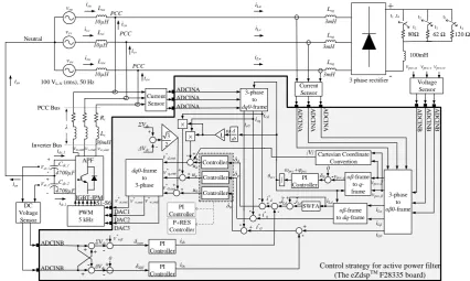
The harmonic elimination system using the APF is shown in Fig. 1. From Fig. 1, there are four parts. In the first part, the considered power system is the balanced three-phase system. The second part is the APF topology [12]. In this paper, the three-leg split-capacitor topology [13, 14] is used to inject the compensating currents for harmonic elimination. The third part is the harmonic identification by using DQF method [15]. The last part is the control strategy. The aim of this paper is the performance improvement of the compensating current controller. Because it is significant to achieve the good performance for harmonic elimination. This paper presents the performance comparison of the compensating current controllers. The proportional plus resonant (P+RES) controller [16, 17] is considered to compare the performance with the proportional integral (PI) controller [18]. These controllers provide a small tracking error in steady state. However, when the non-linear load is changed, the P+RES controller can be adapted to control the compensating currents following on the significant harmonic orders in the system. Therefore, the P+RES controller can provide better results compared with PI controller.
isu isv isw iLu iLv iLw icw icv icu i* 0 i* d i* q PCC PCC PCC Lsu Lsv Lsw Leq Leq Leq Neutral
100 VL-N (rms), 50 Hz 3 phase rectifier
vpcc,uvpcc,vvpcc,w
APF isn icn idc,1 idv i0v vsu vsv vsw iLα iLβ + -vpcc,α
vpcc,β 3-phase
to
αβ0-frame
αβ-frame to dq-frame
iL0 Lc Rc 3-phase to dq0-frame v* ref 0 Controller PI Controller PI Controller PWM 5 kHz dq0-frame to 3-phase ΣVdc ΔVdc -+ + θpcc L × × ω |V| dt d ΣVdc ΔVdc -+ 2 3 + + + + - + + δ d δq δ0 icd icq ic0 -+ +
+ iLd iLd
~ Ld i uq u0 ud v* 0,out v* q,out v* d,out v* u,out δsum δdiff v* v,outv*w,out
Control strategy for active power filter (The eZdspTM
F28335 board)
αβ-frame
to q -frame vpcc,q Cartesian Coordinate Convertion PI Controller 0 -δθ
ωpcc+φpcc
idc,2
PCC Bus
Inverter Bus v
u,outvv,outvw,out
λ P+RES Controller PI Controller Controller Controller DC Voltage Sensor ADCINB ADCINB Voltage Sensor Current Sensor ADCINA ADCINA ADCINA Current Sensor A D C IN A A D C IN A A D C IN A DAC1 DAC2 DAC3 IGBT-IPM A D C IN B A D C IN B A D C IN B + -t1 ,t4
100mH
80 62 120
t2 t2 t3 t3 t4 S1-S6
Fig. 1. Considered power system and control strategy.
[image:2.595.82.509.354.609.2]The paper is structured as follows. The design of the PI and P+RES controllers are described in Section 2. The experimental setup is expressed in Section 3. In Section 4, the experimental results and discussion are also shown. Finally, Section 5 concludes the advantage of the P+RES controller.
2.
The Compensating Current Control
2.1. The Design of The PI Controller
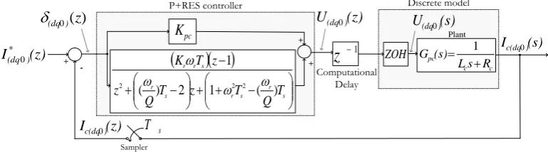
The discrete design approach [28] is used to design the PI controller. This approach is suitable for the digital control. The block diagram to design the PI controllers on dq0-frame are illustrated in Fig. 2.
PI controller pc K + + Plant + -(z) U(dq0)
ZOH
) ( 0) z (dq c c pc R s L (s) G 1 1
z
Computational Delay s T Sampler (z) Ic(dq0)(s) Ic(dq0)
Discrete model (s) U(dq0)
(z) I(dq* 0)
1 z
T
Kic s
Fig. 2. The block diagram to design the PI controllers on dq0-frame.
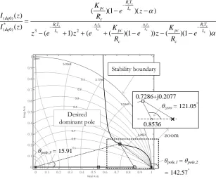
[image:3.595.109.491.220.330.2]From the block diagram in Fig. 2, the closed-loop transfer function can be derived in Eq. (1). From Eq. (1), the parameters of and Kpc are calculated by using the root-locus technique on Z-plane as shown in Fig. 3. ) 1 )( ( )) 1 )( ( ( ) 1 ( ) )( 1 )( ( ) ( ) ( 2 3 * ) 0 ( ) 0 ( c s c c L s T c R c L s T c R c s c c s c L T R c pc c pc L T R L T R c pc dq dq e R K z e R K e z e z z e R K z I z I (1)
0 0.1 0.2 0.3 0.4 0.5 0.6 0.7 0.8 0.9 1 0 0.1 0.2 0.3 0.4 0.5 0.6 0.7 0.8 0.9 1 1.26e4 2.51e4 3.77e4 5.03e4 6.28e4 0.1 0.2 0.3 0.4 0.5 0.6 0.7 0.8 0.9
Root Locus Editor for Open Loop 1(OL1)
Real Axis Im a g A x is Stability boundary Desired dominant pole
θpole,3 = 15.91
°
zoom
θpole,1 = θpole,2
= 142.57°
θzero = 121.05°
0.8536 0.7286+j0.2077
Fig. 3. The root – locus of the compensating current control.
[image:3.595.141.449.422.677.2]2077 . 0 7286 . 0 ) 1 ( 2 j e
z Tsnjn (2)
For =0.8536 and Kp c =262.66, the appropriate PI controller parameters are Kp c =262.66, Kic
=1.54×10⁶. The details of the PI controller design can be found in the previous publications [18].
2.2. The Design of The Proportional plus Resonant Controller
The P+RES controller is developed from the PI controller [16]. The block diagram considered the discrete design approach is depicted in Fig. 4. From Fig. 4, the root locus can be explained by using the closed-loop transfer function in Eq. (2). The placement of poles and zero on Z-plane are shown in Fig. 5. The poles of the closed-loop transfer function in Eq. (2) must be located in the stability boundary (unit circle on Z -plane). P+RES controller pc K + + Plant + -(z) U(dq0)
ZOH
) ( 0) z (dq c c pc R s L (s) G 1 1
z
Computational Delay s T Sampler (z) Ic(dq0)(s) Ic(dq0)
Discrete model (s) U(dq0)
s r s r s r s r r T Q T z T Q z z T K ) ( 1 2 ) ( 1 2 22
(z) I*
) (dq0
Fig. 4. The block diagram to design the P+RES controllers on dq0-frame.
A T L C T L K z C A T L B T L K z B C T L K z B z K A C z K A B z T L K z I z I s c s c pc s c s c pc s c pc pc pc s c pc dq dq 2 3 4 2 * ) 0 ( ) 0 ( 1 ) ( ) ( (2)where AKrrTs
,
B(r/Q)Ts2,
C 1 rTs ( r/Q)Ts2
2
0.96 0.965 0.97 0.975 0.98 0.985 0.99 0.995 1 1.005
0.035 0.04 0.045 0.05 0.055 0.06 0.065 0.07 Real Axis Im a g A x
is pole of resonant
term
Q increasing
Q
decreasing
stability boundary
zero of resonant term
Kr inc
reasing
Kpc dec
reasing
Kr dec
reasing
Kpc inc
reasing
ζ = 0.7
ζ = 0.8 ζ = 0.5
ζ = 0.6
ζ = 0.4 ζ = 0.3
ζ = 0.2
Q increas
ing
Q decreas
[image:4.595.105.490.258.365.2]Fig. 5. The placement of zero and pole on Z-plane.
The parameters of the P+RES controller consist of the proportional gain (Kpc), the gain of resonant term (Kr), the resonant frequency (r) and the quality factor (Q). The resonant frequency (r) in the
P+RES controllers can be adjusted depending on the significant harmonic frequency on dq0-frame. The spectra of the reference currents on dq0-frame ( *
d i ,i*q,
* 0
i ) are shown in Fig. 6. Therefore, therd , rq and
0 r
are set to2300, 2300and 0 rad/s, respectively.
Decreasing load currents
Considered load currents
Increasing load currents
frequency (Hz)
0 100 200 300 400 500 600 700 800 900 1000
0 1 2
0 100 200 300 400 500 600 700 800 900 1000
0 1 2
0 100 200 300 400 500 600 700 800 900 1000
0 1 2
Significant order
Significant order
* d i
*
q
i
* 0 i
Fig. 6. The spectra of the reference currents on dq0-frame.
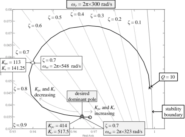
For example on dq-axis (r=2π×300 rad/s), theKpcandKrare designed depending on specific values
(ωni =2π×300 rad/s, ζ =0.7). The root locus technique on Z-plane is used to obtain the desired dominant pole. (Kp c=414,Kr =517.5) as shown in Fig. 7.
0.93 0.94 0.95 0.96 0.97 0.98 0.99 1
0.03 0.035 0.04 0.045 0.05 0.055 0.06 0.065 0.07 0.075 0.08
Real Axis
Im
a
g
A
x
is
Kpc = 113 Kr = 141.25
Kpc = 414 Kr = 517.5
stability boundary
ωr = 2π×300 rad/s
desired dominant pole
Kpc and Kr
decreasing
Kpc and Kr
increasing ζ = 0.6
ζ = 0.8
ζ = 0.4
ζ = 0.5 ζ = 0.3 ζ = 0.2
ζ = 0.1
ζ = 0.7
ζ = 0.9
ζ = 0.7
ωni = 2π×548 rad/s
ζ = 0.7
ωni = 2π×323 rad/s
Q = 10
Fig. 7. The criteria for designingKpcandKr.
The characteristic of quality factor (Q) is shown in Fig. 7. The Q can be calculated by Eq. (3). From
[image:5.595.155.452.190.353.2] [image:5.595.147.458.452.683.2]should be selected in the boundary as shown in Eq. (4). The boundary of Q in this case is 1.5<Q<150.
Therefore, The Q is defined to 10 (fr=300 Hz, fH= 315 Hz, fL=285 Hz). Moreover, according to Fig. 7,
the pole of resonant term at Q=10is located in the stable region.
10-3 10-2 10-1
-160 -150 -140 -130 -120 -110 -100 -90 -80 -70 -60
M
a
g
n
itu
d
e
(
d
B
)
Bode Diagram
Frequency (rad/s)
Magnitude (abs)
|Kr|
0.707|Kr|
Frequency (rad/s)
fL fr fH
Δf1
Δf2
Δf1 = fr – fL
Δf2 = fH - fr
Fig. 8. The characteristic of quality factor (Q).
L H
r
f f
f Q
(3)
max
min Q Q
Q (4)
where
100 100
1 2
min
r r
r r
f f
f f
f f
Q and
1
1
1 2
max
r r
r r
f f
f f
f f Q
3.
Experimental Setup
The experimental setup for the harmonic elimination system using an APF consists of two main parts. The first part is the experimental rig as shown in Fig. 9. It can be seen in Fig. 9 that the experimental rig can be decomposed into four sections. The first section is the considered power system. The three-phase voltage source connected with the three-phase rectifiers is shown in number 1 to 5. The second section is the voltage/current sensors and signal conditioning circuits as shown in number 6. The PCC voltages (vpcc,(uvw))
are measured by using the transformers (220Vac /15Vac). The DC bus voltages (Vd c,1,Vd c,2) are measured by
using the voltage transducers (LEM LV25-P). The load currents (iL(u vw)) and compensating currents (ic(u vw))
are measured by using the current transducers (LEM HX10-P). The range of all measured signals (vpcc,(uvw),
) 2 , 1 ( , d c
V ,iL(u vw),ic(u vw)) for the DSP board are adjusted by signal conditioning circuits. The third section is the
control platform as shown in number 7 and 8. This section consists of three processes to generate the pulse signals (S1-S6). First, the host computer provides the user interface to the DSP board. The eZdspTM
F28335 board calculates the reference voltages of APF ( * ), (uvwout
v ) from the proposed control strategy. Second, the D/A converters (DAC712P) are used to transform the *
), (uvwout
v from the digital signals to the analog signals. Third, the analog signals of *
), (uvwout
v (reference signals) are sent to compare with the triangular carriers in PWM modulator. The pulse signals (S1-S6) from the PWM technique are sent to drive the insulated-gate bipolar transistors (IGBTs) of the APF. The fourth section is the APF topology as shown in number 9 to 11. The capacitors (Cd c,1=Cd c,2=4700 μF) are connected with IGBT-Intelligent Power Module
(IPM) (6MBP50RA-120) on the DC side. The APF inductances (Lc(u vw)=18 mH) are connected with
IGBT-IPM on the AC side. The APF injects theic(u vw)into the considered power system at the PCC points (number
1. Three-phase voltage source 2. Source inductance
3. Point of common coupling 4. Line inductance
5. Three-phase rectifier 6. Voltage/Current sensors and Signal conditioning circuits 7. eZdspTMF28335, D/A converter and PWM modulator
8. Host Computer
9. IGBT-IPM and Gate drive circuit 10. DC Bus capacitors
11. APF inductance 12. Power quality analyzer 12
1
2
3
4
5
6
7
8
9
10 11
Fig. 9. The overall of experimental rig.
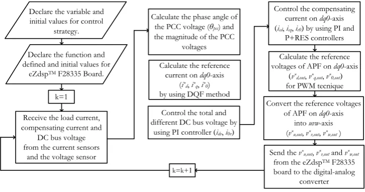
The second part is the software for the control of the APF. The code composer studio (CCS v3.3) is used to program on eZdsp F28335 board. The overall flowchart to control the APF can be described in Fig. 10. The phase locked loop algorithm, the DQF harmonic detection, the DC bus voltage control (PI), the compensating current control (PI, P+RES) and control strategy on dq0-axis are written in C programming languages by using the CCS v3.3.
Receive the load current, compensating currentand
DC bus voltage from the current sensors
and the voltage sensor k=1
Calculate the reference current on dq0-axis
(i*d, i*q, i*0) by using DQF method
Control the total and different DC bus voltage by
using PI controller (idv, i0v)
Control the compensating current on dq0-axis
(icd, icq, ic0) by using PI and P+RES controllers
Calculate the reference voltages of APF on dq0-axis
(v*d,out, v*q,out, v*0,out)
for PWM tecnique
Convert the reference voltages of APF on dq0-axis
into uvw-axis (v*u,out, v*v,out, v*w,out)
k=k+1
Declare the function and defined and initial values for
eZdspTM F28335 Board. Declare the variable and initial values for control
strategy.
Calculate the phase angle of the PCC voltage (θpcc) and themagnitude of the PCC
voltages
Send the v*u,out, v*v,out and v*w,out from the eZdspTM F28335 board to the digital-analog
[image:7.595.70.515.90.278.2]converter
Fig. 10. Flowchart of the harmonic identification and control strategy.
4.
Experimental Results and Discussion
The harmonic identification and control strategy in Fig. 1 are supported by the hardware implementation. The APF parameters are designed following on the previous researches [29, 30]. The harmonic elimination results for the balanced three-phase system are depicted in Fig. 11–12.
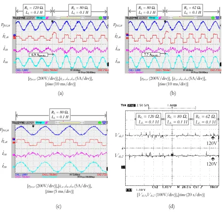
The performance of the proposed controller for harmonic elimination using the APF are tested with three load conditions. The first load condition is the amplitude of load currents at 2 A(peak) (RL=120 Ω, LL=0.1H). The second load condition is the amplitude of load currents at 3 A(peak) (RL=80 Ω, LL=0.1H).
The third load condition is the amplitude of load currents at 4 A(peak) (RL=62 Ω, LL=0.1H).
[image:7.595.117.480.387.578.2]harmonic distortion (%THDav) of this current is equal to 29.3 %, as shown in Fig. 13 (a). After compensation, the APF injects the compensating current (icu,icv,icw) into the considered power system at a
PCC point. The source currents after compensation ( isu ,isv ,isw ) are nearly sinusoidal waveform.
The %THDav is equal to 10.66 %, as shown in Fig. 13 (b). According to Fig. 11(a)-(b), for the dynamic load testing, when the non-linear load resistor (RL) is changed from 120 Ω to 80 Ω and 80 Ω to 62 Ω, the waveforms of is(u vw)after compensation are oscillating sinusoidal waveform. The peak amplitude of isu is
equal to 5.80 A(peak) (4.10 A(rms)) and 7.35 A(peak) (5.20 A(rms)), respectively. In the steady state condition, the
su
i is constant at 4.20 A(peak) (2.97 A(rms)) and 4.95 A(peak) (3.5 A(rms)), respectively. From Fig. 11(d), the total
DC bus voltage loop control can regulate the total DC bus voltage (
Vdc) following on the total DC busreference (
*dc
V ) even though the loads are varied. It can be seen from Fig. 11(d) that the Vd c,1and Vdc,2
are equal to 120 V. Therefore, the
Vdcis constant at 240 V. The results in Fig. 11(d) confirm that the PIcontrollers of the DC bus voltage control provide good performance.
v
pcc,ui
Lui
cui
suv
pcc,ui
Lui
cui
suv
pcc,ui
Lui
cui
su[vpcc,u(200V/div)],[iLu ,icu ,isu (5A/div)],
[time(10 ms/div)]
[vpcc,u(200V/div)], [iLu ,icu ,isu (5A/div)],
[time(10 ms/div)]
[vpcc,u(200V/div)], [iLu ,icu ,isu (5A/div)],
[time(5 ms/div)]
[Vdc,1,Vdc,2(100V/div)],[time(20 s/div)]
V
dc,1V
dc,2RL = 80 ,
LL = 0.1 H
RL = 120 ,
LL = 0.1 H
RL = 62 ,
LL = 0.1 H
120V
120V
RL = 80 , LL = 0.1 H RL = 120 ,
LL = 0.1 H
RL = 62 , LL = 0.1 H RL = 80 ,
LL = 0.1 H
RL = 80 ,
LL = 0.1 H
(a)
(b)
(c)
(d)
[image:8.595.74.530.269.705.2]5.8 A(peak) 7.30 A(peak)
Fig. 11. The testing results of harmonic elimination with PI controller. (a) The peak amplitude of load current changing from 2 A(peak) to 3 A(peak), (b) The peak amplitude of load current changing from 3 A(peak)
to 4 A(peak), (c) The amplitude of load currents at 3 A(peak), (d) The performance of the DC bus voltage
v
pcc,ui
Lui
cui
suv
pcc,ui
Lui
cui
suv
pcc,ui
Lui
cui
su120V
120V
[Vdc,1,Vdc,2(100V/div)],[time(20 s/div)]
Vdc,1
Vdc,2
RL = 80 ,
LL = 0.1 H
RL = 120 ,
LL = 0.1 H
RL = 62 ,
LL = 0.1 H
[vpcc,u(200V/div)],[iLu ,icu ,isu (5A/div)],
[time(10 ms/div)]
[vpcc,u(200V/div)], [iLu ,icu ,isu (5A/div)],
[time(10 ms/div)]
[vpcc,u(200V/div)],[iLu ,icu ,isu (5A/div)],
[time(5 ms/div)] RL = 80 ,
LL = 0.1 H
RL = 120 ,
LL = 0.1 H
RL = 62 ,
LL = 0.1 H
RL = 80 ,
LL = 0.1 H
RL = 80 ,
LL = 0.1 H
(a) (b)
(c) (d)
[image:9.595.75.532.84.514.2]6.9 A(peak) 7.7 A(peak)
Fig. 12. The testing results of harmonic elimination with P+RES controller. (a) The peak amplitude of load current changing from 2 A(peak) to 3 A(peak), (b) The peak amplitude of load current changing from 3 A(peak)
to 4 A(peak), (c) The amplitude of load currents at 3 A(peak), (d) The performance of the DC bus voltage
control.
The results of the harmonic elimination using a P+RES controller are shown in Fig. 12 (a)-(c). From the results in Fig. 12 (a)-(c), this controller provides the good performance for harmonic elimination. The %THDav after compensation is equal to 9.28 %, as shown in Fig. 13 (c). Therefore, the performance of the harmonic elimination with the P+RES controller is better than that from the PI controller. From the dynamic load testing, fig. 12 (a) and (b) show the waveform of is(u vw) to a step change of the RL from 120 Ω
to 80 Ω and 80 Ω to 62 Ω, respectively. It can be seen that the waveforms of is(u vw) are oscillating sinusoidal
waveform. The peak amplitude of isu is equal to 6.90 A(peak) (4.88 A(rms)) and 7.70 A(peak) (5.44 A(rms)),
respectively. In the steady state condition, the isu is still constant at 4.20 A(peak) (2.97 A(rms)) and 4.95 A(peak)
(3.5 A(rms)), respectively. As a result, the transient response of the isu from P+RES controller are nearlythe
same as the transient response of the isu from PI controller. However, the focus of this paper is to achieve
the performance of the harmonic elimination (%THD). From the results in Fig. 12 (d), the Vd c,1and Vd c,2
5.93%
4.10% 4.27%
3.50% 23.04%
10.64%
(a)
(b)
(c)
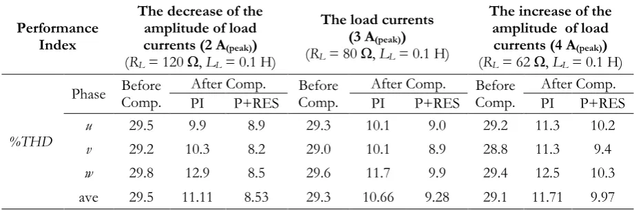
Fig. 13. The spectrum of source currents. (a) Before compensation, (b) After compensation (PI controller), (c) After compensation (P+RES controller).
Table 1. The performance of the source currents before and after compensations.
Performance Index
The decrease of the amplitude of load currents (2 A(peak))
(RL = 120 Ω, LL = 0.1 H)
The load currents
(3 A(peak))
(RL = 80 Ω, LL = 0.1 H)
The increase of the amplitude of load currents (4 A(peak))
(RL = 62 Ω, LL = 0.1 H)
%THD
Phase Before Comp. PI After Comp. P+RES Comp. Before After Comp. PI P+RES Comp. Before PI After Comp. P+RES
u 29.5 9.9 8.9 29.3 10.1 9.0 29.2 11.3 10.2
v 29.2 10.3 8.2 29.0 10.1 8.9 28.8 11.3 9.4
w 29.8 12.9 8.5 29.6 11.7 9.9 29.4 12.5 10.3 ave 29.5 11.11 8.53 29.3 10.66 9.28 29.1 11.71 9.97
In addition, the APF topology as shown in Fig. 1 can compensate the harmonic current in the unbalanced three-phase system. But the testing for the harmonic elimination in this work is only considered in the balanced three-phase system. However, the authors will test the unbalanced three-phase system in the future work.
5.
Conclusion
The PI and the proportional plus resonant (P+RES) controllers are designed by discrete design approach. The design of PI and P+RES controllers are fully presented in this paper. The harmonic elimination system with the three-leg split-capacitor APF and the overall control strategy on dq0-axis have been implemented. In the paper, the performance comparison of the compensating current control using the PI and the P+RES controllers is tested with dynamic load changing. The experimental results confirm that the proposed control strategy based on digital control is very useful to mitigate the harmonics in the system. The results show that the P+RES controller can provide the good performance of the harmonic elimination compared with the PI controller in term of %THD.
Acknowledgements
[image:10.595.76.523.82.214.2] [image:10.595.67.534.293.446.2]References
[1] IEEE Recommended Practices and Requirement for Harmonic Control in Electrical Power System, IEEE Std. 519-2014, 2014.
[2] A. D. Graham and E. T. Schonholder, “Line harmonics of converters with DC motor loads,” IEEE Transactions on Industry Applications, vol. IA-19, no. 1, pp. 84-93, Jan. 1983.
[3] G. C. Jain, “The effect of voltage waveshape on the performance of a three-phase induction motor,”
IEEE Transactions on Power Apparatus and Systems, vol. 83, no. 6, pp. 561-566, Jun. 1964.
[4] IEEE Standard General Requirements for Liquid-Immersed Distribution, Power, and Regulating Transformers, IEEE Std. C57.12.00-1987, 1988.
[5] IEEE Recommended Practice for Establishing Transformer Capability When Supplying Non-sinusoidal Load Currents, IEEE Std. C57.110-1986, 1986.
[6] IEEE Standard for Shunt Power Capacitors, IEEE Std. 18-2002, 2002.
[7] W. C. Downing, “Watthour meter accuracy on SCR controlled resistance loads,” IEEE Transactions on Power Apparatus and Systems, vol. PAS-93, no. 4, pp. 1083-1089, Jul. 1974.
[8] Power System Relaying Committee, “The impact of sine-wave distortions on protective relays,” IEEE Transactions on Industry Applications, vol. IA-20, no. 2, pp. 335-343, Mar. 1984.
[9] L. Gyugyi and E. C. Strycula, “Active AC power filters,” in Proceedings of IEEE Industry Applications Annual Meeting, San Diego, CA, September 11-13, 1989.
[10] F. Z. Peng, H. Akagi, and A. Nabae, “A new approach to compensation in power systems,” in
Conference Record of the 1988 IEEE Industry Applications Society Annual Meeting, Pittsburgh, PA, USA, October 2-7, 1988.
[11] C. A. Quinn and N. Mohan, “Active filtering of harmonic currents in three-phase, four-wire systems with three-phase and single-phase non-linear loads,” in IEEE-APEC’92 Appl. Power Electronics Conference, 1992, pp. 829-836.
[12] V. Khadkikar, A. Chandra, and B. Singh, “Digital signal processor implementation and performance evaluation of split capacitor,” IET Power Electronics, vol. 4, no. 4, pp. 463-470, 2011.
[13] M. Aredes, J. Hafner, and K. Heumann, “Three-phase four-wire shunt active filter control strategies,”
IEEE Transactions on Power Electronics, vol. 12, no. 2, pp. 311-318, 1997.
[14] M. Aredes, J. Hafner, and K. Heumann, “A three-phase four-wire shunt active filter using six IGBT’s,” in Proc. EPE’95-European Conference Power Electronics Applications, Pittsburgh, Sevilla, Spain, Sept. 1995, vol. 1.
[15] S. Sujitjorn, K.-L. Areerak, and T. Kulworawanichpong, “The DQ axis with fourier (DQF) method for harmonic identification,” IEEE Transactions on Power Delivery, vol. 22, no. 1, pp. 737-739, Dec. 2006. [16] Y. Sato, T. Ishizuka, K. Nezu, and T. Kataoka, “A new control strategy for voltage-type PWM
rectifiers to realize zero steady-state control error in input current,” IEEE Transactions on Industry Applications, vol. 34, no. 3, pp. 480-486, May/June 1998.
[17] W. Lenwari, M. Sumner, and P. Zanchetta, “The use of genetic algorithms for the design of resonant compensator for active filters,” IEEE Transaction on Industrial Electronics, vol. 56, no. 8, pp. 2852-2861, Apr. 2009.
[18] P. Santiprapan, K.-L. Areerak, and K.-N. Areerak, “Dynamic model and controller design for active power filter in three-phase four-wire system,” International Journal of Control and Automation, vol. 7, no. 9, pp. 27-44, Sep. 2014.
[19] C. Qiao, K. M. Smedley, and F. Maddaleno, “A single-phase active power filter with one-cycle control under unipolar operation,” IEEE Transactions on Circuits and Systems I: Regular Papers, vol. 51, no. 8, pp. 1623-1630, Aug. 2004.
[20] K. M. Tsang and W. L. Chan, “Design of single-phase active power filter using analogue cascade controller,” IEE Proceedings - Electric Power Applications, vol. 153, no. 5, pp. 735-741, Oct. 2006.
[21] J. Miret, L. G. de Vicuna, M. Castilla, J. Matas, and J. M. Guerrero, “Design of an analog quasi-steady-state nonlinear current-mode controller for single-phase active power filter,” IEEE Transactions on Industrial Electronics, vol. 56, no. 12, pp. 4872-4881, Dec. 2009.
[23] S. Rahmani, N. Mendalek, and K. Al-Haddad, “Experimental design of a nonlinear control technique for three-phase shunt active power filter,” IEEE Transactions on Industrial Electronics, vol. 57, no. 10, pp. 3364-3375, Oct. 2010.
[24] M. Popescu, A. Bitoleanu and V. Suru, “A DSP-based implementation of the p-q theory in active power filtering under nonideal voltage conditions,” IEEE Transactions on Industrial Informatics, vol. 9, no. 2, pp. 880-889, May 2013.
[25] T. Narongrit, K.-L. Areerak, and K.-N. Areerak, “Adaptive fuzzy control for shunt active power filters,” Electric Power Components and Systems, vol. 44, no. 6, pp. 646-657, Mar. 2016.
[26] Z. Shu, M. Liu, L. Zhao, S. Song, Q. Zhou, and X. He, “Predictive harmonic control and its optimal digital implementation for MMC-based active power filter,” IEEE Transactions on Industrial Electronics, vol. 63, no. 8, pp. 5244-5254, Aug. 2016.
[27] A. S. Lock, E. R. C. da Silva, M. E. Elbuluk, and D. A. Fernandes, “An APF-OCC strategy for common-mode current rejection,” IEEE Transactions on Industry Applications, vol. 52, no. 6, pp. 4935-4945, Nov.-Dec. 2016.
[28] G. F. Franklin, J. D. Powell, and A. Emami-Naeini, Feedback Control of Dynamic Systems, 4th ed. Upper Saddle River, NJ, USA: Prentice-Hall, 2002.
[29] T. Thomas, K. Haddad, G. Joos, and A. Jaafari, “Design and performance of active power filters,”
IEEE Industry Application Magazine, vol. 4, no. 5, pp. 38-46, Sep.-Oct. 1998.