Inferring Drosophila gap gene regulatory network: pattern analysis of simulated gene expression profiles and stability analysis

(1)

Open Access

Short Report

Inferring Drosophila gap gene regulatory network: pattern analysis

of simulated gene expression profiles and stability analysis

Yves Fomekong-Nanfack

†

_{, Marten Postma}

†

_{and Jaap A Kaandorp*}

Address: Section Computational Science, Faculty of Science University of Amsterdam. Science Park 107, 1078 XJ, Amsterdam, The Netherlands

Email: Yves Fomekong-Nanfack - [email protected]; Marten Postma - [email protected]; Jaap A Kaandorp* - [email protected] * Corresponding author †Equal contributors

Abstract

Background: Inference of gene regulatory networks (GRNs) requires accurate data, a method to simulate the expression patterns and an efficient optimization algorithm to estimate the unknown parameters. Using this approach it is possible to obtain alternative circuits without making any a priori assumptions about the interactions, which all simulate the observed patterns. It is important to analyze the properties of the circuits.

Findings: We have analyzed the simulated gene expression patterns of previously obtained circuits that describe gap gene dynamics during early Drosophila melanogaster embryogenesis. Using hierarchical clustering we show that amplitude variation and defects observed in the simulated gene expression patterns are linked to similar circuits, which can be grouped. Furthermore, analysis of the long-term dynamics revealed four main dynamical attractors comprising stable patterns and oscillatory patterns. In addition, we also performed a correlation analysis on the parameters showing an intricate correlation pattern.

Conclusions: The analysis demonstrates that the obtained gap gene circuits are not unique showing variable long-term dynamics and highly correlating scattered parameters. Furthermore, although the model can simulate the pattern up to gastrulation and confirms several of the known regulatory interactions, it does not reproduce the transient expression of all gap genes as observed experimentally. We suggest that the shortcomings of the model may be caused by overfitting, incomplete model description and/or missing data.

Introduction

A biological system that has been extensively studied is the segmentation mechanism of early development in Drosophila melanogaster (see [1] for review). At early stage, a cascade of maternal and zygotic genes is activated in the syncytial embryo that subdivides the ectoderm into smaller domains. First, maternal morphogenes such as bicoid (bcd), caudal (cad) and hunchback (hb) activate zygotic gap genes such as hb, giant (gt), Krüppel (Kr), knirps (kni), or tailles (tll), which in turn will activate the pair rule

genes. The pair rule genes will regulate segment polarity genes and Hox genes, which both control the differentia-tion of each segment of the future embryo [1].

The gap gene circuit has been extensively investigated using mathematical models [2,3]. In all cases, the goal was to derive the regulatory interactions that control gene expression. The gene circuit approach [4] combined with a parameter optimization method allowed to infer gene regulatory interactions directly from experimental

spatio-Published: 16 December 2009

BMC Research Notes 2009, 2:256 doi:10.1186/1756-0500-2-256

Received: 10 June 2009 Accepted: 16 December 2009

This article is available from: http://www.biomedcentral.com/1756-0500/2/256

(2)

temporal gene expression data [5,6]. In all cases the opti-mization involved miniopti-mization of the difference between observed data and simulated data. Previous stud-ies [4,7,8] have analyzed the obtained gene circuits essen-tially by visual inspection of the simulated patterns, mainly because of an insufficient number of circuits. Fomekong et al. [8] proposed a faster optimization method that yielded a higher number of circuits, allowing for a more detailed analysis. Finding a set of parameters that reproduces the observed data does not necessary imply that the network structure has been identified cor-rectly, or that the underlying pattern formation mecha-nism of the system has been revealed [9,10]. For some systems, the network structure itself inherently leads to robust pattern formation and is weakly depended on the specific parameter values [11,12]. Inference may lead to a unique network, however for many cases many circuits with different topologies and scattered parameter values are found. It is necessary to further analyze these circuits

and discriminate between realistic and non-realistic cir-cuits based on other criteria [13,14].

We have analyzed the simulated patterns and parameters of the circuits that were obtained previously using descrip-tive statistics and stability analysis [8,15]. The incomplete-ness of the available experimental data, the complexity and the non-linearity of the model and the large number of unknown parameters potentially leading to over-fitting makes the reverse engineering problem challenging. It might lead to circuits with different regulatory interac-tions or variability in the simulated patterns and dynami-cal behavior.

Findings

Simulated profiles

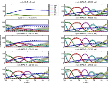
Although all circuits show relatively good fits with respect to the data (see Figure 1), small features, like bumps, dips and other variations in the expression profiles at

[image:2.612.114.494.98.401.2]

gastrula-Expression profiles of the 101 gap gene circuits at different time points

Figure 1

Expression profiles of the 101 gap gene circuits at different time points. Individual gene profiles are shown in light gray and the average profile of that gene at a specific time point is plotted using a colored solid lines. The x-axis corresponds to 35-92% of the A-P position and the y-axis describes the expression level influorescence units. Each panel corresponds to one of the 10 time points (12, 13 and 14A1-14A8) for which data are available. The experimentally measured expression profiles are plotted using colored dashed lines.

0 100 200

cycle 12 (T = 0 min)

cad hb Kr gt kni tll

0 100 200

cycle 13 (T = 10.55 min)

0 100 200

cycle 14A1 (T = 24.225 min)

expression level

0 100 200

cycle 14A2 (T = 30.475 min)

35 44 54 64 74 84 92 0

100 200

cycle 14A3 (T = 36.725 min)

position

0 100 200

cycle 14A4 (T = 42.975 min)

0 100 200

cycle 14A5 (T = 49.225 min)

0 100 200

cycle 14A6 (T = 55.475 min)

0 100 200

cycle 14A7 (T = 61.725 min)

35 44 54 64 74 84 92 0

100 200

cycle 14A8 (T = 67.975 min)

(3)

Hierarchical clustering of simulated profiles at T = 68.1 min

200 tll

(4)

[image:4.612.141.467.92.427.2]

Dendrograms obtained from hierarchical clustering of the simulated profiles at T = 68.1 min

Figure 3

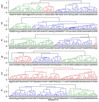
Dendrograms obtained from hierarchical clustering of the simulated profiles at T = 68.1 min. Each Individual tree diagram corresponds to the distribution of all the profiles obtained from the different circuits for a single gene. In each tree, the circuits belonging to the same cluster are grouped.

0 0.5 1

9 64 28 79 42 83 31 95 6 40 24 94 87 32 3 78 96 99 52 81 70 98 100 68 12 53 97 25 47 57 77 19 43 27 37 45 54 76 8 14 71 16 74 93 50 44 10 75 69 84 29 49 1 65 66 88 2 13 30 82 33 39 7 38 21 62 72 4 86 22 92 51 90 101 11 20 36 80 26 5 17 18 67 23 41 89 15 35 34 48 46 58 60 55 63 56 59 61 73 85 91

cad

0 0.5 1

61 91 85 46 59 86 48 6 35 73 76 100 5 23 18 89 56 63 67 54 41 17 34 55 58 60 1 94 27 45 44 2 19 88 57 16 77 43 70 40 50 15 32 64 3 79 20 26 78 28 24 101 51 31 83 52 95 96 99 98 80 53 81 4 9 72 84 8 13 14 39 11 12 36 22 93 42 7 38 25 47 69 82 71 75 90 92 74 30 37 49 33 68 87 97 10 21 65 62 66 29

hb

0 0.5 1

96 99 52 31 83 85 5 46 48 12 80 67 40 55 20 42 36 53 90 22 34 9 11 101 10 29 82 78 97 49 51 95 7 74 14 26 25 47 38 81 8 69 71 75 98 72 13 92 33 68 84 1 76 44 16 57 73 88 21 2 56 86 70 4 24 32 94 50 3 28 79 30 65 39 66 15 23 17 62 77 93 18 89 6 35 41 58 59 54 64 63 87 91 60 61 19 27 45 43 100 37

Kr

0 0.5 1

19 45 27 43 37 5 40 52 53 95 96 99 97 11 51 90 98 100 9 12 42 20 36 31 79 101 6 35 63 46 48 55 60 41 15 32 94 54 67 64 76 58 73 93 80 83 87 17 34 85 91 59 61 89 18 56 23 29 49 86 1 16 2 57 62 4 30 39 7 22 84 65 69 71 72 75 44 66 88 24 70 50 77 33 3 14 26 28 78 10 21 8 13 38 68 74 82 92 25 47 81

gt

0 0.5 1

96 99 100 54 85 93 23 77 58 63 64 6 83 98 73 76 50 56 57 59 87 53 97 5 67 60 91 9 80 46 48 18 32 89 94 15 55 17 61 41 35 40 52 81 1 31 16 86 24 88 2 65 66 37 38 25 47 26 101 3 11 14 8 71 72 36 74 84 4 69 75 30 43 39 82 13 92 68 90 19 27 45 29 12 42 34 28 78 79 10 44 49 21 51 95 7 33 20 22 62 70

kni

0 0.5 1

19 69 75 43 74 28 37 45 70 100 14 26 53 81 25 101 68 84 78 82 3 98 11 79 52 95 51 12 87 96 99 1 88 2 30 31 39 66 44 65 16 57 90 21 62 13 27 92 77 4 7 8 36 22 71 72 20 47 42 80 83 24 38 33 97 50 94 5 10 17 9 64 6 76 41 54 15 32 29 93 49 73 56 59 18 23 89 58 63 67 34 55 60 85 86 91 46 35 61 40 48

tll

solution nr

Table 1: Parameter differences between circuits of group 1 and circuits of group 2-3.

parameter differences between circuits of group 1 and group 2-3

θ m1 m2 dm p - value

tll →cad -0.0171377 -0.02491 -0.00777229 1.04553e - 010

hb →hb 0.0217064 0.015097 -0.00660943 1.34364e - 011

gt →hb 0.0122061 -0.00414659 -0.0163527 0

kni →hb -0.128935 -0.0747608 0.0541739 5.28773e - 009

Kr →Kr 0.0161343 0.0227917 0.00665739 4.79087e - 007

gt →Kr -0.0528814 -0.027446 0.0254355 2.71076e - 010

hb →gt -0.003434 0.00397726 0.00741126 8.47311e - 011

gt →gt 0.0132754 0.0164244 0.00314898 2.4076e - 006

tll →gt -0.0155584 -0.0438868 -0.0283284 1.11022e - 015

gt →tll -0.0252096 -0.00316618 0.0220435 3.74904e - 007

m →Kr 0.0525071 0.0306038 -0.0219033 6.33614e - 007

m →gt 0.0703723 0.0261228 -0.0442495 8.70947e - 009

T-test comparison of circuit parameters belonging to a group with a normal pattern without any defection (group 1) and a solution for which hb has a dip and tll a bump (group 2 and 3).

[image:4.612.55.559.518.679.2]

(5)

tion time are observed (see Additional file 1). These fea-tures are not observed in the data, and may represent circuits that are not biologically realistic. We performed a hierarchical cluster analysis on the profiles to identify groups that share deviant features. By statistical compari-son of the parameters among the different groups using a T-test we find parameters that may explain the observed features.

Figure 2 shows the clustered simulated profiles where we observe four main pattern groups described as follows: group 1: no defection. group 2: hb showing a dip in the anterior domain. group 3: tll showing a shoulder. group 4: Kr showing an extra bump.

We noticed that some of the clusters share the same cir-cuits as shown in Figure 3. We observe that the group with the hb-anterior dip largely overlaps with the tll bump clus-ter and also with one of the gt clusters. This means that the features in hb, tll and gt share a common circuit topology (see Venn-diagram Figure S1 in Additional file 1).

The differences between the profiles may be explained by variability in circuit topology or by differences in parame-ter magnitude. By comparing the parameparame-ters of the differ-ent groups using a T-test, we find that parameters of group 2 and group 3 do not show any significant differences, and therefore are combined into one group 2-3. Compar-ison of group 1 and group 2-3 yields three parameters:

(Table 1). In Group 2-3 Gt represses hb

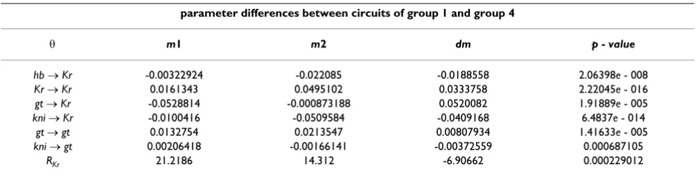
and causes the anterior hb dip. Also, tll activation by Gt is considerably decreased, leading to higher production of tll, which causes the tll-bump. Comparison of group 1 and 4 shows that Kr autoactivation is strong and repression by Gt is weak within group 4 (Table 2). This combination causes a local increased production of Kr on the domain where Gt is expressed. A consequence of the strong

autoactivation would be a higher level of Kr all along the A-P axis. This is prevented by increased repression through Hb and Kni. Also, the weaker production rate of Kr compensates for the strong autoactivation.

Pattern stability at later times

During gastrulation most of the gap domains, maternal bcd and cad disappear within 30 min. The anterior hb domain disappears rapidly during gastrulation [16], while posterior hb domain can still be detected for a few more hours until the end of germ band extension [17]. Central Kr domain decays rapidly after the onset of gastrulation [18,19]. Posterior gt domain disappears rapidly during gastrulation while the anterior domains persist for a few hours but change quite drastically and become involved in organ formation [20-22]. The entire kni domain and the posterior domain of tll disappear rapidly after gastru-lation [23,24].

The long-term dynamics of the circuits should show if the model is able to predict the disappearance of the gap gene domains, and provide information about the asymptotic stability of the model and potentially gives its attractors. The parameters were obtained by fitting the model to real data until gastrulation time. To study long term dynamics we simulated all circuits for an extended period (see Meth-ods, Additional file 1 and Additional files 2, 3, 4, 5 where long term dynamic movies are shown). We classified the behavior into the following groups:

1. stable patterns: 64 circuits, where tll and cad domains disappear completely in most cases. This group is com-posed of three sub-groups

(a) 9 circuits show a rudimentary gap gene pattern with all gene domains more or less well defined. (Figures 4-A, B).

(b) 27 circuits develop an uniform hb domain that covers the whole embryo. (Figures 4-C, D).

[image:5.612.54.557.99.226.2]

W_hbgt,W_gthb,W_tllgt

Table 2: Parameters' differences between circuits of group 1 and circuits of group 4.

parameter differences between circuits of group 1 and group 4

θ m1 m2 dm p - value

hb →Kr -0.00322924 -0.022085 -0.0188558 2.06398e - 008

Kr →Kr 0.0161343 0.0495102 0.0333758 2.22045e - 016

gt →Kr -0.0528814 -0.000873188 0.0520082 1.91889e - 005

kni →Kr -0.0100416 -0.0509584 -0.0409168 6.4837e - 014

gt →gt 0.0132754 0.0213547 0.00807934 1.41633e - 005

kni →gt 0.00206418 -0.00166141 -0.00372559 0.000687105

R_Kr 21.2186 14.312 -6.90662 0.000229012

(6)

Spatio-temporal surface plots showing the behavior of four different circuits at later times, and on the right the corresponding circuits

Figure 4

Spatio-temporal surface plots showing the behavior of four different circuits at later times, and on the right the corresponding circuits. Surface plots (panel a, c, e and g) represent the main types of patterns observed: a) Stable pat-tern with reminiscent patpat-tern (Group I). c) stable patpat-tern with a large hb suppressing all genes except gt (Group II). e) Oscilla-tory pattern where all genes except Tll oscillate (Group III). g) An oscillaOscilla-tory pattern where all genes except Kr and kni oscillate at the posterior (Group IV). In panel h the reduced circuit is shown. Only the connections that correlate with this par-ticular pattern are shown. In this circuit typical oscillatory motifs can be recognized. Edges between two vertices indicate acti-vation (green) or repression (red). The edge thickness is proportional to the absolute weight of the interaction.

time (min)

cad

35 54 74 92 0 68.1 200 400 600 800 1000 hb

35 54 74 92 Kr

35 54 74 92 gt

position (nucleus nr) 35 54 74 92

kni

35 54 74 92 tll

35 54 74 92

expression level 0 50 100 150 200 250

A hb cad

Kr gt kni tll bcd threshold B time (min) cad

35 54 74 92 0 68.1 200 400 600 800 1000 hb

35 54 74 92 Kr

35 54 74 92 gt

kni

35 54 74 92 tll

35 54 74 92

expression level 0 50 100 150 200 250 C cad hb Kr gt kni tll bcd threshold D time (min) cad

35 54 74 92 0 68.1 200 400 600 800 1000 1200 1400 1600 1800 2000 hb

35 54 74 92 Kr

35 54 74 92 gt

kni

35 54 74 92 tll

35 54 74 92

expression level 0 50 100 150 200 250

E hb cad

Kr gt kni tll bcd threshold F time (min) cad

35 54 74 92 0 68.1 200 400 600 800 1000 hb

35 54 74 92 Kr

35 54 74 92 gt

kni

35 54 74 92 tll

35 54 74 92

(7)

(c) 28 circuits show variable stable patterns with expand-ing or disappearexpand-ing domains.

2. Oscillatory patterns: (37 circuits) with the two sub-groups:

(a) 18 circuits with cad, hb, gt and tll showing posterior oscillations, while Kr and kni domains disappear. (Figures 4-E, F).

(b) 19 circuits where all genes oscillate but tll, which dis-appears (Figures 4-G, H).

We have compared parameters using T-tests and the aver-age circuit topology (see Table 3, 4 and 5). From Table 3, we see that the main difference between the two stable patterns is the strong hb autoactivation in the group with expanded hb. In some of the oscillatory circuits (Figure 4-H), we observed a basic motif composed of autoactivation and negative feedback loops. It can be shown theoretically that the minimal requirement for oscillations to occur in a two-gene network is that an activator activates its repres-sor and also itself. Nevertheless, the positive and negative feedback loops may be indirect and also the actual param-eter values may prevent the formation of oscillations even if the minimal requirement for oscillations is present. In the first oscillatory group we observe the basic motif for oscillation between Hb and Gt (Figure 5-H). In the data

we observe that the anterior hb peak slightly collapses, however it collapses more at the position of the anterior gt peak. In a number of circuits the fit to Hb is improved by repression of hb by Gt (group 2 cluster analysis). Almost all members of this group show oscillations. Hb in this group has an intermediate autoactivation (the group with strong autoactivation does not show oscillations) and Cad activates hb leading to constitutive activation of pos-terior hb. Next to the hb-gt oscillatory motif we see similar motifs with Tll. When negative feedback interactions are removed we observe that the corresponding gene does not oscillate any longer. Although the connections in these motifs are weak the behavior at later times is strongly affected.

Parameter correlations

From the two previous analyses and T-tests, we see that parameters differ from circuit to circuit leading to differ-ent behaviour. This might be a sign of overfitting, which can be determined by looking at the correlation matrix of all the parameters (Figure 5). Because of compensation mechanisms parameters may not be identifiable. Exam-ples of these are promoter and decay rates, which both scale the expression profile.

Furthermore, the input weights on a single gene can also compensate each other. If a positive input on a gene becomes stronger, increasing negative weights or decreas-ing positive weights can adjust for the increased total input, such that the total input on that gene is not altered much. However, these correlation patterns may be more intricate [see Additional file 1 for an extended correlation analysis].

Discussion

It seems difficult to determine which of the circuits have the "correct" topology. From the clustering of the gastru-lation profiles, we could have considered that only circuits without defects should be taken into account, but we see that it is not that trivial since the difference from circuit to circuit is not only based on the regulatory interaction type, but also their strength. None of the circuits predicted the disappearance of the gap genes during gastrulation, this

Table 3: Comparison of an average network with stable pattern formation(group I) against a network with a stable pattern and with expanded Hb domain (group II).

Network Differences

θ m1 m2 dm t

hb →hb 0.023993 0.020258 -0.00373504 0.0016962

bcd →kni 0.0448947 -0.0123351 -0.0572298 2.85189e - 006

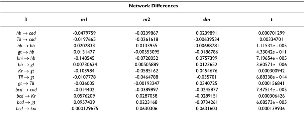
[image:7.612.56.553.615.710.2]

The table summarizes the list of parameters that are significantly different (mean mi, difference between mean dm and their p-value from the T-test t. The parameter difference found between Group I and II are the strength of hb autoactivation and the activation/ repression of kni by Bcd. [see Tab. S1 in Additional file 1, where networks diagrams are shown.]

Table 4: Comparison of an average network with a stable pattern group (group II) against oscillatory pattern (group III).

θ m1 m2 dm t

hb →hb 0.0202833 0.023993 0.00370971 0.000132337

kni →hb -0.148545 -0.0960403 0.0525049 0.000899982

hb →gt -0.00730634 0.000129385 0.00743572 0.00103439

bcd →kni -0.000129675 0.0448947 0.0450244 0.000589936

(8)

may be related to missing mechanisms like degradation of maternal genes. The long-term dynamics of the circuits show that the patterns converge to four main attractors. This difference in convergence may be explained by differ-ences in a few, but also the presence of certain motifs. More intriguing, one of the attractors resembles the gas-trulation pattern and circuits falling into this group have interactions more consistent with experimental evidence. Combined with the well defined parameters obtained from the correlation analysis [12], the following gap gene interactions consistent with literature were derived:

1. All the gap gene are activated by Cad.

2. All the gap gene but kni are activated by Bcd.

3. Hb, Kr gene have an auto-activation.

4. kni does not have a auto-repression, but certitude on auto-activation can not be deduced (strong correlation coefficient with most parameters)

5. Mutual repression between Hb and Kni

6. Mutual repression between Gt and Kr

These interactions are consistent with the regulatory mechanism proposed in [4] as well as those obtained in early literature [19-21, 25-29] and previous analysis [10]. Out of all the circuits, only 4 have a very good patterns and the mentioned regulatory interactions [circuits 20, 31, 82 and 101, see Additional file 6]. The alternative interactions proposed by the other circuits are a

conse-quence of overfitting, incomplete data and incomplete model structure.

For example biological evidence suggests that the anterior hb dip is caused by different early and late regulation mechanisms, which is not included in the current model, consequently the optimization predicts for many circuits suppression of hb by Gt to mimic this data feature. Fur-thermore the model tries to reproduce the experimentally observed decrease of cad by introducing negative feedback through the gap genes.

Jaeger et al. [4] suggested that the anterior shift of poste-rior domains after cycle 14A is caused by asymmetric repression of the gap genes. All the current circuits repro-duce the shift, but from the current analysis, it seems that the shift is not necessary a consequence of the asymmetric repression triggered by Hb. In many circuits we see that the shift of these domains continues to progress and leads to domain expansion or disappearance of other domains. The shift seems to correlate strongly with the posterior hb domain. The posterior hb domain develops later than the other domains, and represses gt, kni and Kr. In the circuits where the posterior hb domain continues to expand and in the end forms an almost uniform domain at steady state that covers the whole embryo; the anterior gt domain remains and Kr, kni, tll and cad all disappear. This phe-nomenon is caused by strong hb autoactivation, the other gap genes are not able to balance hb expression. The ante-rior gt domain remains because of maternal activation by Bcd and weak repression by Hb.

[image:8.612.54.551.99.287.2]

Schroder et al. [30] suggested that autoactivation is involved in maintenance of gap gene expression and

Table 5: Comparison of an average network of the two groups with oscillatory pattern (group III vs. group IV). 1

θ m1 m2 dm t

hb →cad -0.0479759 -0.0239867 0.0239891 0.000701299

Tll →cad -0.0197665 -0.0261618 -0.00639534 0.00334701

hb →hb 0.0202833 0.0133955 -0.00688781 1.11532e - 005

gt →hb 0.0131477 -0.00553095 -0.0186786 4.33042e - 011

kni →hb -0.148545 -0.0728052 0.0757399 7.19654e - 005

hb →gt -0.00730634 0.00505889 0.0123652 3.60571e - 006

Kr →gt -0.103984 -0.0585162 0.0454676 0.000300942

Tll →gt -0.0107778 -0.0464788 -0.035701 6.88338e - 014

gt →Tll -0.036005 -0.00193247 0.0340725 0.000156841

bcd →cad -0.014402 -0.0389897 -0.0245877 7.47514e - 005

bcd →Kr 0.0576209 0.0287058 -0.0289151 0.000306426

bcd →gt 0.0957429 0.0223168 -0.0734261 6.08573e - 005

bcd →kni -0.000129675 0.0630306 0.0631603 0.000139936

The table summarizes the list of parameters that are significantly different. All the parameters in the two groups have the predict the same

(9)

sharpening of gap domain boundaries [15]. Although this might be true, strong autoactivation also affects pattern stability later on during gastrulation, making it more dif-ficult for domains to fade. The inability of the circuits to predict transient expression suggests that either an addi-tional mechanism is missing in the model or that the opti-mization failed to capture the dynamics.

Competing interests

The authors declare that they have no competing interests.

Authors' contributions

All authors participated in the design of the study, and wrote the manuscript together. YF-N and MP conducted the analysis of data and simulations, and made the fig-ures. All authors read and approved the final manuscript.

Additional material

Additional file 1

Additional statistics. This file (GapGenePatternAnalysis BMCRN AddFile1) contains the material, which is not given in the paper due to the space limitations. In Section 1, models and methods are described. Section 2 gives a complete description of the simulated profiles. Section 3 complete the long term dynamics comparison with additional table-figures and Section 4 presents a complete correlation analysis.

Click here for file

[http://www.biomedcentral.com/content/supplementary/1756-0500-2-256-S1.PDF]

Additional file 2

Stable pattern with reminiscent pattern. Movies displaying the long term behaviour of a circuit showing a stable pattern with reminiscent gap gene pattern.

Click here for file

[http://www.biomedcentral.com/content/supplementary/1756-0500-2-256-S2.MP4]

[image:9.612.76.527.95.413.2]

Parameter correlation matrix

Figure 5

Parameter correlation matrix. Left: Matrix showing the pairwise correlation; the colour scale goes from intensive red (strong negative correlation) to bright green (positive correlation). The correlation matrix shows that there exist many pair wise correlations that tend to form clusters. Right: The absolute value of the correlation coefficients are used as a similarity measure to cluster the parameters, which is presented as a dendrogram. The parameters are sorted according to the dendro-gram.

1 0.5 0

similarity R−hb R−hb lambda−hb lambda−hb R−gt R−gt lambda−gt lambda−gt d−cad d−cad kni−>cad kni−>cad hb−>Kr hb−>Kr Kr−>Kr Kr−>Kr kni−>Kr kni−>Kr kni−>gt kni−>gt gt−>Kr gt−>Kr d−Kr d−Kr d−hb d−hb Kr−>hb Kr−>hb gt−>hb gt−>hb kni−>hb kni−>hb m−>hb m−>hb m−>kni m−>kni tll−>gt tll−>gt kni−>tll kni−>tll cad−>tll cad−>tll h−tll h−tll hb−>tll hb−>tll hb−>gt hb−>gt m−>gt m−>gt Kr−>gt Kr−>gt m−>Kr m−>Kr R−Kr R−Kr lambda−Kr lambda−Kr lambda−tll lambda−tll cad−>cad cad−>cad h−cad h−cad R−cad R−cad lambda−cad lambda−cad tll−>Kr tll−>Kr tll−>kni tll−>kni m−>tll m−>tll gt−>tll gt−>tll tll−>tll tll−>tll R−tll R−tll cad−>hb cad−>hb cad−>gt cad−>gt cad−>Kr cad−>Kr cad−>kni cad−>kni hb−>hb hb−>hb hb−>kni hb−>kni kni−>kni kni−>kni Kr−>kni Kr−>kni gt−>kni gt−>kni R−kni R−kni lambda−kni lambda−kni d−tll d−tll hb−>cad hb−>cad m−>cad m−>cad Kr−>cad Kr−>cad gt−>cad gt−>cad tll−>cad tll−>cad tll−>hb tll−>hb gt−>gt gt−>gt d−gt d−gt Kr−>tll Kr−>tll

d−kni d−kni

(10)

Acknowledgements

This work was supported by the Netherlands Organization for Scientific Research, project NWO-CLS 635.100.010 ("3d-RegNet: simulation of developmental regulatory networks", http://www.science.uva.nl/research/ scs/3D-RegNet) and by the EC (MORPHEX, NEST Contract No 043322). We used data from the FlyEx database http://flyex.ams.sunysb.edu/flyex/. We thank Dr. Johannes Jaeger for his wise suggestions.

References

1. Levine M: A systems view of Drosophila segmentation.

Genome Biol 2008, 9(2):207.

2. Sánchez L, Thieffry D: A logical analysis of the gap gene system.

Theor Biol 2001, 211:114-141.

3. Reinitz J, Sharp DH: Mechanism of eve stripe formation. Mech Dev 1995, 49(1-2):133-158.

4. Jaeger J, Surkova S, Blagov M, Janssens H, Kosman D, Kozlov KN, Myasnikova E, Vanario-Alonso CE, Samsonova M, Sharp DH, Reinitz J: Dynamic control of positional information in the early Dro-sophila embryo. Nature 2004, 430(6997):368-371.

5. Myasnikova E, Samsonova A, Kozlov K, Samsonova M, Reinitz J: Reg-istration of the expression patterns of Drosophila segmenta-tion genes by two independent methods. Bioinformatics 2001, 17:3-12.

6. Poustelnikova E, Pisarev A, Blagov M, Samsonova M, Reinitz J: A database for management of gene expression data in situ.

Bioinformatics 2004, 20(14):2212-2221.

7. Perkins TJ, Jaeger J, Reinitz J, Glass L: Reverse engineering the gap gene network of Drosophila melanogaster. PLoS Comput Biol

8. Fomekong-Nanfack Y, Kaandorp JA, Blom J: Efficient parameter estimation for spatio-temporal models of pattern formation: case study of Drosophila melanogaster. Bioinformatics 2007, 23(24):3356-3363.

9. Gutenkunst RN, Waterfall JJ, Casey FP, Brown KS, Myers CR, Sethna JP: Universally sloppy parameter sensitivities in systems biol-ogy models. PLoS Comput Biol 2007, 3(10):1871-1878.

10. Ashyraliyev M, Jaeger J, Blom JG: Parameter estimation and determinability analysis applied to Drosophila gap gene cir-cuits. BMC Systems Biology 2008, 2(83):.

11. George von Dassow EMM Eli Meir, Odell GM: The segment polar-ity network is a robust developmental module. Nature 2000, 406:188-192.

12. Jaqaman K, Danuser G: Linking data to models: data regression.

Nat Rev Mol Cell Biol 2006, 7(11):813-819.

13. Dougherty ER: Validation of Inference Procedures for Gene Regulatory Networks. Current Genomics 2007, 8:351-359. 14. Fomekong-Nanfack Y, Postma M, Kaandorp JA: Inferring

Dro-sophila gap gene regulatory network: a parameter sensitivity and perturbation analysis. BMC Systems Biology 2009, 3:94. 15. Jaeger J, Blagov M, Kosman D, Kozlov KN, Myasnikova E, Surkova S,

Vanario-Alonso CE, Samsonova M, Sharp DH, Reinitz J: Dynamical analysis of regulatory interactions in the gap gene system of Drosophila melanogaster. Genetics 2004, 167(4):1721-1737. 16. Tautz D, Lehmann R, Schnurch H, Schuh R, Seifert E, Kienlin A, Jones

K, Jaeckle H: Finger protein of novel structure encoded by hunchback, a second member of the gap class of Drosophila segmentation genes. Nature 1987, 327:383-389.

17. Tautz D: Regulation of the Drosophila segmentation gene hunchback by two maternal morphogenetic centres. Nature 1988, 332(6161):281-284.

18. Knipple DC, Seifert E, Rosenberg UB, Preiss A, Jaeckle H: Spatial and temporal patterns of Kruppel gene expression in early Drosophila embryos. Nature 1985, 317:40-44.

19. Gaul U, Jackle H: Pole region-dependent repression of the Dro-sophila gap gene Kruppel by maternal gene products. Cell 1987, 51(4):549-555.

20. Mohler J, Eldon ED, Pirrotta V: A novel spatial transcription pat-tern associated with the segmentation gene, giant, of Dro-sophila. The EMBO journal 1989, 8(5):1539-1548.

21. Eldon E, Pirrotta V: Interactions of the Drosophila gap gene giant with maternal and zygotic pattern-forming genes.

Development 1991, 111(2):367-378.

22. Kraut R, Levine M: Mutually repressive interactions between the gap genes giant and Kruppel define middle body regions of the Drosophila embryo. Development 1991, 111(2):611-621. 23. Rothe M, Nauber U, Jäckle H: Three hormone receptor-like

Drosophila genes encode an identical DNA-binding finger.

EMBO J 1989, 8(10):3087-94.

24. Pignoni F, Baldarelli RM, Steingrimsson E, Diaz RJ, Patapoutian A, Mer-riam JR, Lengyel JA: The Drosophila gene tailless is expressed at the embryonic termini and is a member of the steroid recep-tor superfamily. Cell 1990, 62:151-163.

25. Jackle H, Tautz D, Schuh R, Seifert E, Lehmann R: Cross-regulatory interactions among the gap genes of Drosophila. Nature 1986, 324(6098):668-670.

26. Harding K, Levine M: Gap genes define the limits of antennape-dia and bithorax gene expression during early development in Drosophila. The EMBO journal 1988, 7:205-214.

27. Struhl G, Johnston P, Lawrence PA: Control of Drosophila body pattern by the hunchback morphogen gradient. Cell 1992, 69(2):237-249.

28. Reinitz J, Levine M: Control of the initiation of homeotic gene expression by the gap genes giant and tailless in Drosophila.

Dev Biol 1990, 140:57-72.

29. Capovilla M, Eldon ED, Pirrotta V: The giant gene of Drosophila encodes a b-ZIP DNA-binding protein that regulates the expression of other segmentation gap genes. Development 1992, 114:99-112.

30. Schröder C, Tautz D, Seifert E, Jäckle H: Differential regulation of the two transcripts from the Drosophila gap segmentation gene hunchback. EMBO J 1988, 7(9):2881-2887.

Additional file 3

Stable pattern with a large hb suppressing all genes except gt contin-uously expanding to the left. Movies displaying the long term behaviour of a circuit showing a stable pattern with a large hb suppressing all genes except gt continuously expanding to the left.

Click here for file

Additional file 4

Oscillatory pattern where all genes except Tll oscillate. Movies display-ing the long term behaviour of a circuit showdisplay-ing an oscillatory pattern where all genes except Tll oscillate.

Click here for file

Additional file 5

Oscillatory pattern where all genes except Kr and kni oscillate at the posterior. Movies displaying the long term behaviour of a circuit showing an oscillatory pattern where all genes except Kr and kni oscillate at the pos-terior.

Click here for file

Additional file 6

Details parameters set of the 101 circuits. The data provided in the table contains a complete list of all the 101 circuits with their corresponding parameters.

Click here for file