CONVOLUTION SPLINE APPROXIMATIONS FOR TIME DOMAIN BOUNDARY INTEGRAL EQUATIONS
PENNY J. DAVIES AND DUGALD B DUNCAN
ABSTRACT. We introduce a new “convolution spline” temporal approximation of time domain boundary integral equations (TDBIEs). It shares some properties of convolu-tion quadrature (CQ) but, instead of being based on an underlying ODE solver, the approximation is explicitly con-structed in terms of compactly supported basis functions. This results in sparse system matrices and makes it com-putationally more efficient than using the linear multistep version of CQ for TDBIE time-stepping. We use a Volterra integral equation (VIE) to illustrate the derivation of this new approach: at time steptn=nhthe VIE solution is ap-proximated in a backwards-in-time manner in terms of basis functionsϕjbyu(tn−t)≈∑nj=0un−jϕj(t/h) fort∈[0, tn]. We show that using isogeometric B-splines of degree m≥1 on [0,∞) in this framework gives a second order accurate scheme, but cubic splines with the parabolic runout condi-tions at t = 0 are fourth order accurate. We establish a methodology for the stability analysis of VIEs and demon-strate that the new methods are stable for non-smooth ker-nels which are related to convergence analysis for TDBIEs, including the case of a Bessel function kernel oscillating at frequency O(1/h). Numerical results for VIEs and for TD-BIE problems on both open and closed surfaces confirm the theoretical predictions.
1. Introduction. Convolution quadrature (CQ) time-stepping for time-dependent boundary integral equations (TDBIEs) was first pro-posed and analyzed by Lubich in 1994 [31]. Since then, the inher-ent stability and ease of impleminher-entation of CQ (as compared to a full space-time Galerkin approximation) has made it a very popular
2010 AMSMathematics subject classification. Primary 65R20, 65M12.
Keywords and phrases. Convolution quadrature, Volterra integral equations, time dependent boundary integral equations.
This work was supported by the UK Engineering and Physical Sciences Re-search Council grant EP/G036136/1 for the Centre for Numerical Algorithms and Intelligent Software.
Received by the editors on June 21, 2013, and in revised form on March 12, 2014.
DOI:10.1216/JIE-2014-26-3-369 Copyright⃝c2014 Rocky Mountain Mathematics Consortium
choice for TDBIE problems–a search on “convolution quadrature,”
“boundary” in the Thomson Reuters Web of Science database yields
nearly 200 hits. Unfortunately there is a drawback: the effective sup-port of the time basis functions ϕj(t) which underpin CQ increases
withj, and this increases the computational complexity of the solution algorithm. Here we describe a new “convolution spline” approxima-tion framework which shares some properties with CQ but is explicitly constructed in terms of compactly supported basis functions which are (mainly) translates; this makes it easy to implement and computation-ally efficient. We apply it to the TDBIE problem
(1.1) 1
4π ∫
Γ
u(⃗x′, t−|⃗x′−⃗x|)
|⃗x′−⃗x| d⃗x
′ =a(⃗x, t) for⃗x∈Γ, t >0
foru; this is the single layer potential equation for acoustic scattering from the surface Γ⊂R3 with zero Dirichlet boundary conditions and (known) incident field−a(⃗x, t), which is equivalent to
∫ t
0 ∫
Γ
k(⃗x′−⃗x, t−t′)u(⃗x′, t′)d⃗x′dt′=a(⃗x, t) fork(⃗z, t) =δ(t− |⃗z|) 4π|⃗z| .
We use the convolution-kernel Volterra integral equation (VIE)
(1.2)
∫ t
0
K(t′)u(t−t′)dt′ =a(t), t∈[0, T]
to illustrate the derivation of the new approximation method and its convergence and stability properties. However, the focus of the paper is not on deriving new methods for VIEs (of which there are already very many), but on using the insight gained from VIEs to derive new methods which have good properties for TDBIEs.
1.1. Properties of TDBIE approximations. Designing a good approximation scheme for the TDBIE (1.1) is nontrivial; challenges include ensuring that it is numerically stable, it is not prohibitively hard to implement for a given scattering surface Γ, and its computational complexity is not infeasibly high. We begin by briefly summarizing the pros and cons of some of the main approaches (see also[9, 22]).
stability of the method relies on all the integrals being evaluated very accurately (the key insight on how to do this was provided by Terrasse [39]). In practice this involves converting five-dimensional volume in-tegrals over irregular (non-polygonal) sub-regions of Γ×Γ×[0, T] to surface integrals which are then evaluated using high precision quadra-ture and is extremely complicated to successfully implement in practice, even for relatively simple Γ. Collocation schemes for (1.1) are far more straightforward to implement, but there is little rigorous convergence analysis for them, and numerical instability is often an issue. As noted above, methods which use a Galerkin approximation in space and CQ in time have obvious attractions: they are based on rigorous theoretical analysis[1, 31](see also[16]for some new bounds) and are relatively straightforward to implement. They are also inherently far more sta-ble than those which use Galerkin or collocation time approximations (Lubich showed in [31]that the CQ method remains stable when the inner product integrals are approximated), but unfortunately the dis-advantage this time is higher computational complexity.
All three approaches approximate (1.1) as a convolution sum of the form∑nj=0QjUn−j
=an, which is rearranged to give the time-stepping
scheme
(1.3) Q0Un=an−
n
∑
j=1
QjUn−j
forUn ∈RNS, the representation of the spatial approximation ofuat or
near timetn =n h, where the right-hand side vectoran is derived from
a(⃗x, t). In the case of both Galerkin and collocation approximations the matricesQj∈RNS×NS are sparse–the number of nonzero elements
per row of matrix Qj is O(min{j, N1/2
S }). In particular, this means
that (1.3) can be solved in O(NS3/2) operations once the right-hand side is known, and the overall computational complexity to obtain the approximate solution up to time NTh is O(min{NT3NS, NT2N
3/2
S })
operations. For these hyperbolic problems, it is usual to use a timestep h commensurate with the side ∆x of a typical space mesh element, and in this case NT ≈ N and NS ≈ N2 for N = 1/∆x, and the
developed by Michielssen and co-workers [17, 18, 29] reduces the complexity toO(N3 log2N).
Using CQ in time results in a solution algorithm (1.3) in which the matrices Qj are dense, because the underlying basis functions are
global (see, e.g., Section 2 below, or [2, 23] for more details), which increases the computational complexity to O(N2
SNT2). The issue is
not solving (1.3) for Un (which can typically be done efficiently by approximatingQ0 appropriately), but in performing the matrix-vector products needed to calculate the right-hand side. Lubich explains that the technique of [24]can be used to reduce the overall complexity to
O(N2
SNT log2NT), i.e.,O(N5log2N). A cut-off strategy for replacing
small matrix entries by zero is described and analyzed in[23], and this reduces the storage costs of the method. This is combined with panel clustering in[26]to further reduce the storage costs. However, because the effective support of the time basis functions increases with the index (see Figure 2 or [13, Figure 2.2]), the computational complexity is a factor of√Nhigher than that for approximations which use local basis functions.
CQ methods which are based on underlying Runge-Kutta ODE solvers have also been developed and analyzed for TDBIEs [3, 4]. There are several advantages of these methods over linear multistep CQ methods: the basis functions are more highly concentrated[2, Figures 1, 2], which makes sparsifying the Qj matrices more straightforward; and higher order accurate methods in time are possible. Banjai[2]uses this approach to develop a practical, parallelizable solution algorithm for (1.1) which he illustrates with a number of realistic large-scale numerical examples.
1.2. New convolution spline methods. The Qj system matrices
in (1.3) for our new method have the same sparsity pattern as for the Galerkin or collocation approximations described above, and so it is considerably more efficient (both to set up by calculating the system matrices, and to run) than using the linear multistep version of CQ. Our method gives a TDBIE solution scheme whose overall complexity is O(min{N3
TNS, NT2N
3/2
S }) = O(N
5) operations (and which could
We derive the new approximation as a solution method for the VIE (1.2), with u approximated in terms of B-spline basis functions in a backwards-in-time framework. Our initial approach is to use isogeometric B-splines of degreemon [0,∞). There can be advantages in using higher order values ofm even though the formal convergence rate of this scheme for a smooth VIE problem is limited to second order (because it is based on quasi-interpolation by the Schoenberg B-spline operator). For example, as noted in[36], using smooth temporal basis functions greatly simplifies approximating the integrals in (1.1). We also consider cubic B-splines with the parabolic runout condition at t= 0 and show that these are fourth order accurate. We carefully test out the new methods on (1.2), establishing formal convergence, and examining the behavior for kernels which mimic some of the important properties of TDBIE problems, such as discontinuous step-function kernels (see, e.g., [37]). Another important test problem is obtained from taking the spatial Fourier transform of (1.1) at frequency⃗ω∈R2 when Γ =R2. This is
(1.4)
∫ t
0
J0(ωt′)bu(⃗ω, t−t′)dt′ = 2ba(⃗ω, t),
where ω = |⃗ω| and J0 is the first kind Bessel function of order zero. As noted in[10], instabilities of approximation schemes for (1.1) are typically exhibited at the highest spatial frequency which can be represented on the mesh. Hence, it is important to ensure that any prototype numerical scheme for time-stepping (1.1) is stable for (1.4) at values ofω=O(1/h) (assumingh≈∆x).
1.3. Outline. Section 2 contains an alternative derivation of Lubich’s [30]CQ method for (1.2) in terms of basis functions which have the sum to unity property (2.12). The new convolution spline approximation of (1.2) is described in Section 3 in terms of basis functions which have compact support and are (essentially) all translates, and we give suffi-cient conditions for this approximation to be stable. We consider the case in which the basis functions aremth degree isogeometric B-splines on [0,∞) in Section 4, showing how Laplace transform techniques can be used to prove the stability of this approximation of (1.2) for several different test kernels, and demonstrating second order convergence for (1.2) whenKand asatisfy
for suitabled≥0. Under these assumptions, equation (1.2) possesses a unique solutionu∈Cd[0, T], e.g., see[6, Theorem 2.1.9].
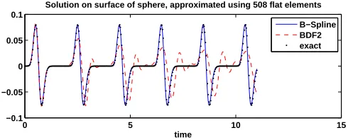
In Section 5, we consider a cubic convolution spline basis which is modified neart= 0 to satisfy the parabolic runout conditions and show that this gives a far more stable approximation of (1.2) which is fourth order convergent. Numerical tests show that it achieves fourth order accuracy even for a discontinuous kernel. We present numerical test results for TDBIEs in Section 6 which use a Galerkin approximation in space (based on triangular piecewise constant elements), and the new cubic convolution spline basis in time, for both open and closed surfaces Γ. These show that the new scheme performs far better than CQ based on BDF2–it is both more accurate and more efficient.
The TDBIE test problems are similar to those considered in [13] which use the convolution-in-time framework with non-polynomial (global) basis functions, but the modified B-spline basis functions give a more accurate temporal approximation. We note that the time-stepping schemes of [13]rely on the theoretical framework developed in Sections 2–3 of the present work.
2. CQ based on linear multistep methods for (1.2). We begin by outlining Lubich’s derivation [30] of the CQ method for (1.2) in order to show how it can be reinterpreted in terms of CQ basis functions. For simplicity we restrict attention to the case for which the extension of the solution u by zero to the negative real axis is in Cd(−∞, T] (otherwise the CQ method needs to be ‘corrected’ as
described in [30, Section 3] in order to attain optimal convergence). This is guaranteed by requiring
(2.1) a(p)(0) = 0 forp= 0 :d+ 1
becauseu(p)(0) =a(p+1)(0)−∑p−1
ℓ=0K
(p−ℓ)(0)u(ℓ)(0). We also assume
2.1. Lubich’s CQ method. We follow Lubich [30] and substitute the Laplace inversion formula forK(s) into (1.2) to obtain
(2.2) a(t) = 1
2πi ∫
γ
K(s)y(t, s)ds,
where γis an infinite contour within the region of analyticity of K(s) and
y(t, s) = ∫ t
0
est′u(t−t′)dt′.
Treating the Laplace variablesas a parameter,y(t) solves the ODE:
(2.3) y˙(t) =s y(t) +u(t), y(0) = 0,
and this is approximated by thek-step (k≤d) linear multistep method with timesteph
(2.4)
k
∑
j=0
αjyn+j−k =h k
∑
j=0
βjfn+j−k,
wheretn=nh,yn≈y(tn) andfn =s yn+u(tn). The starting values
are y−k = · · ·y−1 = 0 because of the assumption (2.1). Multiplying (2.4) byξnand summing overn(forξ∈Cfor which the sum converges) gives
( δ(ξ)
h −s )∑∞
n=0
ynξn=
∞
∑
n=0
u(tn)ξn,
where
δ(ξ) =
k
∑
j=0 αjξk−j
/∑k
j=0 βjξk−j
is the symbol of (2.4). Hence,ynis the coefficient ofξnin the expansion
of (δ(ξ)/h−s)−1∑∞
k=0u(tk)ξk. Substitutingynfory(tn) in (2.2) shows
thata(tn) is approximated by the coefficient ofξn in
1 2π i
∫
γ
( δ(ξ)
h −s )−1
K(s)ds
∞
∑
k=0
u(tk)ξk =K(δ(ξ)/h)
∞
∑
k=0
using Cauchy’s integral formula. Hence, defining the CQ weights qk=qk(h) to be the coefficients in the expansion
(2.5) K(δ(ξ)/h) = ∞
∑
k=0 qkξk
gives the CQ approximation of (1.2)
(2.6) a(tn) =
n
∑
j=0
qjun−j.
This can be rearranged to give the time-stepping approximate solution un≈u(tn)
(2.7) un=
1 q0
( a(tn)−
n−1 ∑
j=1 qjun−j
)
forn≥1,
since, by assumption,u0=u(0) = 0.
2.2. Derivation of CQ in terms of basis functions. The CQ approximation scheme (2.6) for the VIE (1.2) is defined solely in terms of the weights qk. But, if CQ is used to time-step a TDBIE,
then the approximation involves CQ basis functions, see e.g., [2, 23, 32]. However, we are not aware of a general interpretation of CQ approximation schemes for (1.2) in terms of basis functions. As well as yielding some interesting observations, this also gives the framework which we use for the derivation of our convolution spline methods in Sections 4–5.
Att=tn :=nh, (1.2) can be written as
(2.8) a(tn) =
∫ ∞
0
K(t′)u(tn−t′)dt′,
because u(t) = 0 for t ≤ 0. We show below that the standard CQ method is equivalent to approximatinguin (2.8) by
(2.9) u(tn−t′)≈ n
∑
j=0
un−jϕj(t′/h) fort′ ≥0,
where ϕj are basis functions, i.e., the approximation at tn is Un(t) =
∑n
onn, i.e., CQ isfundamentally different from a standard finite-element type approximation in which an unknown coefficient is always associ-ated with the same basis function.
Substituting (2.9) into (2.8) and comparing the resulting expression with (2.6) gives the relationship between the standard CQ weights and basis functions:
(2.10) qj=
∫ ∞
0
K(t)ϕj(t/h)dt .
Comparing this with the standard CQ definition of qj in (2.5) gives
(see[2, Equation (3.1)])
(2.11) e−δ(ξ)t= ∞
∑
j=0
ϕj(t)ξj.
An immediate consequence is that the basis functions satisfy the sum to unity property
(2.12)
∞
∑
j=0
ϕj(t) = 1,
provided the underlying multistep ODE solver is consistent, because in this case δ(1) = 0. This new observation is a crucial property which we use in Section 3.
2.3. CQ basis functions for LMMs. Explicit formulae for the ϕj(t) based on BDF1-2 have been used for TDBIE approximations
[23, 32]. The formula for BDF1 is given in [32], and in this case, ϕj(t) = e−ttj/j!, i.e., they are Erlang functions, used in statistics as
probability density functions and satisfyϕj(t)≥0 and
∫∞
0 ϕj(t)dt= 1. The derivation for BDF2 is more complicated, and the explicit formula
ϕj(t) =
1 j!Hj(
√
2t) (
t 2
)j/2 e−3t/2
is given in [23], where Hj is the jth Hermite polynomial. Note that
the properties ofHj imply thatϕj(t) involves ajth degree polynomial
and an exponential int with no fractional powers oft.
for (2.3), although this may not be easy in practice. For the trapezoidal ruleδ(ξ) = 2 (1−ξ)/(1+ξ)[2],and (2.11) is∑∞j=0ϕj(t)ξj=e−2tf(ξ),
wheref(ξ) = exp(4t/(1 +ξ)). This givesf(ξ) =∑∞j=0fjξj where
fj=
1 j!
dj
dξjf(ξ)
ξ=0
= 1
j!(4t)j
dj
dzj e
−1/z
z=1/(4t)
using the change of variables z = (1 + ξ)/(4t). It follows from [33, equation 18.5.6] that fj = (−1)je−4tL−j1(4t), where L
α j(x) is
a Laguerre polynomial. The identity L−j1(x) = Lj(x)−Lj−1(x)[20, equations 8.971–5] gives the trapezoidal rule basis functions ϕj(t) =
(−1)j{ℓ
j(4t)−ℓj−1(4t)}, whereℓj(x) =e−x/2Lj(x) is thejth Laguerre
function. They are oscillatory but do satisfy∫0∞ϕj(t)dt= 1. The low
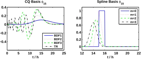
order basis functions are shown in Figure 1 (see also[2, Figure 1]and [32,Figure 4]). Figure 2 shows how the CQ basis functions spread out as j increases; this increases the number of non-zero entries in the Qj
matrices of (1.3) and makes CQ time-stepping less efficient.
0 5 10 15 20 25
−0.4 −0.2 0 0.2 0.4
t / h CQ Basis φ15
BDF1 BDF2 BDF3 TR
12 14 16 18 20 22
0 0.2 0.4 0.6 0.8 1
t / h Spline Basis φ
15
[image:10.432.104.346.333.437.2]m=0 m=1 m=2 m=3
Figure 1. Typical CQ and spline basis functions. See subsections 2.3 and 4.1 for details.
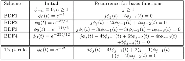
The direct approach appears intractible for more complicated schemes (even for BDF3), and recurrence relations for the basis functions are given in [32, subsection 3.2]. They can be compactly derived by for-mally differentiating the generating function (2.11) with respect to ξ to get
∞
∑
j=1
jϕj(t)ξj−1+tδ′(ξ)
∞
∑
j=0
0 5 10 15 20 25 30 35 40 45 50 10−10
10−5 100
t Size of the basis functions φ
5(t) and φ25(t)
[image:11.432.101.347.110.213.2] [image:11.432.74.377.275.376.2]φ5 φ25
|B−spline| |BDF2|
Figure 2. Basis functionsϕ5(t) andϕ25(t) for CQ (BDF2) compared with cubic splines (from Sec. 5). The effective support of the CQ basis functions
ϕj(t) increases withj.
Scheme Initial Recurrence for basis functions
ϕ−n≡0, n≥1 j≥1 BDF1 ϕ0(t) =e−t jϕj(t)−tϕj−1(t) = 0
BDF2 ϕ0(t) =e−3t/2 jϕj(t)−2tϕj−1(t) +tϕj−2(t) = 0
BDF3 ϕ0(t) =e−11t/6 jϕj(t)−3tϕj−1(t) + 3tϕj−2(t)−tϕj−3(t) = 0 BDF4 ϕ0(t) =e−25t/12 jϕj(t)−4tϕj−1(t) + 6tϕj−2(t)−4tϕj−3(t)
+tϕj−4(t) = 0
Trap. rule ϕ0(t) =e−2t jϕj(t)−4tϕj−1(t) + 2(j−1)ϕj−1(t)
+(j−2)ϕj−2(t) = 0 Table 1. Recurrence relations for the CQ basis functions.
and then collecting terms in ξ. The initial conditions are ϕn(t) ≡ 0
for n < 0, and the first term of the Taylor expansion of (2.11) gives ϕ0(t) = e−δ(0)t = e−δ0t. Recurrence relations for BDF1–4 and the trapezoidal rule are given in Table 1.
3. Convolution spline approach. As discussed in Section 1, basis functions with global support (such as those described above) give rise to dense matrices Qj in the TDBIE scheme (1.3), and this has
in Sections 4–5. This new approach gives sparse system matrices when used to time-step TDBIEs, and results are presented in Section 6. It also provides the underpinning theoretical framework for the TDBIE time-stepping approximations of[13].
3.1. Construction of a convolution spline scheme for (1.2). We consider approximations of the form (2.9), but where all the basis functions ϕj have compact support of width O(h) and almost all are
translates of a standard, compactly supported basis functionϕm, i.e.,
(3.1) ϕj(t/h) =ϕm(t/h+m−j) forj ≥m.
When the basis functions are splines, then m is also equal to the polynomial degree.
Property (3.1) means that the approximationU(tn−t)≈u(tn−t)
has the form
(3.2) U(tn−t) = m∑−1
j=0 vn−jϕj
( t h
) +
n
∑
j=m
vn−jϕm
( t
h+m−j )
for t ≥0, where vj approximates u(t) fort near (but not necessarily
at)tj, and a sum is defined to be zero if its upper index is less than its
lower index. Note that when all the ϕj are translates (as happens for
piecewise constant or linear approximations), thenϕn−k(n−s)≡ϕk(s)
and the convolution-in-time representation (2.9) fits into a standard finite element framework.
Substituting the approximation (3.2) into the integral equation (1.2) and collocating at each time level as described in subsection 2.2 gives
(3.3)
n
∑
j=0
qjvn−j =a(tn)
for n = 0 : N where the weights qj are defined by (2.10). The
unknown coefficients {vj}N
j=0 are then found by time marching as in (2.7). An alternative expression which is useful for analysis is q0vn =
∑n
j=0pja(tn−j) for n ≥ 1, where the stability coefficientspn
are defined recursively by
(3.4) p0= 1, pn= −
1 q0
n
∑
j=1
3.2. Stability of (3.3). For TDBIE applications and analysis (see, e.g., [12]), we require the scheme (3.3) to be stable in the following sense, independent of the input functiona(t).
Definition 3.1(Stability). The scheme (3.3) is said to be stable when the impulse response sequence {pn}defined by (3.4) satisfies |pn| ≤C for allnsuch thatnh≤T, where the constantC is independent ofh.
This is weaker than BIBO (bounded input bounded output) stability in the signal processing literature (see, e.g., [35]), which requires boundedness of the absolute sum∑∞n=0|pn|<∞.
Stability properties of the scheme (3.3) can be established by using the Z-transform, defined as follows.
Definition 3.2. The Z-transform of a sequence{fn}∞n=0is the function F given by
(3.5) F(ξ) =Z{fn}(ξ) = ∞
∑
n=0 fnξn
whereξ∈Cwith |ξ| ≤1 is such that the sum converges.
The scheme (3.3) is a convolution sum, and its Z-transform is
(3.6) Q(ξ)V(ξ) =A(ξ),
where
(3.7) Q(ξ) =
∞
∑
j=0 ξj
∫ ∞
0
K(t)ϕj(t/h)dt
and we takean =a(tn). Thepncoefficients satisfy
∑n
j=0qjpn−j= 0 for
n≥1, and whenn= 0 this “sum” is equal toq0(becausep0= 1), and so the Z-transform of (3.4) is Q(ξ)P(ξ) =q0, giving P(ξ) =q0/Q(ξ). We now state a sufficient condition for stability whenQ(ξ) is a rational function.
Theorem 3.1 (Root condition for stability). If the Z-transformQ(ξ)
following for any constantc≥0 (independent of h): |ξk| ≥1/(1 +ch)
and any with1/(1 +ch)≤ |ξk| ≤1are simple.
Simple roots with|ξk|= 1/(1 +ch) make a bounded contribution to
pn asnincreases by the standard result
|ξk|−n= (1 +ch)n≤ecT
for tn ≤ T, but roots of this size with multiplicity µ ≥2 contribute
terms which grow likenµ−1and hence violate the stability definition.
Remark. Although this result is a variant of the root condition
familiar (after the change of variable z = 1/ξ) from zero stability analysis of numerical methods for ODEs, we note that it does not appear to have previously been derived or used to determine the stability of VIE schemes.
Verifying the stability condition directly or via the root condition above for a general approximation scheme for (1.2) may be very com-plicated. But, as we show below, schemes with the translate property (3.1) can be tackled within the framework of Laplace transforms origi-nally introduced for CQ, and this approach gives a way to extend the scope of stability analysis to a far broader range of kernel functions.
Substituting the Laplace inversion formula forK into (2.1) gives
qj =
h 2πi
∫
γ
K(s) Φj(−sh)ds,
where Φj(s) is the Laplace transform ofϕj. Hence, the approximation
scheme (3.3) can be written as
(3.8) a(tn) =
1 2πi
∫
γ
K(s)yn(sh)ds
where
yn(sh) =h n
∑
j=0
vn−jΦj(−sh).
We note thatynplays the same role here that the approximate solution
The translate property (3.1) and the compact support ofϕmimply
Φj(−sh) =esh(j−m)Φm(−sh) forj≥m,
and so
yn(sh)−eshyn−1(sh) =hvnΦ0(−sh)
+h
m
∑
j=1 vn−j
(
Φj(−sh)−eshΦj−1(−sh) )
,
(usingvj ≡0,j≤0). Taking the Z-transform of this expression gives
Y(ξ, sh) =hB(ξ, sh)V(ξ)/(1−eshξ)
whenξ̸=e−sh, where
(3.9) B(ξ, sh) = Φ0(−sh) +
m
∑
j=1 [
Φj(−sh)−eshΦj−1(−sh) ]
ξj.
It hence follows from (3.8) that
A(ξ) =V(ξ) h 2πi
∫
γ
K(s) (
B(ξ, sh) 1−eshξ
) ds
and comparison with (3.6) yields the alternative representation for the Z-transform of the weightsqj:
(3.10) Q(ξ) = h 2πi
∫
γ
K(s) (
B(ξ, sh) 1−eshξ
) ds.
The expression B(ξ, sh)/(1−eshξ) plays a role similar to that of
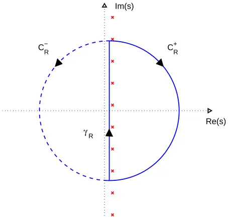
(δ(ξ)/h−s)−1 in standard CQ analysis, and it is the key quantity in determining whether the scheme is stable or not. Unfortunately, it has a more complicated structure: it has an infinite vertical line of simple poles ats=sk fork∈Z, where
(3.11) sk:=
1
h(−ln|ξ| −iArg (ξ) +i2πk)
and the principal argument Arg (ξ) ∈ (−π, π]. Note that, if |ξ| <1, then Re (sk)>0.
C+
R
C−
R
γR Re(s)
[image:16.432.112.339.109.328.2]Im(s)
Figure 3. The left and right D-contours of radiusRused for the stability and Z-transform calculations. The crosses are the poles (3.11) and the vertical line of length (approximately) 2RisγR.
taking the limit R→ ∞and settingγ = limR→∞γR. Using the right
contour gives
Q(ξ) = ∞
∑
k=−∞
K(sk)B(ξ, skh)− lim R→∞
h 2πi
∫
CR+
K(s) (
B(ξ, sh) 1−eshξ
) ds.
The integral roundCR+does not necessarily vanish asR→ ∞since, for some basis functions (including higher order B-splines), the quantity
B(ξ, sh) 1−eshξ =O(e
csh)
result
Q(ξ) =h∑
j
lim
s→κj
(
(s−κj)B(ξ, sh)
1−eshξ K(s)
)
− lim
R→∞
h 2πi
∫
CR−
K(s) (
B(ξ, sh) 1−eshξ
) ds .
The asymptotic behavior of the integralCR− as R→ ∞is determined primarily by K(s). The extension of this left contour approach to poles with higher multiplicity is straightforward. We illustrate the use of these formulae in subsection 4.2 for various kernelsKwhen the basis functions are B-splines.
4. B-spline basis functions for (1.2). We now illustrate the the-oretical framework introduced in Section 3 for basis functionsϕjwhich
are B-splines on [0,∞). We begin by listing some general properties of B-splines which are needed in the subsequent analysis and then ex-amining the stability of the convolution spline approximation of (1.2) for different example kernels. We also prove that the approximation given by (3.3) converges to the solutionu of (1.2) for general smooth a and K. The convergence rate is at most second order, no matter how high the polynomial degree, because quasi-interpolation by the Schoenberg B-spline operator is at most O(h2) [14]. However, a sim-ple modification of the B-spline basis neart= 0 can give higher order stable approximations of (1.2), and this is analyzed for the cubic case in Section 5.
4.1. Notation and properties. We now look in detail at the approx-imation (3.2) when the basis functions are (iso-geometric) B-splines of polynomial degree mbased on the uniformly spaced nodes (or knots) tj = j h forj ≥0. It is necessary for the B-spline basis functions to
have the sum to unity property (2.12) in the whole interval [0,∞), and we introduce m new knotstj = 0 for j =−m :−1. The mth degree
B-splines are bm
j (t) for j ≥ −m, and B-splines of degree m > 0 are
recursively defined in terms of those of lower degree as follows, using the convention thatbm
j (t)≡0 forj <−m.
Definition 4.1. [14]Whenm= 0,
b0j(t) = {
Ifm >0, then
bmj (t) = (
t−tj
tj+m−tj
)
bmj −1(t) + (
tj+m+1−t tj+m+1−tj+1
) bmj+1−1(t)
where the convention is that 0/0 is interpreted as 0.
Throughout this section, we shall use basis functions
(4.1) ϕj(t/h) =bmj−m(t) forj≥0.
Note that the spline degree m is also the translate parameter from (3.1).
We make use of several B-spline properties in Section 4 (see, for example, standard references such as [14, 38]), which we list here for convenience.
B-spline properties.
P1 Compact support. bmj (t) = 0 outwith [tj, tj+m+1), and bm
j (tj) = 0 unless j=−m.
P2 Translate property. If j ≥ 0, then bm
j (t) = bm(t/h−j),
where the functionsbmare defined recursively:
b0(τ) = {
1 ifτ∈[0,1), 0 otherwise,
and ifm≥1:
bm(τ) = τ mb
m−1(τ) +m+ 1−τ
m b
m−1(τ−1).
It follows thatϕj(τ) =bm(τ+m−j) forj≥m.
P3 Sum to unity. ∑∞j=−mbm
j (t) = 1 for allt≥0.
P4 Moments. ∫ tj+1
tj−m
bmj−m(t)dt=tj+1−tj−m m+ 1
and ∫ tj+1
tj−m
t bmj−m(t)dt= tj+1−tj−m (m+ 1)(m+ 2)
m∑+1
k=0
P5 Shoenberg quasi-interpolation. Suppose thatm≥1, and set tm
j = [h(m+j) (m+j+ 1)]/2m for j = −m : −1 and
tm
j =tj+(m+1)/2 for j ≥ 0. Then ∑∞
j=−mt m
j bmj (t) = t when
t≥0.
It follows from properties P1, P3 and P5 above that
(4.2) f(t) =
∞
∑
j=−m
f(tmj )bjm(t) +O(h2)
for anyf ∈C2[0,∞), and iff ∈Cp+1[0,∞) forp≥2 andt∈[tℓ, tℓ+1) for someℓ≥0, then
(4.3) f(t)−
ℓ
∑
j=ℓ−m
f(tmj )bmj (t) =
p
∑
k=2 f(k)(t
ℓ)
k!
×
[
(t−tℓ)k− ℓ
∑
j=ℓ−m
( tmj −tℓ
)k
bmj (t) ]
+O(hp+1).
It follows from P1 that the CQ weights are
(4.4) qj=
∫ tj+1
tj−m
K(t)bmj−m(t)dt.
The convergence analysis relies crucially on knowing the values of the weights whenK is a constant, and this follows immediately from P4: whenK≡1, the weightsqj of (4.4) are given by
qj
h = {
(j+ 1)/(m+ 1) forj= 0 :m−1
1 ifj≥m.
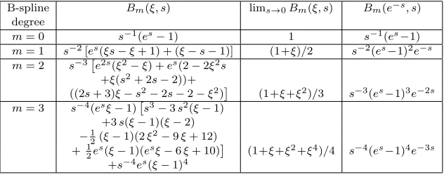
4.2. Stability results for convolution B-splines. We now use the theoretical framework introduced in Section 3 to examine the stability of the convolution B-spline approximation of (1.2) for different example kernels which capture some of the important properties of TDBIE problems. These are: K(t) equal to a constant, a step function and the highly oscillatory kernels K(t) = J0(ωt) or cos(ωt), where ω can be of the order of 1/h. We use Bm(ξ, sh) to denote the function
defined by (3.9) for the degreembasis functions, andQm(ξ) to denote
more complicated but are easily computed in a standard algebraic manipulation package.
In three of the cases Qm(ξ) is a rational function in ξ and
Theo-rem 3.1 can be used to determine stability. The Bessel function case is more complicated, and stability is determined from the Z-transform inversion formula by bounding the coefficientspnof (3.4) directly. Note
that this bound is independent of nand so is a practically useful sta-bility result, in contrast with the (essentially) uncheckable hypotheses needed in[11].
B-spline Bm(ξ, s) lims→0Bm(ξ, s) Bm(e−s, s) degree
m= 0 s−1(es−1) 1 s−1(es−1) m= 1 s−2[es(ξs−ξ+ 1) + (ξ−s−1)] (1+ξ)/2 s−2(es−1)2e−s m= 2 s−3[e2s(ξ2−ξ) +es(2−2ξ2s
+ξ(s2+ 2s−2))+
((2s+ 3)ξ−s2−2s−2−ξ2)] (1+ξ+ξ2)/3 s−3(es−1)3e−2s m= 3 s−4(esξ−1)[s3−3s2(ξ−1)
+3s(ξ−1)(ξ−2)
−1
2(ξ−1)(2ξ
2−9ξ+ 12)
[image:20.432.72.388.235.361.2]+ 12es(ξ−1)(esξ−6ξ+ 10)] (1+ξ+ξ2+ξ4)/4 s−4(es−1)4e−3s +s−4es(ξ−1)4
Table 2. The functionBm(ξ, s) form= 0 : 3. (See text for details.)
4.2.1. Constant kernel: K(t) = 1, transform K(s) = 1/s. Integrating (3.10) round the left contour in Figure 3 gives
(4.5) Qm(ξ) =hlim s→0
Bm(ξ, sh)
1−eshξ =
h(1−ξm+1) (m+ 1)(1−ξ)2.
The functionQmhasmsimple roots on the unit circle, and stability of
the approximation then follows from Theorem 3.1. (Note that stability also follows from the convergence result of subsection 4.3.)
described in [37] for more general scattering from spheres involving higher spatial harmonics.
We assume that the durationLis independent ofhand denote the integer part ofL/hbyM, i.e., whenhis sufficiently small,L= (M+r)h for integerM > mandr∈[0,1). It is simplest to work with the explicit Z-transform formula (3.5) using the weights given in (4.4). Results for m= 0 : 3 are summarized below.
Case m=0.
Q0(ξ) h =r ξ
M+ M∑−1
n=0
ξn= 1 ξ−1
(
r ξM+1+ (1−r)ξM−1).
Whenr∈(0,1), it can be shown that the M rootsξj of Q0 satisfy |ξj|>1 forj = 1 : M, and when r= 0 there are M −1 simple roots ξj= exp(i2πj/M) forj = 1 :M−1. Hence, Theorem 3.1 implies that
them= 0 scheme is stable for allL.
Case m=1. We have
Q1(ξ) =h 2
1 1−ξ
(
1 +ξ−ξMg),
withg(r, ξ) =ξ+ (1−r+rξ)2andr∈[0,1). Using the definition (3.4) and formal power series expansion for smallξgives
P1(ξ) = h 2Q1(ξ) =
1−ξ 1 +ξ−ξMg(r, ξ)
= 1−ξ 1 +ξ
(
1 +ξMg(r, ξ) 1 +ξ +ξ
2M g(r, ξ)2
(1 +ξ)2 +· · · )
= ∞
∑
n=0 pnξn
wherepn are the stability coefficients. The finite duration of the kernel
has no impact on thepn until n≥M, and it is relatively easy to show
that in the first time period after that we have
pn= 2(−1)n+ (−1)n+M(2−4r2−8r(1−r)(n−M)),
M + 2≤n≤2M−1.
When r ∈ (0,1), we have pn = O(n) = O(h−1), and the scheme is
andpn =O(n⌊tn/L⌋). In the special case when r= 0 (or equivalently
L = M h) this scheme is stable for this problem, but it may not be possible to satisfy similar integer multiple of h conditions in a more complicated problem, for example, when there are two or more time periods whose ratios are irrational.
Case m=2,3. A similar argument can be used to show that these two schemes are unstable for all r ∈ [0,1], and that in each case pn =O(n⌊tn/L⌋). Note, however, that the modified cubic spline basis
functions described in Section 5 give completely stable results for this kernel.
4.2.3. K(t) =J0(ωt), transform K(s) = 1/√s2+ω2. This is the kernel function that arises when considering TDBIE scattering from the flat surface R2, where ω can be of the order of 1/h (i.e., hω is bounded as h→0, but does not necessarily tend to zero). Its Laplace transform has a branch cut between the values s = ±iω, and the Z-transform Qm(ξ) of the weights is not a rational function. We can
still establish stability directly for the impulse response sequence{pn}
defined in (3.4) using a change of variable in the Z-transform inversion formula[15,eq. 37.7]to get
(4.6) pn =
enhσq0 2π
∫ π
−π
einy Qm(e−x−iy)
dy,
where we have set ξ = e−sh with s = σ+iη and σ > 0 and then
changed to scaled variablesx=σhandy=ηh. This yields the bound
(4.7) |pn| ≤ e
σT
2π ∫ π
−π
|q0|dy
|Qm(e−x−iy)|
whentn≤T, which holds for any fixedσ >0 when the singularities of
the integrand are to the left ofx. Note that this bound is independent of n, and the scheme is stable at a given frequency ω if the integral term in (4.6) remains bounded ash →0. This can be demonstrated using the right contour in Figure 3 to calculate Qm(e−sh), but it is
more straightforward to work directly with (3.7).
It follows from standard properties of the B-spline basis (4.1) that
q0= ∫ h
0 (
1− t h
)m
J0(ωt)dt=m!K
(−m−1)(h)
where functionsK(−k)(t) are recursively defined by
K(0)(t) =J0(ωt), K(−k−1)(t) = ∫ t
0
K(−k)(t′)dt′ fork= 0,1, . . . .
Note that
(4.8) K(−m−1)(t)≤tm+1/(m+ 1)!
for allt≥0.
Properties of the B-spline basis functions can also be exploited to write (3.7) as
(4.9) Qm(ξ) =
(1−ξ)m+1 ξ hm Z{K
(−m−1)}(ξ) +C
m(ξ),
where the correction terms areC0= 0,C1= 0,
C2(ξ) = (1−ξ)K (−3)(h)
h2 ,
C3(ξ) = (1−ξ)(5−3ξ)
K(−4)(h)
h3 +ξ(1−ξ)
K(−4)(2h) 2h3 .
The presence of these terms is because form= 0 : 1 the basis functions are pure translates, while for m ≥2, there are different shaped basis functions at the start. The functionK(−k)has Laplace transform
K(−k)(s) = 1 sk√s2+ω2,
and it follows from the Poisson sum formula relating Z and Laplace transforms that
Z{K(−k)}(e−sh) = 1 h
∑
j∈Z
1
sk j
√ s2
j+ω2
:=hk∑
j∈Z
fjk−1,
wheresj =s+i2πj/h, and we use this expression in (4.9) in order to
bound the integral term in (4.7).
When m = 0, it is possible to obtain an analytic bound when ω ≤π/h, and a careful numerical approximation of the integral (4.7) indicates that the pn are bounded for ω up to (at least) 20π/h. The
Case m=0. From (4.8) and (4.9),
|q0|
|Q0(e−x−iy)| =
1
|ex+iy−1|∑ k∈Zfk0
and ∑
k∈Z
fk0=|f00| ((
1 + ∑
k∈Z/0
ℜ(fk0/f00) )2
+( ∑
k∈Z/0
ℑ(fk0/f00) )2)1/2
≥ |f00|1 + ∑
k∈Z/0
ℜ(fk0/f00).
It can be shown that
1 + min
y
∑
k∈Z/0
ℜ(fk0/f00 )
= 1 + ∑
k∈Z/0
ℜ(fk0/f00 )
|y=0> 2 3,
when 0≤x≤1, 0≤ωh≤πand|y| ≤π. In this case,
|q0|
|Q0(e−x−iy)|
≤ 3 √
x2+ 2π2 2
√ x2+y2
|ex+iy−1| ≤
3√x2+ 2π2 2
π e−x/2 2
using Jordan’s inequality. Together with (4.7), this proves that the scheme is stable in the sense of Definition 3.1 for frequency ω in the contiguous interval 0 ≤ ωh ≤ π. Numerical evaluation of the right hand side of (4.7) indicates that the bound is
|pn| ≤1.3eσT
when h is sufficiently small (so that x < 0.1) and 0 ≤ ωh ≤ 20π. Further numerical tests computing pn directly from (3.4) for a finite
number of stepsn≤2500 and the same range of values ofωh indicate that|pn| ≤1, consistent with the estimate above. There is no indication
of instability at any value of ωh tested and we speculate that this scheme is stable for allω.
ω ̸= 0, there is no simple formula, but it is still possible to show by direct evaluation of the summation formula for Q1(e−x−iy) that the
pole remains when 0< ωh < π. The pole renders the bound in (4.7) less useful since
|q0| ∫ π
−π
dy
|Q(e−x−iy)| =O(log(1/x))−→ ∞ asx→0
(where x = hσ), and hence |pn| ≤ (C0+C1log(1/h))eσT as h → 0,
which does not satisfy the stability requirement of Definition 3.1. Fortunately, the singularity can be removed by writing
q0 Q1(ξ)
= a
(1 +ξ)+ ∆P(ξ), where a= limξ→−1
q0(1 +ξ) Q1(ξ)
so that ∆P(ξ) is bounded asξ→ −1. The sequence {pn}can then be written aspn =a(−1)n+ ∆pn where ∆pnis bounded in the same way
as (4.7):
(4.10) |∆pn| ≤ 1 2π
∫ π
−π
|∆P(x+iy)|dy.
Numerical evaluation of the integral over frequencies 0 ≤ ωh < π indicates that|∆pn| ≤1.1 and 0< a≤2 fornh≤T and 0< x≤1/10. Combining this with direct evaluation of (4.7) whenωh∈[π,20π] and there is not a pole indicates that
|pn| ≤CeσT whereC= {
3.1, ωh∈[0, π) 1.1, ωh∈[π,20π]
for nh ≤T and 0 < x ≤1/10 satisfying the stability Definition 3.1. Further numerical tests computing pn directly from (3.4) for a finite
number of stepsn≤2500 and the same range of values ofωh indicate that |pn| ≤ 2 for ωh ∈ [0,0.7π) and |pn| ≤ 1 for ωh ∈ [0.7π,20π], consistent with the estimate above. Again, we speculate that this scheme is stable for allω.
breaks down since there does not appear to be any compensating factor in the numerator to reduce the order of this double singularity.
We locate the poles numerically and remove them from the integrand q0/Q2(ξ) in a similar way to the previous case. The simplest form that captures the main features of the behavior is
q0 Q2(ξ)=
a(1−ξ)
ξ2−2ξcosµ+ 1 + ∆P(ξ),
so that by direct inversion of the Z transform,
pn =a(cos(nµ)−sin(nµ) tan(µ/2)) + ∆pn.
For 0≤ωh < L≈2.55, we find that 0< a≤1, and from (4.10) that
|∆pn| ≤0.8, giving
|pn| ≤0.8 + sec(µ(ωh)/2)
for nh ≤ T when 0 < x ≤ 1/10. This satisfies Definition 3.1 since 2π/3 ≤ µ(ωh) < π, but since sec(µ/2) → ∞ as µ → π, the possibility for instability is clear. Further numerical tests computing pn directly from (3.4) for a finite number of steps show very close and
consistent agreement with this bound on|pn|, with instability appearing as predicted at ωh =L ≈ 2.55, i.e., there is a contiguous interval of stabilityωh∈[0, L) withL≈2.55.
Case m=3. Not surprisingly, this case is more complicated still. When ω = 0, the three poles of q0/Q3(ξ) are on the unit circle at ξ=−1, e±iπ/2. However, whenωh >0 increases, the real-valued pole at ξ = −1 moves (harmlessly) outside the unit circle while the other complex conjugate pair moves inside causing instability. Numerical tests computing pn directly from (3.4) for fixed values of ωh show
behavior consistent with this: we see apparent stability for larger values ofhwhich disappears ash→0, i.e., this scheme is stable only whenω is fixed (so thatωh→0).
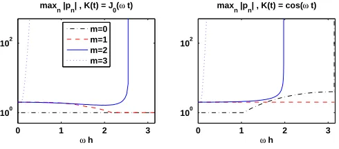
Similar results can be proved for the (more straightforward) oscilla-tory kernelK(t) = cosωt, as summarized below.
0 1 2 3 100
102
ω h max
n |pn| , K(t) = J0(ω t)
0 1 2 3
100 102
ω h max
n |pn| , K(t) = cos(ω t)
[image:27.432.103.348.110.218.2]m=0 m=1 m=2 m=3
Figure 4. Plots of max{|pn|: 0≤n≤2500} againstωh for the B-spline schemes withm= 0 : 3 applied to the highly oscillatory kernels K(t) =J0(ωt) (left plot) andK(t) = cosωt (right plot). (See text for more details.)
• m=1. The scheme is stable at any frequency ω for which ωh∈[0,2π).
• m=2. The scheme is stable at any frequency ω for which ωh∈[0, θ), where θ= 1.9747. . ..
• m=3. There is noO(1) interval of stability for ωh, but the scheme is stable for boundedω.
The stability results for highly oscillatory kernels are illustrated in Figure 4. The plots show maxn|pn| for n= 0 : 2500 for the B-spline
schemes withm= 0 : 3 applied to the kernelsK(t) =J0(ωt) (left plot) andK(t) = cosωt(right plot). Over the rangeω∈[0, π/h] shown, the general stability behavior for these two kernels is similar. In particular, the left plot illustrates the stability whenm= 0,1, while schemem= 2 is stable forωh∈[0, L) withL≈2.55. On the right plot, schemem= 0 is stable except atωh=π, schemem= 1 is stable andm= 2 scheme is stable forωh∈[0, L) withL≈1.97. On both plots them= 3 scheme is clearly unstable whenω=O(1/h).
expansion to show that the same result also holds for smooth K with K(0) = 1 when h is small enough (see, e.g., [6]). Thus, it does not apply to the important case of an oscillatory kernel where the oscilla-tion frequencyω=O(1/h), whose stability was analyzed above for the Bessel function and cosine kernels.
When m= 0, the approximation (3.2) is the same as using piece-wise constant collocation (at the interval endpoints), and this has been fully analyzed (see, e.g.,[6] for details). Here we assume thatm ≥1 (note that this includes the well-known case of piecewise linear approx-imations of (1.2)), and show that convergence is always second order, no matter how high the polynomial degree, because quasi-interpolation by the Schoenberg B-spline operator is at mostO(h2)[14]. This is in marked contrast to discontinuous polynomial collocation or Galerkin approximations of (1.2) which converge at optimal order [6, 7, 8]. However, a simple modification of the B-spline basis near t = 0 can give higher order stable approximations of (1.2), as illustrated when m= 3 in Section 5.
Theapproximation error en(t) forn >0,t≥0 is
(4.11) en(t) =u(tn−t)− n
∑
j=0
vn−jbmj−m(t),
where the coefficientsvj satisfy
(4.12) a(tn) =
n
∑
j=0 qjvn−j
for weightsqj as defined in (4.4). Note thatv0= 0 (becausea(0) = 0), so the sums above can be taken fromj= 0 ton−1, and it then follows from Property P1 that en(t) = 0 for t ≥ tn and each weight can be
written asqj=
∫tn
0 K(t)b
m
j−m(t)dt. Hence, multiplying (4.11) byK(t)
and integrating gives ∫ tn
0
K(t)en(t)dt=
∫ tn
0
K(t)u(tn−t)dt− n∑−1
j=0
qjvn−j = 0,
by (1.2) and (4.12), i.e., en is orthogonal to K on (0, tn). The formal
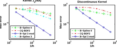
101 102 103 10−4
10−2 100
1/ h
Max error
Kernel cos(4t)
B−Spline 0 B−Spline 1 B−Spline 2 B−Spline 3
101 102 103 10−4
10−2 100
Kernel J 0(4t)
[image:29.432.106.344.111.211.2]1/ h
Figure 5. Convergence results for the approximation of (1.2) for two smooth kernel functions with maximum time T = 10 and a(t) =
t6exp(−50(t−1/2)2). Convergence rates ofO(h2) for splines of degreem≥1
andO(h) form= 0 are clear. Stability results for the highly oscillatory ker-nels cosωt and J0(ωt) where the frequency ω can be O(1/h) are given in subsection 4.2 and Figure 4.
Theorem 4.1. Suppose thatm≥1and the conditions (1.5) and(2.1)
hold ford≥4. Then
(4.13) |en(t)| ≤C h2
for t ∈ [tm, T], for some C independent of n and h. If m = 1, then
(4.13) holds fort∈[0, T].
Remarks.
• Them= 1 case has been fully analyzed[6]and is only included for completeness.
• The restriction to second order convergence for m > 1 is a fundamental aspect of quasi-interpolation by classical B-splines and not an artifact of the proof, and is illustrated in Figure 5 when (2.1) holds withd= 4.
• Equation (4.13) trivially holds for t≥tn (because en(t) = 0),
and so it is enough to prove the result for t ∈ [tm, tn) when
m >1, wheren≤T /h.
Proof. We first expressen(t) in terms of coefficientsεk:=u(tk+(m−1)/2)
u(tn−t) in the definition (4.11) ofen(t) gives
en(t) = n
∑
j=m
εn−jbmj−m(t) + n∑+m
j=n+1
u(tn−tmj−m)b m
j−m(t) +O(h
2),
where we have usedbmj−m(t) = 0 forj < mand j > n+m. It follows from assumptions (1.5) and (2.1) thatu(ch) =O(hd) for any constant c. This implies that the second sum term in the previous equation is
O(hd), and hence yields
en(t) = n
∑
j=m
εn−jbmj−m(t) +O(h
2)
fort∈[tm, tn) withtn ≤T. Because there are at mostm+ 1 nonzero
terms in this sum for anyt, it is sufficient to show that there exists a constantC independent ofhsuch that
(4.14) |εj| ≤Ch2 for allj≤T /h.
To prove (4.14), note that it follows from (4.12) that
n
∑
j=0
qjvn−j=
∫ tn
0
K(t)u(tn−t)dt,
and so
n
∑
j=0 qj
h εn−j=
n
∑
j=0 qj
h u(tn−j+(m−1)/2) (4.15)
− 1
h ∫ tn
0
K(t)u(tn−t)dt:=Rn.
Ifhis sufficiently small, then expandingK(t) and using P4 gives (4.16)
qj
h = {
j+1
m+1 +h K′(0)
(j+1)2(j+2)
2(m+1)(m+2)+O(h
2) forj = 0 :m−1,
K(tj−m) +12h(m+ 1)K′(tj−m) +O(h2) ifj≥m.
It then follows from the quasi-interpolation result (4.3) with p = 3, whenn≥m, that
hRn = n−1 ∑
ℓ=0 3 ∑
k=2