Two-level domain decomposition methods for highly heterogeneous Darcy equations. Connections with multiscale methods

Two-level domain decomposition methods for

highly heterogeneous Darcy equations.

Connections with multiscale methods

Victorita Dolean

_{, Pierre Jolivet}

_{, Frédéric Nataf}

_{*, Nicole Spillane}

_{and Hua Xiang}

1 Laboratoire J.L. Lions, UPMC et CNRS UMR 7598 2 Laboratoire J.A. Dieudonné, Université de Nice

3 School of Mathematics and Statistics, Wuhan University, 430072 Wuhan, P. R. China

e-mail: [email protected] — [email protected] — [email protected]

*Corresponding author

Résumé— —Les écoulements multiphasiques en milieux poreux conduisent à la solution de systèmes d’équations aux dérivées partielles (EDP) à coefficients très hétérogènes. Nous nous concentrons sur les méthodes de décomposition de domaine avec recouvrement de type Schwarz sur calculateurs parallèles et sur les méthodes multi-échelles. Nous présentons un espace grossier [23] qui est robuste, même en présence de telles hétérogénéités. L’approche méthodes de décomposition de domaine à deux niveaux est comparée aux méthodes multi-échelles.

Abstract — — Multiphase, compositional porous media flow models lead to the solution of highly heterogeneous systems of Partial Differential Equations (PDEs). We focus on overlapping Schwarz type methods on parallel computers and on multiscale methods. We present a coarse space [23] that is robust even when there are such heterogeneities. The two-level domain decomposition approach is compared to multiscale methods.

1 INTRODUCTION

Multiphase, compositional porous media flow models, used in reservoir simulations or basin modeling, lead to the so-lution of complex non linear systems of Partial Differential Equations (PDEs). These PDEs are typically discretized us-ing a cell-centered finite volume scheme and a fully implicit Euler integration in time in order to allow for large time steps. After Newton type linearization, one ends up with the solution of a linear system at each Newton iteration which represents up to 90 percents of the total simulation elapsed time. The corresponding pressure block matrix is related to

the discretization of a Darcy equation with high contrasts and anisotropy in the coefficients. We focus on overlapping Schwarz type methods on parallel computers and on multi-scale methods.

that is robust even when there are such heterogeneities. We achieve this by solving local generalized eigenvalue problems which isolate the terms responsible for slow convergence. Building efficient coarse spaces is closely related to multiscale methods which also aim to reduce the computational cost of large scale problems.

An outline of the paper is as follows. Section 2 consists in an introduction to one level Schwarz methods. Material is basic but the presentation is quite new. In § 3, we present a recent spectral coarse space which adapts automatically to the heterogeneities of the problem. In § 4 we present results of large scale computations. In § 5, it is compared to multiscale methods. In section 6, we conclude and present prospects on adaptation of the spectral coarse space to finite volume discretizations.

2 SCHWARZ METHODS

We start with the original Schwarz algorithm [27] at the continuous (i.e. partial differential equations) level whose parallel version is named Jacobi-Schwarz method (JSM). We introduce two variants that are at the origin of the pop-ular additive Schwarz method (ASM) and restricted addi-tive Schwarz (RAS [4]) algorithms. The first one has been the subject of hundreds of papers (see [29] and references therein). The second one is the default parallel solver of the parallel package software PETSc [2]. This presenta-tion shows in a unified setting the connecpresenta-tions between these three algorithms.

2.1 Three Schwarz Algorithms at the continuous

level

Hermann Schwarz was a German analyst of the 19th cen-tury. He was interested in proving existence and uniqueness of the Poisson problem. At his time, there were no Sobolev spaces nor Lax-Milgram theorem. The only available tool was the Fourier transform, limited by its very nature to sim-ple geometries. In order to consider more general situations, H. Schwarz devised an algorithm based on solving itera-tively Poisson problem set on a union of simple geometries. Let the domainΩbe the union of a disk and a rectangle, see Figure 1 and consider the Poisson problem:

Findu:Ω→_Rsuch that:

−∆u= f inΩ u=0 on∂Ω.

(1)

The Schwarz algorithm is an iterative method based on solving alternatively subproblems in domains Ω1 andΩ2.

Ω

₁

Ω

2

Figure 1

A complex domainΩmade from the union of two simple ge-ometries

It updates (un

1,u

n

2)→(u

n+1 1 ,u

n+1 2 ) by:

−∆(un₁+1)= f inΩ1 un₁+1=0 on∂Ω1∩∂Ω un₁+1=u₂n on∂Ω1∩Ω2.

then,

−∆(un₂+1)=f inΩ2 un₂+1=0 on∂Ω2∩∂Ω u₂n+1=u₁n+1 on∂Ω2∩Ω1.

(2) H. Schwarz proved the convergence of the algorithm and thus the well-posedness of the Poisson problem in complex geometries.

With the advent of digital computers, this method also ac-quired a practical interest as an iterative linear solver. Sub-sequently, parallel computers became available and a small modification of the algorithm makes it suited to these archi-tectures. It is sufficient to solve concurrently in all subdo-mains,i=1,2:

−∆(un+1

i )= f in Ωi

un+1

i =0 on ∂Ωi∩∂Ω

un+1

i =u

n

3−i on ∂Ωi∩Ω3−i.

(3)

It is easy to see that if the algorithm converges, the solutions u∞

i ,i = 1,2 in the intersection of the subdomains take the

same values. Indeed, in the overlapΩ12 := Ω1 ∩Ω2, let e∞_:=u∞

1 −u

∞

2. By the last line of (3), we know thate

∞₌₀

on∂Ω12. By linearity of the equation, we also have thate∞

is harmonic. Thus,e∞_{solves the homogeneous well posed}

BVP:

−∆(e∞)=0 in Ω12 e∞=0 on ∂Ω12

and thuse∞_{=0 .}

Algorithms (2) and (3) act on the local functions (ui)i=1,2.

In order to write algorithms that act on global functions in H1_{(Ω), the space in which problem (1) is naturally posed,} we need extension operators, Eiso that for a functionwi :

Ωi 7→ R,Ei(wi) : Ω 7→ Ris the extension of wi by zero

Ωi7→R,χi≥0 andχi(x)=0 forx∈∂Ωiand such that:

w= 2

X

i=1

Ei(χiw|_Ωi) (4)

for any functionw :Ω 7→ _R. This definition of a partition of unity is closer to the computer implementation than the classical definition of a partition of unity functions.

There are two ways to write related algorithms that act on functionsun _{∈ H}1_{(Ω). The first possibility is : Letu}n _be

an approximation to the solution to the Poisson problem (1), un+1_{is computed by solving first local subproblems:}

−∆(un+1

i )= f in Ωi

un+1

i =0 on ∂Ωi∩∂Ω

un+1

i =u

n _{on ∂Ω}

i∩Ω3−i.

(5)

and then gluing them together using the partition of unity functions:

un+1 := 2

X

i₌1

Ei(χiuni+1). (6)

A second possibility consists in replacing the above formula by a simpler formula not based on the partition of unity:

un+1:= 2

X

i=1

Ei(uni+1). (7)

Starting from the original Schwarz algorithm (2) that is se-quential, we have thus three continuous algorithms that are essentially parallel:

• Algorithm (3) Jacobi Schwarz Method (JSM)

• Algorithm (5)-(6) Restricted Additive Schwarz (RAS)

• Algorithm (5)-(7) Additive Schwarz Method (ASM) These algorithms although closely related are different in nature. The JSM method acts on a pair of local functions (un

1u

n

2) whereas RAS and ASM act on a global functionu

n_.

Note that in the overlapping region, algorithms RAS and ASM update the solution in a different way. Algorithm ASM seems rather bizarre since it does not converge to the exact solution in the intersectionΩ1∩Ω2. But its algebraic form given by (10) when used a preconditioner as explained in the sequel has the advantage to be symmetric positive defi-nite (SPD). On the contrary the algebraic counterpart to RAS given by (9) is unsymmetric.

2.2 Schwarz Algorithms at the algebraic level

So far, we have given a continuous presentation of domain decomposition methods. Actually, these methods are used in their algebraic form to solve linear systems arising from the discretization of partial differential equations. We now give the matrix counterpart of these algorithms.

For this, we first give a kind of dictionary to go from the continuous level to the discrete one:

– the counterparts of a domainΩand of an overlapping de-compositionΩ =∪N_i=1Ωiare a set of degrees of freedom

(d.o.f.)Nand a decomposition in subsetsN =∪N_i=1Ni.

– a functionu:Ω→_Rcorresponds a vectorU∈_R#N_.

– the restriction of a functionu : Ω → _Rto a subdomain

Ωi, 1≤i≤Nis analog to the restrictionRiUof a vector

U∈_R#N_{to subsetN}

i. MatrixRiis a Boolean rectangular

of size #N_i×#N.

– similarly, Ei(ui) the extension by zero of a functionui :

Ωi→Rto a functionΩ→Rcorresponds at the algebraic

level toRT

i UiwhereR T

i is the transpose of matrixRiand

Ui∈R#Ni_{is a local vector.}

– the counterparts of partition of unity functionsχi, 1≤i≤ Nare diagonal matrices with positive entries, of size #Ni×

#Nis. t.Id=PNi=1R

T

i DiRi.

– After discretization, solving Poisson problem (1) amounts to solving a SPD linear system

A U =F. (8)

– Solving a local subproblem in a subdomainΩisuch as in

equations (3) or (5) corresponds at the algebraic level to solving linear systems of the formRiA RTi U

n+1

i =F

n i.

We now define, at the algebraic level, the RAS and ASM algorithms and not JSM since it is seldom used and is more complex to define. As for the counterpart of the RAS algo-rithm (5)-(6), we give the following definition

M−_RAS1 :=

N X

i=1

RT_i Di(RiA RTi)

−1_R

i (9)

so that the iterative RAS algorithm reads:

Un+1=Un+M_RAS−1 rn

wherern:=F−A Un.

As for the counterpart of the ASM algorithm (5)-(7), we give the following definition

M−_{AS M}1 :=

N X

i=1

RT_i (RiA RTi)

−1_R

i (10)

so that the iterative ASM algorithm reads:

Un+1=Un+M−_{AS M}1 rn.

preconditioned by the symmetric preconditioner MAS M or

by a GMRES algorithm preconditioned by the unsymmetric preconditioner MRAS. In both cases, the convergence

properties are related to the spectral properties of the pre-conditioned operatorM−_{AS M}1 _orRASA. Therestricted additive Schwarzmethod (RAS, see[3]) is the default parallel solver in the PETSc package. For the additive Schwarz method (ASM) many theoretical results have been derived, see [29] and references therein.

3 ADAPTIVE SPECTRAL COARSE SPACE

The domain decomposition methods presented so far were written for a two subdomain decomposition. Their extension to an arbitrary numberNof subdomains (Ωi)1≤i≤N is only a

matter of notation. It is sufficient in definitions of the previ-ous section to sum over all subdomains fromi=1 toi=N. But, when the number of subdomains is large, plateaus ap-pear in the convergence of Schwarz domain decomposition methods. This is the case even for a regular problem such as the Poisson problem (1). The problem comes from the fact the preconditioner lacks of a global mechanism for ex-change of information. Preconditioners RAS and ASM de-fined in the previous sections are called one-level methods. Data are exchanged only from one subdomain to its direct neighbors. But the solution in each subdomain depends on the right handside in all subdomains. Let us callNdthe

num-ber of subdomains in one direction. Then, for instance, the leftmost domain of Figure 3 needs at leastNditerations

be-fore knowing something about the value of the right hand-side fin the rightmost subdomain. The length of the plateau is thus typically related to the number of subdomains in one direction and therefore to the notion ofscalabilitymet in the context of high performance computing.

In order to achieve scalability of the domain decomposi-tion (DD) method, we introduce two-level domain decom-position methods via a coarse space correction. The precise motivation and linear algebra setting are given in § 3.1 for a problem with smooth coefficients. A new approach § 3.2 in-troduced in [22, 23] is necessary to achieve scalability for ar-bitrary highly heterogeneous coefficients. A condition num-ber estimate theorem supports the approach. The method is tested in § 3.4 on difficult heterogeneous test cases including channelized medium. In practice, the coarse space seems to be optimal, see Table 10 in § 3.4.1.

3.1 Need for a two-level method

When the number of subdomains is large, plateaus appear in the convergence of Schwarz domain decomposition methods. The remedy will consist in the introduction of a

-7 -6 -5 -4 -3 -2 -1 0

0 10 20 30 40 50 60 70 80

Log_10 (Error)

Number of iterations (GCR) M2

2x2

2x2 M2

4x4 M2 8x8

4x4 8x8

Figure 2

Japhet, Nataf and Roux [19]

two-level preconditioner via a coarse space correction.

The problem and its cure are well illustrated in Figure 4 for a domain decomposition into 64 strips. The one level method has a long plateau in the convergence whereas with a coarse space correction convergence is quite fast. For in-stance, in Figure 2 we consider a 2D problem decomposed into 2×2, 4×4 and 8×8 subdomains. For each domain decomposition, we have two curves: one with a one-level method and the second with a coarse grid correction which is denoted by M2. We see that for the one-level curves, the plateau has a size proportional to the number of subdomains in one direction. In two-level methods, a small problem of size typically the number of subdomains couples all subdo-mains at each iteration. It is through this mechanism that scalability can be achieved.

Figure 3

Decomposition into many subdomains

From a condition number point of view, stagnation corresponds to a few very low eigenvalues in the spectrum of the preconditioned problem. Using preconditioners MAS Mor MRAS, we can remove the influence of very large

eigenvalues of the coefficient matrix, which correspond to high frequency modes. Indeed, it has been proved that for a SPD matrix, the largest eigenvalue of the preconditioned system by MAS M is bounded by the number of colors

colors for adjacent subdomains, see [29] or [26] for in-stance. But the small eigenvalues still exist and hamper the convergence. These small eigenvalues correspond to low frequency modes and represent certain global information. We need a suitable coarse grid space to efficiently deal with them.

A classical remedy consists in the introduction of a coarse grid or coarse space correction that couples all subdomains at each iteration of the iterative method. This is closely re-lated to deflation technique classical in linear algebra, see Nabben and Vuik’s paper [21] and references therein. Sup-pose we have identified the modes corresponding to the slow convergence of the iterative method used to solve the linear system:

Ax=b

with a preconditioner M, in our case a domain decomposi-tion method. That is, we have some a priori knowledge on the small eigenvalues of the preconditioned system M−1A. For a Poisson problem, these slow modes correspond to constant functions that are in the null space (kernel) of the Laplace operators. For a homogeneous elasticity problem, they correspond to the rigid body motions. Let us callZthe rectangular matrix whose columns correspond to these slow modes. There are algebraic ways to incorporate these in-formations to accelerate the domain decomposition method. We give here the presentation that is classical in domain de-composition methods. In the case whereAis SPD, the start-ing point is to consider the minimization problem

min

β kA(y+Zβ)−bkA−1.

It corresponds to finding the best correction to an approxi-mate solutionyby a vectorZβin the vector space spanned by thenccolumns ofZ. This problem is equivalent to

min

β∈Rnc2(Ay−b,Zβ)2+(AZβ,AZβ)2

and whose solution is:

β=(ZTAZ)−1ZT(b−Ay).

Thus, the correction term is:

Zβ=Z(ZTAZ)−1ZT(b−Ay).

LetR0 :=ZT andr =b−Aybe the residual associated to the approximate solutiony, the best correction that belongs to the vector space spanned by the columns ofZreads:

RT₀ (R0ART₀)−1R0r.

When using such an approach with an additive Schwarz method (ASM), it is natural to introduce an additive cor-rection to the additive Schwarz method:

M−_{AS M}1 _,2:=RT₀(R0ART₀)−1R0+

N X

i=1

RT_i(RiARTi)

−1

Ri (11)

where theRi’s (1 ≤ i ≤ N) are the restriction operators to

the overlapping subdomains. The structure of the two level preconditioner M−_{AS M}1 _,2 is thus the same than in the one level method. Compared to the one level Schwarz method where only local subproblems have to be solved in parallel, the two-level method adds the solution of a linear system in a sequential way with the matrixR0ART₀. This problem couples all subdomains at each iteration. But this matrix is a smallO(N×N) square matrix and the extra cost is negligible compared to the gain. Indeed, in Table 1 we display the iteration counts for a decomposition of the domain in an increasing number of subdomains. In figure 4, we see that without a coarse grid correction, the convergence curve of the one level Schwarz method has a very long plateau that can be bypassed by a two-level method.

N subdomains Schwarz With coarse grid

4 18 25

8 37 22

16 54 24

32 84 25

64 144 25

TABLE 1

Iteration counts for a Poisson problem on a domain decomposed into strips. The number of unknowns is proportional to the number of

subdomains (weak scalability).

0 50 100 150

10−8

10−6

10−4

10−2

100

102

104

X: 25

Y: 1.658e−08

SCHWARZ

additive Schwarz with coarse gird acceleration

Figure 4

Convergence curves with and without a coarse space correction for a decomposition into 64 strips

sub-domains and so that the constant function1belongs to the vector space spanned byZ. Recall that we have a partition of unity in the following sense: letDi, 1≤i≤N, be matrices

Di:Rdim(Ni)7−→Rdim(Ni) (12)

so that we have:

N X

i=1

RT_iDiRi=Id.

We defineZsuch that thei-th column ofZis:

Zi:=RTi DiRi1for 1≤i≤N (13)

where1is the vector full of ones. The structure ofZis thus the following:

ZNico =                    

D1R11 0 · · · 0

..

. D2R21 · · · 0

..

. ... · · · ... 0 0 · · · DNRN1

                    . (14)

The results of Figures 4 and Table 1 were obtained using this method.

0 50 100 150 200 250 300 350

10−6 10−4 10−2 100 102 104 106 AS P

ADEF2: AS + Z Nico P

ADEF2: AS + Z D2N RAS P

ADEF2: RAS + Z Nico P

ADEF2: RAS + Z D2N

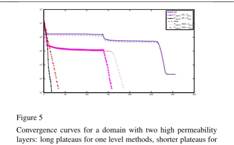
Figure 5

Convergence curves for a domain with two high permeability layers: long plateaus for one level methods, shorter plateaus for Nicolaides coarse spaces and no plateau for DtN coarse space

For problems of the type−div(α∇u)= f with smooth co-efficientsα, this coarse space gives good results. But for highly heterogeneous coefficients, there is still a plateau in the convergence of the solver. The results in Figure 5 cor-respond to a domain which has two layers with high values ofα. The computational domain has a stripwise decompo-sition into 64 subdomains. Two Schwarz methods are tested with either no coarse space correction, a Nicolaides coarse space or a spectral coarse space defined in § 3.2 so a to-tal of six curves. The curves with very long plateaus are one level Schwarz methods. The curvesZNico(pink curves)

correspond to two level Schwarz methods with a Nicolaides coarse space, equation (13). The plateau in the conver-gence is not as large but still exists. With the spectral coarse space of the next section, we automatically select two modes per subdomain and get the convergence curvesZD2N (black

curves).

3.2 Spectral coarse space for highly heterogeneous

problems

We now propose a construction of the coarse space that will be suitable for parallel implementation and efficient for ac-celerating the convergence for problems with highly hetero-geneous coefficients of the type

−div(α∇u) = f inΩ,

B(u) = 0 on∂Ω (15)

withαa positive function. We still chooseZsuch that it has the form Z=                    

W1 0 · · · 0

..

. W2 · · · 0

..

. ... · · · ... 0 0 · · · WN

                    , (16)

where N is the number of overlapping subdomains. But Wi _{is now a rectangular matrix whose columns are based}

on the harmonic extensions of the eigenvectors correspond-ing to small eigenvalues of the Dirichlet-to-Neumann (DtN) map in each subdomainΩi. Remark that the sparsity of the

coarse operatorE = ZT_{AZ is a result of the sparsity ofZ.}

The nonzero components ofEcorrespond to adjacent sub-domains.

More precisely, let us consider first at the continuous level the Dirichlet to Neumann map DtN_Ωi. Let u : Γi 7→ R,

(Γi:=∂Ωi\∂Ω)

DtN_Ωi(u)=α∂v

∂ni _Γ i ,

wherevsatisfies

      

L(v) :=−div(α∇)v=0, in Ωi,

v=u, onΓi, (17)

andΓi is the interface boundary. If the subdomain is not a

floating one (i.e. ∂Ωi∩∂Ω ,∅), we use on the part of the

global boundary, the boundary condition from the original problemB(u) = 0. To construct the coarse grid subspace, we use the low frequency modes associated with the DtN operator:

DtN_Ωi(u)=λαu (18)

with

λ <1/diam(Ωi) (19)

wherediam(Ωi) is the diameter of subdomainΩi. The

ra-tionale for this choice is that the condition number estimate of Theorem 3.2 is then similar to the one of Theorem 3.1 for the Poisson problem. Note the termαin the generalized eigenvalue problem (18).

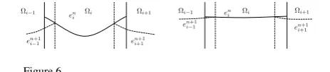
We first motivate our choice of a coarse space based on DtN map. We write the original Schwarz method at the con-tinuous level, where the domainΩis decomposed in a one-way partitioning, see Figure 6. The error en

Ωi Ωi+1

Ωi−1 _en

i

en+1

i−1 en+1i+1

Ωi Ωi+1

Ωi−1 en

i

en+1

i−1 en+1

i+1

Figure 6

Fast or slow convergence of the Schwarz algorithm.

current iterate at stepnof the algorithm and the solutionu|_Ωi

(en

i :=u

n

i −u|Ωi) in subdomainΩiat stepnof the algorithm

satisfies:

L(en+1

i )=0 in Ωi,

en_i+1=en_j on ¯Ωi∩∂Ωj.

On the 1D example sketched in Figure 6, we see that the rate of convergence of the algorithm is related to the decay of the harmonic functionsen_i in the vicinity of∂Ωi viathe

subdomain boundary condition. Indeed, a small value for this boundary condition leads to a smaller error in the entire subdomain thanks to the maximum principle.

Moreover a fast decay for this value corresponds to a large eigenvalue of the DtN map whereas a slow decay corre-sponds to small eigenvalues of this map because the DtN operator is related to the normal derivative at the interface and the overlap is thin. Thus the small eigenvalues of the DtN map are responsible for the slow convergence of the al-gorithm and it is natural to incorporate them in the coarse grid space.

We now explain why we only keep eigenvectors with eigenvalues smaller than 1/diam(Ωi) in the coarse space.

We start with the constant coefficient caseα = 1. In this case, the smallest eigenvalue of the DtN map is zero and it corresponds to the constant function 1. For a shape regular subdomain, the first positive eigenvalue is of order 1/diam(Ωi), see [12]. Keeping only the constant function

1 in the coarse space leads to good numerical convergence, see figure 4. In the case of high contrasts in the coefficient

α, the smallest eigenvalue of the DtN map is still zero. But due to the variation of the coefficients we may possibly have positive eigenvalues smaller than 1/diam(Ωi). In

order to have a convergence behavior similar to the one of the constant coefficient case, it is natural to keep all eigenvectors with eigenvalues smaller than 1/diam(Ωi).

To obtain the discrete form of the DtN map, we consider the variational form of (17). Let’s define the bilinear form ai:H1(Ωi)×H1(Ωi)→R,

ai(w,v) := Z

Ωi

α∇w· ∇v.

With a finite element basis{φ_k}, the coefficient matrix of a Neumann boundary value problem in domainΩiis

A(_kli)=

Z

Ωi

α∇φ_k· ∇φ_l.

LetI(resp.Γi) be the set of indices corresponding to the

in-terior (resp. boundary) degrees of freedom andn_Γi :=#(Γi)

the number of interface degrees of freedom. Note that for the whole domainΩ, the coefficient matrix is given by

Akl= Z

Ωα

∇φk· ∇φl.

With block notations, we have

A(_IIi) =AII, A(_Γi)

iI =AΓiI and A

(i)

IΓi =AIΓi.

But the matrixA(_Γi)

iΓi refers to the matrix prior to assembly

with the neighboring subdomains and thus cannot be simply extracted from the coefficient matrixA. In problem (17), we use Dirichlet boundary conditions. LetU ∈ _RnΓi and

u := P

k∈ΓiUkφk. Let v :=

P

k∈IVkφk+Pl∈ΓiVlφl be the

finite element approximation of the solution of (17). Let VI =(Vk)k∈I, we have with obvious notations:

AIIVI+AIΓiU=0. (20)

A variational definition of the flux reads

Z

Γi

α∂v

∂nφk=

Z

Ωi

α∇v· ∇φ_k

for allφk,k∈Γi. So the variational formulation of the

eigen-value problem (18) reads

Z

Ωi

α∇v· ∇φ_k =λ

Z

Γi

tr(α)vφk (21)

for allφk,k∈Γiand wheretr(α) is the restriction ofαΩito

Γi. LetMα,Γibe the weighted mass matrix

(Mα,Γi)kl:=

Z

Γi

tr(α)φkφl, ∀k,l∈Γi.

The compact form of equation (21) is

A(_Γi)

iΓiU+AΓiIVI =λMα,ΓiU.

With (20), the discrete form of (18) is a generalized eigen-value problem

(A(_Γi)

iΓi−AΓiIA

−1

IIAIΓi)U=λMα,ΓiU. (22)

Let (Uλ, λ) be an eigenpair, we need its harmonic extension

to the degrees of freedom of domainΩi, that is the vector:

"

−A−1

IIAIΓiUλ

Uλ

# .

Actually, there is more practical way todirectly compute these eigenpairs. For subdomainΩi, let

v:=

"

VI

V_Γi

#

,A(i) :=

"_A

II AI_Γi

A_ΓiI A(_Γi)_iΓi #

we compute the lowest eigenvalues of the sparse generalized eigenvalue problem:

A(i)vdtn=λ "

0 0

0 Mα,Γi

#

vdtn. (23)

This can be done using standard linear algebra library such as ARPACK.

The step by step procedure on how to construct the rectangular matrices Wi _{in the coarse space matrixZ, see}

(16), is summed up in Algorithm 1. We call this procedure

Algorithm 1Construction of the spectral coarse space In parallel for all subdomains 1≤i≤N,

1. Compute eigenpairs of (23) (Vi

1, λ

i

1),(V

i

2, λ

i

2), . . . ,(V

i

mi, λ

i

mi) such that

λi

1≤. . .≤λ

i

mi <1/diam(Ωi)≤λ

i

m_i+1≤. . .

2. LetZde defined as in (16) with for each 1≤i≤N,Wi the rectangular matrix withmicolumns defined by

Wi=[DiV1i|. . .|DiVmii].

3. NoteR0:=ZT_{and compute the coarse matrixE:}

E:=R0A RT₀.

4. The two-level preconditioner is given by eq. (11):

M−_{AS M}1 _,2:=RT₀E−1R0+

N X

i=1

RT_i(RiARTi)

−1 Ri

the ZD2N method. We also useZD2N to denote the coarse

space constructed by this method. Its construction is fully parallel. Similarly we callZNico the method of Nicolaides

or the corresponding coarse space. Let us remark that when the subdomain does not touch the boundary ofΩ, the lowest eigenvalue of the DtN map is zero and the corresponding eigenvector is a constant vector. Thus, ZNico and ZD2N

coincide. As we shall see in the next section, when a subdomain has several jumps of the coefficient, takingZNico

is not efficient and it is necessary to takeZD2N with more

than one mode per subdomain.

This construction has been analyzed in [7]. We first recall a classical result. LetZbe a “Nicolaides type” coarse space

Z:=(RT_i DiRi1)1≤i≤N.

We have, see [29]:

Theorem 3.1 Let MAS M,2be the two-level additive Schwarz method with the “Nicolaides” coarse space , we have for

α=1the following condition number estimate:

κ(M_{AS M}−1 _,2A)≤C(1+H

δ)

whereδis the size of the overlap between the subdomains and H the subdomain size and C does not depend on the number of subdomains.

But, forαdiscontinuous,C would depend on the jumps of

α.

LetZ be the coarse space built via Algorithm 1, we prove under technical assumptions onα

Theorem 3.2 Under the monotonicity ofαin the overlap-ping regions, we have the following condition number esti-mate:

κ(M−_{AS M}1 _,2A)≤C(1+max

1≤i≤N

1

δiλi_mi+1

)

whereδi is the size of the overlap of domainΩi and C is

independent of the jumps ofαand of the number of subdo-mains.

Note that ifα = 1 and we take only one mode per subdo-main (mi = 1), we have for a regular interfaceλi2 ' 1/Hi

(see [12]) and we recover the “classical” estimate. Now in the general case, if the number of modes associated to subdomainΩimiis chosen so that,λimi+1 ≥1/Hi, the

con-vergence rate will be analogous to the constant coefficient case.

3.3 Comparison with a volumic spectral coarse

space

The DtN spectral coarse space makes use of eigenvectors of the local Dirichlet to Neumann maps. There is thus a clear relationship with recent works by Galvis and Efendiev [9, 10, 13–15] where the coarse space is based on eigenvalues of thevolumicoperator

−div(α∇ui)=λ αuiinΩi. (24)

The drawback of their approach is that the coarse space is too large. This is easy to see in 1D. In Figure 7, we repre-sent the functionαin a subdomainΩi. We have many

Ω

Ω

Ω

Figure 7

1D example with many high heterogeneities islands

volumic eigenvalues of eq. (24) are smaller than 3.8e−3 and the others are larger than 150. Numerical tests show that in this case only four eigenvalues are enough for having an ef-ficient coarse space. In the papers by Galvis and Efendiev, they noted this fact and they have a complex procedure to get rid of the useless eigenvectors. In our case, the method adapts automatically to the permeability field. In Figure 9 we show typical DtN and volumic eigenvectors.

IsoValue

-42104.2

21053.6

63158.8

105264

147369

189474

231580

273685

315790

357895 400000

442106

484211

526316

568421

610527

652632 694737

736842

842105

Figure 8

2D example with many high heterogeneities islands

3.4 First Numerical tests

We solve the model problem (15) on the domainΩ =[0,1]2 using standard continuous, piecewise linear (P1) finite ele-ments. The diffusionαis a function ofx. The boundary con-dition isu=0 on the left side boundary and∂u

∂n =0 on the

re-mainder. The corresponding discretizations and data struc-tures were obtained by using the software FreeFem++[17] in connection with the METIS partitioner [20]. We will test the standard additive Schwarz (ASM) and the restricted additive Schwarz (RAS) preconditioners with and without coarse space, in particular comparing the new coarse space based on harmonic extensions of eigenvectors of the lo-cal DtN operators with the standard coarse space that is

Figure 9

Eigenvectors for: DtN map (left) and the volumic operator (right) (Freefem++plots)

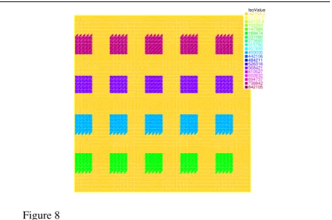
the piecewise constant space of Nicolaides [24]. In the ta-bles and figures, +Nico means the use of the Nicolaides coarse space (14) and+DtN the use of the spectral coarse space defined in Algorithm 3.2. We test the method on (fairly irregular) overlapping partitions intoN subdomains. These overlapping partitions are built by adding layers to non-overlapping ones obtained, e.g., via graph partitioner METIS (see Figure 13).

In Table 2, we test robustness w.r.t. the heterogeneities. The domainΩcontains layers with jumps in the coefficients ranging from 1 to 106_{. We have 32 subdomains. The} iter-ation counts depend weakly on the size of the jump in the coefficients. In Figure 10, we show the permeability field,

Jumps in coeff 1 10 102 103 104 105 106

Iteration counts 15 24 10 10 10 11 11

TABLE 2

Iteration counts vs. jumps in the coefficients

domain decomposition (regular or METIS) into 16 subdo-mains and the solution corresponding to convergence curves of Figures 11 and 12. In Table 3, we show how many eigen-values were selected in the coarse space. In Table 4, we vary the domain decomposition for the same permeability field.

We now present a selection of difficult test cases in a more systematic way, with so called inclusions and channels.

We solve two test cases with known difficulties. The dif-fusion coefficientαis highly heterogeneous and takes val-ues between 1 and approximately 2×106_{and contains both} high-permeability inclusions and channels. First of all we will analyze the performance of the method by increasing the number of channels and then by increasing the number of inclusions.

IsoValue -78946.3 39474.7 118422

197369 276317

355264 434211 513159 592106 671053 750001 828948 907895 986842 1.06579e+06 1.14474e+06 1.22368e+06 1.30263e+06 1.38158e+06

1.57895e+06

IsoValue -0.0079688 0.0039844 0.0119532

0.019922 0.0278908

0.0358596 0.0438284 0.0517972 0.059766 0.0677348 0.0757036 0.0836724 0.0916412 0.09961 0.107579 0.115548 0.123516 0.131485 0.139454

0.159376

Figure 10

Channels and inclusions: 1≤α≤1.5 106_{. Top left:} permeabil-ity field, top right: the solution, bottom left: regular partition and permeability field, bottom right: Metis partition and permeabil-ity field

0 20 40 60 80 100 120 140 160 180

10−9

10−8

10−7

10−6

10−5

10−4

10−3

10−2

10−1

100

101

Iteration count

Error

RAS PBNN : RAS + ZNico

P

BNN : RAS + ZD2N

Figure 11

RAS convergence for channels and inclusions – Regular parti-tioning

0 50 100 150

10−8

10−7 10−6

10−5

10−4

10−3 10−2

10−1

100

101

Iteration count

Error

RAS PBNN : RAS + ZNico

P

BNN : RAS + ZD2N

Figure 12

RAS convergence for channels and inclusions – Regular decom-position – Metis partitioning

subdomaini nsmeig(i) total number of eigenval.(i)

1 3 155

2 1 109

3 5 175

10 4 174

11 2 71

12 2 128

13 3 166

14 3 127

15 3 188

16 3 106

TABLE 3

Number of small eigenvalues (nsmeig(i)) satisfying criterion (19) for subdomaini– Metis 4 by 4 decomposition

ASM +Nico +DtN RAS +Nico +DtN

2×2 103 110 22 70 70 14

2×2 Metis 76 76 22 57 57 18

4×4 603 722 26 169 165 15

4×4 Metis 483 425 36 148 142 23

8×8 461 141 34 205 95 21

8×8 Metis 600 542 31 240 196 19

TABLE 4

Convergence results for the test case of Figure 10

Figure 13

. We use the ASM preconditioner within conjugate gradi-ents (CG) and the RAS preconditioner within GMRES, and in each case we stop the iteration process, when the relative residual is smaller than 10−6.

IsoValue -47367.4 23685.2 71053.6

118422 165790

213159 260527 307895 355264 402632 450001 497369 544737 592106 639474 686842 734211 781579 828947

947368

IsoValue -99998.9 50001 150001

250001 350001

450001 550001 650001 750001 850001 950000 1.05e+06 1.15e+06 1.25e+06 1.35e+06 1.45e+06 1.55e+06 1.65e+06 1.75e+06

2e+06

IsoValue -121052 60527.3 181580

302632 423685

544738 665790 786843 907895 1.02895e+06 1.15e+06 1.27105e+06 1.39211e+06 1.51316e+06 1.63421e+06 1.75526e+06 1.87632e+06 1.99737e+06 2.11842e+06

2.42105e+06

IsoValue -142104 71053.6 213159

355264 497369

639474 781580 923685 1.06579e+06 1.2079e+06 1.35e+06 1.49211e+06 1.63421e+06 1.77632e+06 1.91842e+06 2.06053e+06 2.20263e+06 2.34474e+06 2.48684e+06

2.84211e+06

Figure 14

Test Problem 1: Successively adding channels.

ASM +Nico. +DtN RAS +Nico. +DtN

0 ch. 529 1000 57 243 245 41

1 ch. 619 520 64 227 228 46

2 ch. >1000 516 68 226 226 47

3 ch. 585 697 76 212 213 44

TABLE 5

Number of iterations for Test Problem 1 (additive coarse grid correction).

We start with only inclusions and add the channels one by one as shown in Figure 14 (Test Problem 1). When there are no channels,αvaries between 1 and 106, as indicated by the colors in Figure 14. With all three channels present,

αvaries between 1 and 2.8×106. The corresponding con-vergence results are given in Table 5. Our algorithm per-forms significantly better. The piecewise constant coarse space has virtually no effect on the performance of either ASM or RAS, leading to iteration numbers that differ little from the results without any coarse grid in all four cases. Our new coarse space, on the other hand, is fully robust to the coefficient variation and to the addition of channels, and it leads to a gain of at least a factor 8 compared to the one-level method in all cases. The situation is similar, if we use deflation-based coarse grid correction [21] with the same coarse spaces (see Table 6). However, the absolute numbers of iterations are reduced almost by a factor 2 in this case. Our theory applies equally to this case (see e.g. [16] for de-tails), but we will not include any further numerical results with deflation-based coarse grid correction.

Table 7 gives some information on the size of the coarse

ASM +Nico. +DtN RAS +Nico. +DtN

0 ch. 529 656 39 243 231 25

1 ch. 619 538 41 227 215 28

2 ch. >1000 808 47 226 211 27

3 ch. 585 641 47 212 199 28

TABLE 6

Number of iterations for Test Problem 1 (deflation-based coarse grid correction).

space that we build with our automatic selection strategy: for each number of channels we give minjmjand maxjmj,

as well as the global coarse space sizenH =Pjmjand the

average number of modes included per subdomain nH/N. For comparison, we also include information on the total numbern_Γj of eigenmodes of the discrete DtN operator on

each subdomain. We note that adding channels does not have a big influence on the size of the coarse space; we only need three additional eigenvectors in the case of three chan-nels compared to the case of no chanchan-nels.

Over 16 # eigenval. # local coarse space modes subdom. onΓj 0 ch. 1 ch. 2 ch. 3 ch.

Min. 70 1 1 1 1

Max. 191 4 4 4 4

Average 138.8 2.75 2.88 2.94 2.94

Sum 2220 44 46 47 47

TABLE 7

Size of the coarse space for Test Problem 1 with various number of channels.

Then, using the same domain and the same partition we successively add inclusions without any channels present as shown in Figure 15 (Test Problem 2). The results are in Table 8. Again, the piecewise constant coarse space is not working at all for this test problem. The DtN-based coarse space is almost completely robust to an increase in the num-ber of inclusions and requires again significantly less itera-tions than the one-level method in all cases. Note that the subdomain partition (cf. Figure 13) is not aligned with the inclusions at all (cf. Figure 15). In Table 9 we see that also in this test problem, the coarse space size grows only very slowly with the number of inclusions and even in the hardest casenHis only 53 (cf. the dimensionnofVh,0, and thus of Ais 25600).

3.4.1 Practical optimality of the spectral coarse space

au-IsoValue -15788.4 7895.71 23685.1

39474.6 55264

71053.4 86842.8 102632 118422 134211 150000 165790 181579 197369 213158 228948 244737 260526 276316

315789

IsoValue -26314.7 13158.9 39474.6

65790.3 92106.1

118422 144738 171053 197369 223685 250000 276316 302632 328948 355263 381579 407895 434211 460526

526316

IsoValue -47367.4 23685.2 71053.6

118422 165790

213159 260527 307895 355264 402632 450001 497369 544737 592106 639474 686842 734211 781579 828947

947368

IsoValue -57893.7 28948.3 86843

144738 202632

260527 318422 376316 434211 492106 550000 607895 665790 723685 781579 839474 897369 955263 1.01316e+06

1.15789e+06

Figure 15

Test Problem 2: Successively adding inclusions.

# incl. ASM +Nico +DtN RAS +Nico +DtN

2×2 108 80 51 100 81 41

3×3 194 342 58 154 153 46

5×5 529 no cv. 57 243 245 41

6×6 835 823 71 266 267 51

TABLE 8

Number of iterations for Test Problem 2 (additive coarse grid correction) vs. number of inclusions.

OverN=16 # eigen. # local coarse space modes subdomains onΓj 0 ch. 1 ch. 2 ch. 3 ch.

Minimum 70 1 1 1 1

Maximum 191 3 3 4 5

Average 138.8 1.6 2.1 2.8 3.3

Sum 2220 26 33 44 53

TABLE 9

Size of the coarse space for Test Problem 2.

tomatic algorithm is indeed optimal in some sense. For Test Problem 1 with one channel (see Figure 14), we first reduce the number of coarse basis functions per subdomain by one, this has a huge influence on the iteration count. Then we add one basis function per subdomain and notice that this has much less effect. This suggests that the selection process we have designed is indeed the best compromise between en-riching the coarse grid and solving a reasonably sized coarse problem.

ASM RAS

No coarse space 619 227

Piecewise constant coarse space 520 228 DtN with max{mj−1,1}functions 446 177

DtN withmjfunctions 64 46

DtN withmj+1 functions 37 32

TABLE 10

Iteration numbers when reducing or increasing the numbermjof coarse basis functions per subdomain given by the automatic selection strategy.

4 ADAPTIVE COARSE SPACE ON HPC PLATFORMS

Results in this section are based on a related method to the DtN coarse space method namely the Geneo method. The principle of this coarse space construction is similar in that the coarse space is built after solving local eigenvalues prob-lems. It suffices to change the right hand side in the general-ized eigenvalue problem (23). The new eigenvalue problem is of the form

A(i)vdtn=λDiRiARTi Divdtn, (25)

see [28] for more details. The Geneo coarse space is in prac-tice quite close to the DtN coarse space. Its main advantage is to work not only for scalar PDEs but also for systems of PDEs as the elasticity system for instance. When applied to scalar PDEs, DtN and Geneo coarse spaces are almost iden-tical and give very similar results. As a result, in order to have a general purpose code, we focused in HPC develop-ments and tests on the Geneo method. Results in this section were obtained on Curie, a Tier-0 system for PRACE2 (Part-nership for Advanced Computing in Europe) composed of 5040 nodes made of 2 eight-core Intel Sandy Bridge proces-sors clocked at 2.7 GHz. The interconnect is an InfiniBand QDR full fat tree. We want here to assess the capability of our framework to scale:

2. weakly: for a givenglobalmesh, the number of subdo-mains increases whilelocalmesh sizes are refined (i.e. local problems have a constant size).

We don’t time the generation of the mesh and partition of unity. Assembly and factorization of the local stiffness matrices, resolution of the generalized eigenvalue problems, construction of the coarse operator and time elapsed for the convergence of the Krylov method are the important procedures here. The Krylov method used is the GMRES, it is stopped when the relative residual error is inferior to

ε = 10−6 in 2D, and 10−8 in 3D. All the following results where obtained using a LDLT factorization of the local solversAδ_i and the coarse operator E using MUMPS (with a MPI communicator set to respectively MPI_COMM_SELF

or the communicator created by our library binding master processes).

First, the system of linear elasticity with highly hetero-geneous elastic moduli is solved with a minimal geometric overlap of one mesh element. Its variational formulation reads:

Z

Ωλ

∇ ·u∇ ·v+2µε(u)Tε(v)+

Z

Ωf ·v+

Z

∂Ωg

·v (26)

where

– λandµare the Lamé parameters such thatµ = E 2(1+ν)

andλ = Eν

(1+ν)(1−2ν) (E being Young’s modulus and

νPoisson’s ratio). They are chosen to vary between two set of values, (E1, ν1) = (2·1011,0.25), and (E2, ν2) = (108_,0.4).

– εis the linearized strain tensor andfthe volumetric forces (here, we just consider gravity).

Because of the overlap and the duplication of unkowns, in-creasing the number of subdomains means that the number of unknowns increases also slightly, even though the num-ber of mesh elements (triangles or tetrahedra in the case of

FreeFem++) is the same. In 2D, we use piecewise cubic basis functions on an unstructuredglobalmesh made of 110 million elements, and in 3D, piecewise quadratic basis func-tions on an unstructuredglobalmesh made of 20 million el-ements. This yields a symmetric system of roughly 1 billion unkowns in 2D and 80 million unknowns in 3D. The geom-etry is a simple [0; 1]d_{×[0; 10] beam (d=1 or 2) partitioned}

with METIS.

Solving the 2D problem initially on 1 024 processes takes 227 seconds, on 8192 processes, this time is reduced to 31 seconds (quasioptimal speedup). With that many subdo-mains, the coarse operatorEis of size 121 935×121 935. It is assembled and factorized in 7 seconds by 12 master pro-cesses. For the 3D problem, the wall-clock time is initially 373 seconds. At peak performance, near 6 144 processes, the time is reduced to 35 seconds (superoptimal speedup).

1 024 2 048 4 096 6 144 8 192

1 2 4 6 8 #processes T im in g re lat iv e to 1 024 p ro ce ss es

Linear speedup 10 15 20 25 # it er at ion s

1 024 2 048 4 096 6 144 8 192

1 2 4 6 8 #processes T im in g re lat iv e to 1 024 p ro ce ss es

Linear speedup 10 15 20 25 # it er at ion s Figure 16

Linear elasticity test cases. 2D on the left, 3D on the right. Strong scaling

Then, the coarse operator is of size 92 160×92 160 and is assembled and factorized by 16 master processes in 11 sec-onds.

Moving on to the weak scaling propreties of our frame-work, the problem we now solve is a scalar equation of diff u-sivity with highly heterogeneous coefficients (varying from 1 to 105) on [0; 1]d (d=2 or 3). Its variational formulation reads:

Z

Ωα

∇u· ∇v+

Z

Ωf

·v (27)

The targeted number of unkowns per subdomains is kept constant at approximately 800 thousands in 2D, and 120 thousands in 3D (once again withP3andP2finite elements respectively).

1 024 2 048 4 096 6 1448 192 12 288

0 % 20 % 40 % 60 % 80 % 100 % #processes W eak effi ci en cy re lat iv e to 1 024 p ro ce ss es 844 10 176 # d .o. f. (i n m il li on s)

1 024 2 048 4 096 6 144 8 192

0 % 20 % 40 % 60 % 80 % 100 % #processes W eak effi ci en cy re lat iv e to 1 024 p ro ce ss es 130 1 051 # d .o. f. (i n m il li on s) Figure 17

Diffusion equation test cases. 2D on the left, 3D on the right. Weak scaling

In 2D, the initial extended system (with the duplication of unkowns) is made of 800 million unkowns and is solved in 141 seconds. Scaling up to 12 288 processes yields a system of 10 billion unkowns solved in 172 seconds, hence an effi -ciency of 141₁₇₂ ≈82%. In 3D, the initial system is made of 130 million unkowns and is solved in 127 seconds. Scaling up to 8192 processes yields a system of 1 billion unkowns solved in 152 seconds, hence an efficiency of127

152 ≈83%.

5 CONNECTIONS WITH MULTISCALE METHODS

In § 5 we compare them with our two-level spectral coarse space. In § 5.1, we first recall basic facts on multiscale dis-cretizations and their difficulties with arbitrary channelized flows, § 5.1.1.1. Although the goals of multiscale methods and DD methods are different, they have many related fea-tures that we compare in § 5.2. In particular, both methods build coarse basis functions. The superiority of the spectral coarse space comes the fact that thenumberand theshapeof basis functions adapts automatically to the heterogeneities of the medium even for channelized media. This is not al-ways the case for multiscale methods.

5.1 Presentation of multiscale methods

(xi, yj)

Ki+1/2,j−1/2

Kδ i+1/2,j−1/2

Ki+1/2,j+1/2

Ki−1/2,j−1/2

Ki−1/2,j+1/2

Figure 18

Fine meshΩh, coarse meshΩH and a dual coarse cell around point (xi,yj).

Consider a problem set on a fine gridΩh(see Figure 18)

Lh(uh)= fhinΩh (28)

that is too large to be solved. We approximateuhvia a coarse

problem set on a coarse meshΩH. Defining a multiscale

methods involve three steps:

– pre-computation of a multiscale basis functions;

– global formulation at the coarse level;

– reconstruction of a fine scale solution.

There are of course many variants to deal with these topics and we don’t try to give a completer review on the subject. We present here basic materials in order to compare multi-scale methods with our DtN coarse space. In particular, we shall see that the DtN approach is more general and system-atic.

5.1.1 Multiscale basis functions

The preferred and most common technique is to use over-sampling, see [11]. For simplicity, we start with the original non oversampling approach.

We consider a structured two-dimensional grid. A coarse element is typically denoted byK. Let (xi,yj) be a coarse

grid vertex. We recall the construction of the correspond-ing coarse basis functionφH,i,j. For both Multiscal Finite

Element Method (MsFEM) and Multiscale Finite Volume (MsFV), a standard choice is to solve the fine scale equa-tion on the four neighboring coarse elementsKi±1/2,j±1/2, see Figure 18:

Lh(φi±1/2,j±1/2) = 0 in Ki±1/2,j±1/2

φi±1/2,j±1/2 = gi±1/2,j±1/2 on ∂Ki±1/2,j±1/2 (29) where gi±1/2,j±1/2 is a piecewise affine function such that gi±1/2,j±1/2(xiyj) =1 and is zero on the three other vertices

of ∂Ki±1/2,j±1/2. Then, functionφH,i,j is defined by taking

restrictions ofφi±1/2,j±1/2to the coarse elements adjacent to the coarse grid vertex (xi,yj):

φH,i,j(x,y)=       

φi±1/2,j±1/2(x,y) if (x,y)∈Ki±1/2,j±1/2,

0 otherwise.

(30) This construction presents unwanted boundary layers ef-fects. In order to fix this problem, functionsφi±1/2,j±1/2 are computed on a coarse cellK_iδ_±1/2,j±1/2 enlarged with a few layers of fine elements, see Figure 18. Then a coarse basis functionφH,i,j(x,y) is computed as a linear combination of

the restrictions of functionsφi±1/2,j±1/2toKi±1/2,j±1/2. This leads to a non conformal basis. When the coefficients of the operatorL_h are sufficiently smooth, this basis is adequate. This procedure is called oversampling.

When the coefficients are heterogeneous across these edges (left picture of Figure 19) the basis functions should see the heterogeneities. For this purpose, the piecewise lin-ear Dirichlet boundary conditions are replaced by oscillatory boundary condition obtained by solving a reduced elliptic problem along the boundary of the coarse cell. The Dirich-let data must be in the kernel of the tangential part of the partial differential operator in eq. (29). An algebraic im-plementation of this construction was proposed in [25] and [31].

Note that for finite volume schemes for problems with high anisotropies, the cell problems (29) can also be mod-ified by replacing Dirichlet boundary conditions (BC) by Neumann BC on some parts of∂K_iδ_±1/2,j±1/2, see § 6.3. of [18].

5.1.1.1 Multiscale basis functions for channelized permeability distributions

When the problem has strong heterogeneities, typically, three situations occur as shown in Figure 19:

1. Isolated heterogeneities

Figure 19

Left: isolated heterogeneities, Middle: one channel, Right: two channels

3. Several heterogeneous channels

The first case is well treated by multiscale methods as re-called above. For the second case, it has been noticed that it might not be sufficient: “It has been shown that the accuracy of purely local methods may be low if the permeability field has structures with very long correlation lengths” quoted from [18]. This is the case for instance with channels, see for example middle and right pictures of Figure 19. In order to fix this problem, iterative constructions of the coarse basis functions have been proposed, see [5, 6, 8]. Iterations take place between the coarse scale global flow and the fine scale local flow. A coarse space is first built with the oversam-pling method. It is used to obtain a coarse and then a fine grid solution. Then, the coarse basis functions are corrected by taking the coarse edge values of this solution as Dirich-let boundary conditions in equation (29). This procedure stops with some convergence criterion. To our knowledge, this technique is not supported by theoretical approximation results. The last case with several heterogeneous channels seems to be a concern even for this approach. Indeed, in this case the good coarse space function depend on the flow con-ditions:“The introduction of wells may additionally change global flow significantly and the coarse properties gener-ated from the two generic global flows might lose accuracy in some cases. For such problems, the T can be recomputed, based on the actual well configuration and flow rates, using a local- global procedure analogous to that applied here. The overall issue of robustness with respect to global bound-ary conditions is complex and will be addressed in detail in a future paper.“quoted from [5]. The problem comes from the fact that thenumberof coarse basis functions attached to the cell should be at least equal to thenumberof chan-nels crossing the cell, see [30]. But, in multiscale methods even in the more algebraic ones as [31], the number of de-gree of freedom per aggregate is prescribed in advance. For a scalar problem, only one coarse basis function is assigned to a coarse grid vertex. It is thus not possible to cover all possible flow configurations.

5.1.2 Coarse problem

This step consists in approximating the fine scale solution uh by defining a suitable coarse space problem whose

solution, denoted by uH, belongs to the space spanned by

the coarse basis functions (φH,i,j)i,j. We consider first finite

element formulation and then finite volume approximations.

For a finite element method, a Galerkin approach is usu-ally used. For alli,j, let us denote byZi,jthe vector of the

components ofφH,i,jon the basis of the fine FEM. We collect

all these vectors in a rectangular matrixZ. LetAhdenote the

matrix associated to the fine FEM so that the matrix form of the fine FEM reads:

AhUh=Fh (31)

whereUhare the components of the solutionuh on the fine

FEM basis. Let us define AH := ZTAhZ and the coarse

problem by:

FinduH:=Pi,jUH,i,jφH,i,jsuch that

AHUH=ZTFh.

This way, the coarse approximation UH satisfies a

varia-tional formulation in the coarse space spanned by the coarse basis functionsφH,i,j.

For finite volume methods, the Galerkin approach can be used as well. But then, conservativity and monotonicity of the initial finite volume scheme are lost. In order to recover them, a dual coarse mesh is introduced, see Fig-ure 18. The coarse grid problem consists in findinguH := P

i,jUH,i,jφH,i,j such that conservativity is satisfied on the

boundaries of the dual cells. Typically, a 9-point stencil is thus obtained and for anisotropic problems the monotonicity of the finite volume scheme on the fine mesh is lost on the coarse problem. Then a modified 7-point stencil is sought that still ensures conservativity, see [18].

5.1.3 Fine scale solution

This step is actually optional sinceUH contains fine scale

information via the coarse basis functions φH,i,j. In

Ms-FEM, one can further improve the solution by solving local Dirichlet boundary value problems in each coarse element Ki±1/2,j±1/2:

L_h(uh)= fhinKi±1/2,j±1/2and uh=UHon∂Ki±1/2,j±1/2.

ThusUHcould be used in principle to solve for instance a

transport equation at the fine level. But the method to com-puteUHis not conservative which is then a big drawback.

In multiscale finite volume methods, the reconstruction is based on solving Neumann problems in each coarse cell so that local conservativity is satisfied. As a result, the fine scale solution is not continuous at the edges of the coarse elements.

5.2 Comparison with the DtN two-level Schwarz

method

itself. In the first method, one wants to approximate the solution of the fine scale problem whereas in the second method one wants to solve the fine scale equations (28) or equivalently equation (31). In this respect, multiscale methods are competitors to homogenization or upscaling methods, see [11]. But in contrast to these methods, multiscale methods don’t lead to some kind of average PDE models. They are a framework to provide a cheap way via a coarse solve to approximate the solution uh of a (too)

large scale system of equations. In this respect, they can be seen as approximate two level solvers and could be used as well as preconditioners for Krylov type methods such as CG, GMRES or BICGSTAB. They are thus naturally comparable to two level DD methods such as the DtN approach described above. This has been noticed by several authors, see [31], [1] or [25] and references therein. There, the multiscale approach is simply a framework to provide an adequate coarse space. Thus, we compare the coarse basis functions constructions and give indications of their relative efficiency as preconditioners.

Moreover, the involved tools have some similarities.

5.2.1 Oversampling and overlapping

For both methods the fine mesh is decomposed into aggre-gates of fine elements. But,

– in MsFEM or MsFV, the aggregates consist of some dozens of elements

– whereas in DDM, subdomains may be quite large the construction of the coarse problem is essentially parallel. But,

– in multiscale methods, we have a fine grain parallelism

– in DDM, we have a coarse grain parallelism

Oversampling is very reminiscent of overlapping in DDM. In both approaches, coarse basis functions are harmonic functions in overlapping aggregates (subdomains in DDM and extended coarse cells in oversampling multiscale meth-ods). In order to use them in a coarse problem, they have to be cast to functions defined in the whole domainΩh. In

multiscale methods this was done via procedure which is somehow “brutal” since the resulting function is not even continuous onΩh. In DD methods, the local coarse space

functions are multiplied by a kind of partition of unity (the local matrices (Di)1≤i≤N, see formula (12)) before the

exten-sion by zero in the whole domainΩh so that the resulting

function is continuous onΩh. In [10], the authors use

parti-tion of unity funcparti-tions in MsFEM methods.

5.2.2 Local and global effects

Coarse basis functions are used to define a coarse problem and they are harmonic in the aggregates. But,

– in multiscale methods, they mimic finite element basis function: only one such function per aggregate.

– In the spectral coarse space of § 3.2, the number of coarse basis functions per aggregate is not prescribed a priori.

Figure 20

Medium with channels

In multiscale methods, the number of degree of freedom per aggregate is prescribed in advance. For a scalar prob-lem, only one coarse basis function is assigned to a coarse grid vertex. It has been explained in § 5.1.1.1 that even for sophisticated multiscale methods, it might not be enough for channelized media with changing flow conditions. Whereas the spectral coarse space construction works well for arbi-trary channels configuration, see Figure 20, as we have seen in § 3.4.

6 CONCLUSION AND PROSPECTS

After having introduced Schwarz domain decomposition methods, we have presented the spectral coarse space in-troduced in [23] and later analyzed in [7]. It is practically optimal in the sense that a larger coarse space does not bring much improvement while a smaller one has a poor perfor-mance, see § 3.4.1. Moreover, the method adapts automat-ically to the heterogeneities of the problem. If necessary, more than one coarse basis function is allowed per aggre-gate. This construction is supported by a theoretical condi-tion number estimate independent of the heterogeneities of the physical problem, see Theorem 3.2. In coarse spaces built using multiscale methods, such a theorem cannot hold since only one degree of freedom is allowed per aggregate, see § 5.2. This is why these methods have problems with channelized permeability distributions. A cure proposed [10] is to use a suitable spectral coarse space as a basis for a MsFEM method. Our DtN coarse space could be used in MsFEM methods in the same manner.

explained in § 3.2, the rationale behind this coarse space is written in terms of the original model i.e. in terms of par-tial differential equations. Thus the basis of the method does not depend on the discretization scheme. Therefore the def-inition and implementation of the spectral coarse space in a finite volume discretization will demand some work but can definitely be done. It would improve the method introduced in [31] by selecting in a sure (see Theorem 3.2) and optimal (see § 3.4.1) manner more efficient coarse spaces when the channelized character of the permeability distribution makes it necessary.

REFERENCES

1 Jørg Aarnes and Thomas Y. Hou. Multiscale domain decom-position methods for elliptic problems with high aspect ra-tios. Acta Math. Appl. Sin. Engl. Ser., 18(1):63–76, 2002. ISSN 0168-9673. doi: 10.1007/s102550200004. URL http: //dx.doi.org/10.1007/s102550200004.

2 Satish Balay, William D. Gropp, Lois Curfman McInnes, and Barry F. Smith. PETSc users manual. Technical Report ANL-95/11 - Revision 2.1.1, Argonne National Laboratory, 2001. 3 X.-C. Cai, C. Farhat, and M. Sarkis. A minimum overlap

re-stricted additive Schwarz preconditioner and applications to 3D flow simulations. Contemporary Mathematics, 218:479–485, 1998.

4 Xiao-Chuan Cai and Marcus Sarkis. A restricted additive Schwarz preconditioner for general sparse linear systems.

SIAM Journal on Scientific Computing, 21:239–247, 1999. 5 Y. Chen, L.J. Durlofsky, M. Gerritsen, and X.H. Wen. A

coupled local-global upscaling approach for simulating flow in highly heterogeneous formations. Advances in Water Resources, 26(10):1041 – 1060, 2003. ISSN 0309-1708. doi: 10.1016/S0309-1708(03)00101-5. URL http://www. sciencedirect.com/science/article/pii/S0309170803001015. 6 Yuguang Chen and Louis J. Durlofsky. Efficient

incorpora-tion of global effects in upscaled models of two-phase flow and transport in heterogeneous formations. Multiscale Model. Simul., 5(2):445–475 (electronic), 2006. ISSN 1540-3459. doi: 10.1137/060650404. URL http://dx.doi.org/10.1137/ 060650404.

7 V. Dolean, F. Nataf, R. Scheichl, and N. Spillane. Analysis of a two-level Schwarz method with coarse spaces based on local Dirichlet–to–Neumann maps.Comp. Meth. Appl. Math, 12(4), 2012. URL http://hal.archives-ouvertes.fr/hal-00586246/. 8 L.J. Durlofsky, Y. Efendiev, and V. Ginting. An adaptive

local-global multi-scale finite volume element method for two-phase flow simulations. Advances in Water Resources, 30(3):576 – 588, 2007. ISSN 0309-1708. doi: 10.1016/j.advwatres.2006. 04.002. URL http://www.sciencedirect.com/science/article/pii/ S0309170806000650.

9 Y. Efendiev, J. Galvis, and P. S. Vassilevski. Spectral element agglomerate algebraic multigrid methods for elliptic problems with high contrast coefficients. In Y. Huang, R. Kornhuber, O. Widlund, and J. Xu, editors,Domain Decomposition Meth-ods in Science and Engineering XIX, volume 78 of Lecture Notes in Computational Science and Engineering, pages 407– 414, Berlin, 2011. Springer.

10 Y. Efendiev, J. Galvis, and X.-H. Wu. Multiscale finite element methods for high-contrast problems using local spectral basis functions. Journal of Computational Physics, 230:937–955, 2011.

11 Yalchin Efendiev and Thomas Y. Hou. Multiscale finite el-ement methods, volume 4 ofSurveys and Tutorials in the Ap-plied Mathematical Sciences. Springer, New York, 2009. ISBN 978-0-387-09495-3. Theory and applications.

12 J.F. Escobar. The geometry of the first non-zero Stekloff eigen-value.J Funct Anal, 150:544–556, 1997.

13 J. Galvis and Y. Efendiev. Domain decomposition precondi-tioners for multiscale flows in high-contrast media.Multiscale Model. Simul., 8(4):1461–1483, 2010.

14 J. Galvis and Y. Efendiev. Domain decomposition precondi-tioners for multiscale flows in high-contrast media.Multiscale Model. Simul., 8(4):1461–1483, 2010.

15 J. Galvis and Y. Efendiev. Domain decomposition precontioners for multiscale flows in high contrast media: Reduced di-mension coarse spaces. Multiscale Model. Simul., 8(5):1621– 1644, 2010.

16 I. G. Graham and Scheichl R. Robust domain decomposition algorithms for multiscale PDEs. Numerical Methods for Par-tial Differential Equations, 23(4):859–878, 2007.

17 F. Hecht. FreeFem++. Numerical Mathematics and Scien-tific Computation. Laboratoire J.L. Lions, Université Pierre et Marie Curie, http://www.freefem.org/ff++/, 3.7 edition, 2010. 18 Marc A. Hesse, Bradley T. Mallison, and Hamdi A. Tchelepi.

Compact multiscale finite volume method for heterogeneous anisotropic elliptic equations. Multiscale Model. Simul., 7(2): 934–962, 2008. ISSN 1540-3459. doi: 10.1137/070705015. URL http://dx.doi.org/10.1137/070705015.

19 Caroline Japhet, Frédéric Nataf, and François-Xavier Roux. Extension of a coarse grid preconditioner to non-symmetric problems. InDomain decomposition methods, 10 (Boulder, CO, 1997), volume 218 ofContemp. Math., pages 279–286. Amer. Math. Soc., Providence, RI, 1998. doi: 10.1090/conm/ 218/3019. URL http://dx.doi.org/10.1090/conm/218/3019. 20 G. Karypis and V. Kumar. METIS: A software

pack-age for partitioning unstructured graphs, partition-ing meshes, and computing fill-reducing orderings of sparse matrices. Technical report, Department of Computer Science, University of Minnesota, 1998.

http://glaros.dtc.umn.edu/gkhome/views/metis. 21 R. Nabben and C. Vuik. A comparison of deflation and coarse

grid correction applied to porous media flow.SIAM Journal on Numerical Analysis, 42:1631–1647, 2004.

22 F. Nataf, H. Xiang, and V. Dolean. A two level domain decom-position preconditioner based on local Dirichlet-to-Neumann maps.C. R. Mathématique, 348(21-22):1163–1167, 2010. 23 F. Nataf, H. Xiang, V. Dolean, and N. Spillane. A coarse space

construction based on local Dirichlet to Neumann maps.SIAM J. Sci Comput., 33(4):1623–1642, 2011.

24 R. A. Nicolaides. Deflation of conjugate gradients with appli-cations to boundary value problems.SIAM J. Numer. Anal., 24 (2):355–365, 1987.

26 Y. Saad. Iterative Methods for Sparse Linear Systems. PWS Publishing Company, 1996.

27 H. A. Schwarz. Über einen Grenzübergang durch alternieren-des Verfahren. Vierteljahrsschrift der Naturforschenden Gesellschaft in Zürich, 15:272–286, May 1870.

28 N. Spillane, V. Dolean, P. Hauret, F. Nataf, C. Pechstein, and R. Scheichl. A robust two level domain decomposition precon-ditioner for systems of PDEs.Comptes Rendus Mathématique, 349(23-24):1255–1259, 2011.

29 Andrea Toselli and Olof Widlund. Domain Decomposition Methods - Algorithms and Theory, volume 34 ofSpringer Se-ries in Computational Mathematics. Springer, 2004.

30 C. Vuik, A. Segal, and J. A. Meijerink. An effcient precondi-tioned cg method for the solution of a class of layered problems with extreme contrasts in the coefficients. J. Comput. Phys., 152:385–403, 1999.

31 H. Zhou and H. A. Tchelepi. Two-stage algebraic multiscale linear solver for highly heterogeneous reservoir models. In So-ciety of Petroleum Engineers, editor,SPE Reservoir Simula-tion Symposium, SPE Reservoir Simulation Symposium, The Woodlands, Texas, USA, February 2011. SPE.

The date of receipt and acceptance will be inserted by the editor.

Copyright©2010 IFPEN Energies nouvelles