Theses Thesis/Dissertation Collections
1-1-2010
A New framework for an electrophotographic
printer model
Fermín A. Colón-López
Follow this and additional works at:http://scholarworks.rit.edu/theses
This Dissertation is brought to you for free and open access by the Thesis/Dissertation Collections at RIT Scholar Works. It has been accepted for inclusion in Theses by an authorized administrator of RIT Scholar Works. For more information, please [email protected].
Recommended Citation
by
Ferm´ın A. Col´on-L´opez
B.S. Ch.Eng. University of Puerto Rico, 1980
M.S. Ch.Eng. University of Rochester, 1985
M.S. Img.Sci. Rochester Institute of Technology, 1998
A dissertation submitted in partial fulfillment of the
requirements for the degree of Doctor of Philosophy
in the Chester F. Carlson Center for Imaging Science
Rochester Institute of Technology
2010
Signature of the Author
Accepted by
ROCHESTER, NEW YORK
CERTIFICATE OF APPROVAL
Ph.D. DEGREE DISSERTATION
The Ph.D. Degree Dissertation of Ferm´ın A. Col´on-L´opez has been examined and approved by the
dissertation committee as satisfactory for the dissertation required for the
Ph.D. degree in Imaging Science
Dr. Anthony Vodacek, dissertation Advisor
Dr. Harvey E. Rhody
Dr. Kevin E. Spaulding
Dr. Marcos Esterman, external chair
Date
Title of Dissertation:
A New Framework
For An Electrophotographic Printer Model
I, Ferm´ın A. Col´on-L´opez, hereby grant permission to Wallace Memorial
Li-brary of R.I.T. to reproduce my thesis in whole or in part. Any reproduction will
not be for commercial use or profit.
Signature
Date
by
Ferm´ın A. Col´on-L´opez
Submitted to the
Chester F. Carlson Center for Imaging Science in partial fulfillment of the requirements
for the Doctor of Philosophy Degree at the Rochester Institute of Technology
Abstract
Digital halftoning is a printing technology that creates the illusion of continuous
tone images for printing devices such as electrophotographic printers that can
only produce a limited number of tone levels. Digital halftoning works because
the human visual system has limited spatial resolution which blurs the printed
dots of the halftone image, creating the gray sensation of a continuous tone image.
Because the printing process is imperfect it introduces distortions to the halftone
image. The quality of the printed image depends, among other factors, on the
complex interactions between the halftone image, the printer characteristics, the
colorant, and the printing substrate. Printer models are used to assist in the
development of new types of halftone algorithms that are designed to withstand
the effects of printer distortions. For example, model-based halftone algorithms
optimize the halftone image through an iterative process that integrates a printer
model within the algorithm. The two main goals of a printer model are to
pro-vide accurate estimates of the tone and of the spatial characteristics of the printed
halftone pattern. Various classes of printer models, from simple tone calibrations,
models have one or more of the following limiting factors: they only predict tone
reproduction, they depend on the halftone pattern, they require complex
calibra-tions or complex calculacalibra-tions, they are printer specific, they reproduce unrealistic
dot structures, and they are unable to adapt responses to new data. The two
research objectives of this dissertation are (1) to introduce a new framework for
printer modeling and (2) to demonstrate the feasibility of such a framework in
building an electrophotographic printer model.
The proposed framework introduces the concept of modeling a printer as a
texture transformation machine. The basic premise is that modeling the texture
differences between the output printed images and the input images encompasses
all printing distortions. The feasibility of the framework was tested with a case
study modeling a monotone electrophotographic printer. The printer model was
implemented as a bank of feed-forward neural networks, each one specialized in
modeling a group of textural features of the printed halftone pattern. The
textu-ral features were obtained using a parametric representation of texture developed
from a multiresolution decomposition proposed by other researchers. The
textu-ral properties of halftone patterns were analyzed and the key texture parameters
to be modeled by the bank were identified. Guidelines for the multiresolution
texture decomposition and the model operational parameters and operational
limits were established. A method for the selection of training sets based on the
morphological properties of the halftone patterns was also developed. The model
is fast and has the capability to continue to learn with additional training. The
model can be easily implemented because it only requires a calibrated scanner.
char-acteristics found in halftoning. Results show that the model provides accurate
predictions for the tone and the spatial characteristics when modeling halftone
patterns individually and it provides close approximations when modeling
multi-ple halftone patterns simultaneously. The success of the model justifies continued
a number of people who supported me in small and large ways. I gratefully
acknowledge the support and guidance of my advisor, Dr. Anthony Vodacek. I
will always admire his professionalism and equanimity, particularly during the
final stages of this journey. I wish to thank the members of my committee,
Dr. Harvey Rhody, Dr. Kevin Spaulding, and Dr. Marcos Esterman, for their
constructive advice and friendly support.
I specially thank Dr. Andrew Moore, and Dr. Stefi Baum for their support
and assiduous managing of administrative tasks. Special thanks also to Sue Chan
for providing friendly, continuous guidance through the entire course of my
grad-uate studies. For her diligent support in searching and accessing hard to find
references, I gratefully acknowledge Adwoa Boateng. I also want to thank Dan
Smialek for patiently assisting me with the preparations for my dissertation.
I would like to express my gratitude to Dr. Julie Skipper of Eastman Kodak
for believing in me and being instrumental in enabling the process to complete
my masters and initiate my doctoral studies.
Lastly, I am grateful to my personal support team, my family. They provided
inspiration and unconditional encouragement to complete this research and in
many ways, molded me. My mother Hilda L´opez de Col´on taught me to believe
in myself and to persevere against adversity. From my father, Ferm´ın A. Col´on
Bernacet, one of the most intelligent persons I know, I learned to teach by
ex-ample. Papi, thanks for taking me with you to the “arrabals” in Puerto Rico to
teach baseball to the less privileged. I assure you that I learned much more than
how to throw a wicked curve ball.
My three children, Ambar, Adriel, and Ulyses, who throughout this journey
metamorphosed from young adults into amazing human beings, remind me of the
true purpose in life, unconditional love.
To Ambar, through your eyes I learned to love animals, which allowed me to
enjoy countless hours of companionship with our pets while writing my
disserta-tion. I want to specially thank Ambar for her indispensable proofreading of my
manuscripts, she not only corrected lingual inaccuracies, but also provided
valu-able suggestions that significantly improved the understanding of the material.
To Adriel, I thank you for your patience in listening to me in my darkest days
and for your unyielding conviction on my abilities to reach my goal. Your faith
in me was a source of inspiration.
To Ulyses, thank you for brightening my days with your far-reaching eclectic
wittiness and the occasional profound philosophical conversation. Those light
moments served to re-energize me.
To the most important person in my life, my wife Aida, I offer my
uncon-ditional thanks for your support. I know what you had to put up with. Now
we both have come to understand the challenges and sacrifices associated with
being a Ph.D. candidate or the companion of one. Without you, I would not
have been able to complete this process. I am grateful for your patience, love and
understanding. I also know that despite the pride that comes with completing
one of my childhood dreams, my life would be pointless without you, and that
I would trade everything in an instant to assure that we continue to spend our
lives together. Omaetoy!
Ferm´ın A. Col´on-L´opez
1 Introduction 1
1.1 Motivation . . . 1
1.2 Contributions . . . 11
1.3 Organization . . . 12
2 Background 14 2.1 Printing . . . 14
2.1.1 Early Manual Image Reproduction Techniques . . . 15
2.1.2 Photomechanical Reproduction . . . 19
2.1.3 Halftoning . . . 21
2.1.4 Digital Halftoning . . . 22
2.1.4.1 Definition of Halftone Patterns . . . 23
2.1.4.2 Perception of Halftones . . . 25
2.1.4.3 Halftone Algorithm Classification . . . 30
2.2 Electrophotography . . . 36
2.3 Printer Distortions . . . 37
2.3.1 Dot Gain . . . 39
2.3.1.1 Physical Dot Gain . . . 39
2.3.3 Printer Distortions in Electrophotographic Printers . . . . 41
2.3.3.1 Charging Step . . . 41
2.3.3.2 Exposure Step . . . 41
2.3.3.3 Development Step . . . 42
2.3.3.4 Transfer Step . . . 43
2.3.3.5 Fusing Step . . . 43
2.3.4 Optical Dot Gain . . . 43
2.3.4.1 Light Scattering Paths . . . 44
2.3.4.2 Modeling of Light Scattering . . . 44
2.3.4.3 Light Scattering Paths in the Presence of Toner . 46 2.3.4.4 Modeling Of Optical Dot Gain . . . 47
2.3.5 Algorithm/Printer Interaction . . . 48
2.3.6 Characterization of Halftone Algorithms & Printers . . . . 54
2.4 Printer Models . . . 55
2.4.1 Murray-Davies Printer Model . . . 56
2.4.2 Yule-Nielssen Printer Model . . . 57
2.4.3 Circular Dot Overlap Model . . . 58
2.4.4 Physical Models . . . 61
2.4.4.1 Charging models . . . 62
2.4.4.2 Exposure Models . . . 62
2.4.4.3 Development Models . . . 63
2.4.4.4 Transfer Models . . . 64
2.4.4.5 Fusing Models . . . 64
2.4.4.7 Spaulding and Mourad . . . 65
2.4.4.8 Lin and Wiseman . . . 68
2.4.4.9 Lau . . . 69
2.4.4.10 Nilsson . . . 71
2.4.4.11 Arney et al. . . 71
2.4.4.12 Kacker’s Models . . . 73
2.5 Introduction to Visual Texture . . . 76
2.5.1 Texture Definition . . . 76
2.5.1.1 Origins of Statistical Definition of Texture: Julesz Conjecture 77 2.5.2 Texture Modeling . . . 79
2.5.3 A Parametric Representation . . . 80
2.5.3.1 Analysis . . . 81
2.5.3.2 Synthesis . . . 84
2.6 Introduction to Neural Networks . . . 85
3 A New Printer Model Framework 90 3.1 Textured-Based Printer Model Framework . . . 91
3.2 Texture-Based Framework Implementation . . . 92
3.3 Modeling Procedures . . . 95
3.3.1 Summary of Proposed Method . . . 97
4 Texture and Halftones 99 4.1 Halftone Patterns As Textures . . . 99
4.2 A Parametric Texture Representationof Halftone Patterns . . . . 103
4.2.1 Analysis . . . 103
4.4 Study of the Texture Space . . . 115
4.4.1 Distance in Texture Space . . . 115
4.5 Optimization of the Analysis and Synthesis Parameters . . . 118
4.5.1 Image Size Effect (N) . . . 119
4.5.2 Number of Scales (NS) Effect . . . 125
4.5.3 Number of Orientations (NO) Effect . . . 128
4.5.4 Correlation Neighborhood Size (NA) Effect . . . 130
4.5.5 Number of Iterations (NI) Effect . . . 134
4.5.6 Summary . . . 135
5 Neural Network Printer Model 137 5.1 A Linear Electrophotographic Printer Model . . . 138
5.2 Neural Network Printer Model . . . 139
5.2.1 Type of Neural Network . . . 142
5.2.2 Large Feed-Forward Network Architecture . . . 143
5.2.3 Modifications to the Large Network Architecture . . . 146
5.2.3.1 Number of Neurons in the Hidden Layer . . . 146
5.2.3.2 Number of Hidden Layers . . . 146
5.2.3.3 Identifying Key Texture Parameters . . . 151
5.2.3.4 Grouping Stats into Networks . . . 156
5.2.3.4.1 Re-evaluating number of neurons . . . . 163
5.2.3.4.2 Re-evaluating number of hidden layers . 165 5.2.3.4.3 Evaluating Algorithms . . . 165
5.2.3.4.4 Evaluation of other input parameters . . 166
5.2.5 Single Algorithm Modeling . . . 180
5.2.5.1 Summary of Neural Network Architecture . . . . 184
6 Augmenting the Model 186 6.1 Modelling clustered periodic halftones of different sizes. . . 186
6.1.1 Morphological Classification Method . . . 188
6.1.1.1 Overview . . . 189
6.1.1.2 Topology Analysis . . . 190
6.1.1.3 Principal Component Analysis . . . 192
6.1.1.4 Cluster Analysis . . . 193
6.1.1.5 Group Threshold . . . 195
6.1.1.6 Evaluation of the Method . . . 195
6.2 Modeling Multiple Halftone Patterns . . . 198
6.2.1 Further model refinements . . . 200
7 Summary and Future Research 206 7.1 Summary . . . 206
7.2 Future Research . . . 207
A Multiresolution Decompositions 210 A.0.1 Invertible Linear Transforms . . . 210
A.0.2 The Gaussian Pyramid . . . 211
A.0.3 Laplacian Pyramids . . . 211
2.1 Chinese wood block printed during the Tang Dynasty. . . 16
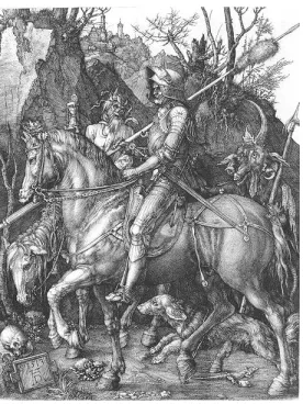
2.2 Albrecht D¨urer Engraving . . . 17
2.3 Lithographic Stone and Print . . . 18
2.4 First Photomechanical Reproduction . . . 19
2.5 The First Photograph . . . 20
2.6 Halftone Photography Process . . . 22
2.7 Digital Halftoning Process . . . 23
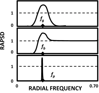
2.8 RAPSD of Halftone Patterns . . . 24
2.9 Campbell-Robson Contrast Sensitivity Target . . . 26
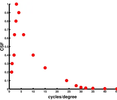
2.10 CSF measured by Campbell and Robson. . . 27
2.11 Comparison of CSF Models. . . 29
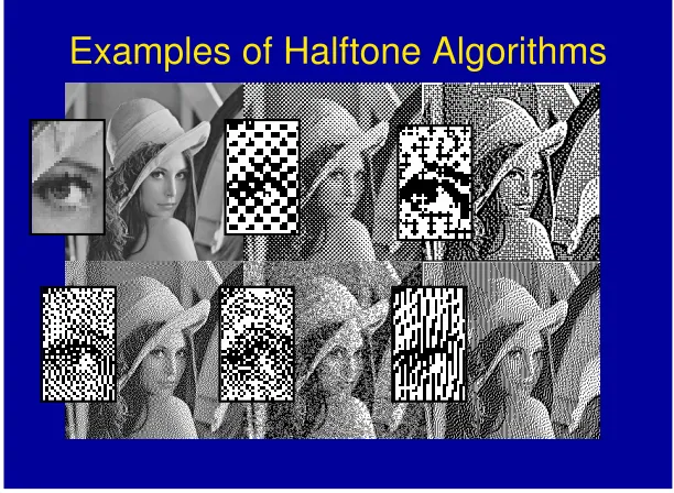
2.12 Examples of Halftone Algorithms . . . 31
2.13 Halftone Algorithm Classification Methods . . . 32
2.14 Halftone Algorithm Strategies . . . 35
2.15 Steps in Electrophotography . . . 38
2.16 Photon paths in a turbid medium . . . 45
2.17 Photon paths in a Printed Substrate . . . 47
2.18 Dot Gain . . . 49
2.19 Dot loss effect . . . 50
2.20 Reflectance vs. Dot Area Fraction for a clustered periodic dot . . 51
2.21 Reflectance variability vs. F : Ideal Printer . . . 53
2.22 Reflectance Variability vs. F: Real Printer . . . 53
2.23 Mean Reflectance vs. dot area fraction with MD equation. . . 57
2.24 Circular Dot Model Parameters. . . 59
2.25 Kacker EP Model. . . 74
2.26 Images with matching histograms . . . 77
2.27 Julesz Conjecture . . . 78
2.28 Steerable Pyramid . . . 83
2.29 Example of a steerable pyramid . . . 84
2.30 Synthesis Algorithm . . . 86
2.31 Diagram of a single Neuron . . . 87
2.32 Diagram of a layer of neurons . . . 88
3.1 Proposed Framework for Electrophotographic Model . . . 93
3.2 Lightness vs. code value . . . 96
4.1 Halftone pattern textures . . . 100
4.2 Variation of texture with gray level . . . 101
4.3 Texture of printed halftones . . . 102
4.4 Pyramid decomposition of an aperiodic clustered halftone pattern 104 4.5 Pyramid decomposition of an aperiodic scan hardcopy print . . . 105
4.6 Subband information of aperiodic halftone dot. . . 107
4.7 Subband information of aperiodic hardcopy print. . . 108
4.10 Measured vs. synthesized parameters for periodic clustered dot . . 112
4.11 Visual comparison of synthesized vs. scanned prints . . . 113
4.12 Visual texture and the normalized euclidian distance . . . 116
4.13 Granularity vs. Euclidian Distance . . . 117
4.14 Marginal statistics vs. image size (N) . . . 121
4.15 Real auto correlation vs. image size (N) . . . 121
4.16 Cousin magnitude correlation vs. image size (N) . . . 122
4.17 Parent magnitude correlation vs. image size (N) . . . 123
4.18 Texture analysis processing time vs. image size (N) . . . 124
4.19 Synthesis as a function of the image size (N). . . 125
4.20 Texture synthesis processing time vs. image size (N) . . . 126
4.21 Texture analysis processing time vs. number of scales (NS) . . . . 127
4.22 Granularity vs. number of scales (NS) . . . 127
4.23 Texture synthesis processing time vs. number of scales (NS) . . . 129
4.24 Texture analysis processing time vs. number of orientations (NO) 130 4.25 Granularity vs. number of orientations (NO) . . . 131
4.26 Texture synthesis processing time vs. number of orientations (NO) 132 4.27 Analysis processing time vs. neighborhood size (Na) . . . 132
4.28 Granularity vs. NA for aperiodic clustered halftone pattern . . . . 133
4.29 Synthesis processing time vs. neighborhood size (NA) . . . 134
4.30 Granularity vs. number of iterations (NI) for aperiodic clustered . 135 5.1 Generalized linear printer model . . . 140
5.2 Scanned vs. linear modeled synthesized images . . . 141
5.4 One hidden layer with 2X neuron FFNN . . . 144
5.5 Large FFNN Results . . . 145
5.6 Large FFNN reflectance mean vs. number of neurons . . . 147
5.7 Large FFNN reflectance variance vs. number of neurons . . . 148
5.8 Large FFNN SNRs vs. number of neurons . . . 149
5.9 Large FFNN SNRs vs. number of hidden layers . . . 150
5.10 Partial parameter synthesis . . . 153
5.11 Granularity SNR for partial parameter synthesis . . . 156
5.12 Granularity SNR for partial parameter synthesis (ALL) . . . 157
5.13 NN architectures studied . . . 158
5.14 SNRs vs. parameters subgroups . . . 159
5.15 Real 2D autocorrelation SNRs vs. parameter subgroups . . . 159
5.16 NNGP1 Modeled vs. measured . . . 161
5.17 NNGP3 Modeled vs. measured . . . 162
5.18 Modeled results for various NN architectures . . . 163
5.19 NNGP4 SNRs vs. number of neurons . . . 164
5.20 NNGP4 SNRs vs. number of hidden layers . . . 165
5.21 SNRs vs. training function . . . 167
5.22 Plot of Table 5.5. . . 170
5.23 Plot of MAC. . . 171
5.24 Plot PMC . . . 172
5.25 Plot CMC . . . 172
5.26 NNGP5 . . . 173
5.27 Modeled textures for various NN architectures . . . 175
5.30 Reflectance Variance vs. Euler Number. . . 178
5.31 NNGP6 . . . 180
5.32 NNGP4 vs. NNGP6 . . . 181
5.33 NNGP4 vs. NNGP6 synthesized images . . . 182
5.34 NNGP4 vs. NNGP6 synthesized images . . . 183
5.35 Dot structure vs. NN architecture . . . 184
5.36 Bank of Neural Networks . . . 185
6.1 Combine clustered periodic dot modeling . . . 187
6.2 Synthesis images of clustered periodic dot modeling . . . 189
6.3 Ellipse fitting. . . 192
6.4 Conceptual dendrogram . . . 194
6.5 Dendrogram of top 30 clusters . . . 197
6.6 Examples of members of two clusters . . . 198
6.7 NNGP6 modeling with morphology training sets . . . 199
6.8 Results of modeling with HPRV and CACR . . . 202
6.9 Bank of Neural Networks (Multiple Algorithms) . . . 203
6.10 NNGP7 Results . . . 204
6.11 SNRS Base vs. New architecture . . . 205
A.1 Original Image. . . 212
A.2 Gaussian Pyramid 4 Levels. . . 212
A.3 Laplacian Pyramid 4 Levels. . . 213
A.4 The steerable Pyramid. . . 214
Introduction
1.1
Motivation
For the past 500 years, printing has been the principal means of conveying ideas.
The influence of printing in social, political, economic, and scientific arenas has
made it a prominent technology in the development of modern civilization. As a
result of a significant number of technological inventions, printing is prevalent and
commonly used, to the point that it has become an everyday commodity in our
homes. One such key inventions was halftoning, because it enabled the automatic
reproduction of images. Halftoning is a printing technology that simulates the
illusion of continuous tone images for printing devices able to deliver only one
level of colorant. The appearance of gray is created by modulating either the
number or the size of printed dots in a given area in proportion to the local
gray tone values. Halftoning works because the human visual system has limited
spatial resolution, which blurs the printed dots of the halftone image, thereby,
creating the gray sensation of a continuous tone image.
that is in close contact with a high contrast film, transforming it into a new film
photograph made of dots of varying sizes [1]. The size of each dot is proportional
to the intensity of the incident light passing through the screen. The new film
photograph is known as a halftone image, and it is used as a mask to transfer the
dot image onto a printing plate.
Digital halftoning is the adaptation of the classical halftoning technology to
digital printing devices such as electrophotographic printers. In digital halftoning,
a digital gray scale image is transformed into a digital image with a discrete
number of tone levels, [2] this is known as multi-level digital halftoning. Binary
halftoning is a special case of multi-level digital halftoning, where the digital
gray scale image is transformed into a bi-level tone digital image by skillfully
controlling the location of the black pixels. The well-defined set of instructions
that control the distribution and location of the black pixels is known as the
digital halftone algorithm [2].
The goal of the digital halftone algorithm is to produce images that, once
printed, are a close reproduction of the original continuous tone image. However,
the printing process is imperfect and introduces distortions to the halftone image,
which needs to be accounted for in the design of the digital halftone algorithms [3].
Due to various physical limitations, the printing process cannot exactly reproduce
the halftone image. At the outset, real printers typically distort the square pixels
into real dots that are relatively round. To completely blacken an area, the
real dots must overlap. This overlapping causes lower gray levels to be perceived
darker than the intended fraction of black dots. Most printers show additional dot
between the aimed and the actual gray level [4]. The quality of the printed
image depends, among other factors, on the interactions between the printer
characteristics, the halftone image, the colorant, and the printing substrate.
Numerous digital halftone algorithms with diverse techniques have been
in-vented, all of them trying to compensate for printing distortions, while keeping
the results within a window where the human visual system does not perceive
artifacts. The first digital halftone algorithms were designed to imitate the
clas-sical screen halftone patterns. For the case of two tone levels, the digital halftone
algorithm converts the intermediate gray level of each pixel of the original gray
scale image into a binary level (0 or 1) to represent a white or a black pixel,
respectively. A common method to assign a binary value to a pixel is based on a
pixel-by-pixel comparison of the original digital image gray values with an array
of threshold values defined within a small selected region (halftone cell) of the
original digital image. Pixels in the halftone image are turned on (printed) if their
value in the original image is larger than its corresponding threshold. To create
the classical halftone dot patterns, the thresholds values within the halftone cell
are arranged to turn-on adjacent pixels along a spiral path, starting from the
center of the array, thereby forming a dot that varies in size according to the
original local gray level. Digital halftoning algorithms that use this modulation
strategy are sometimes called amplitude modulation (AM) halftoning algorithms.
At the time the early digital halftone algorithms were being developed, the printer
resolutions were low. The algorithms assume ideal printers, and did not
incorpo-rate corrections to account for printer distortions. The main concern with AM
halftones was dot visibility. The main goal of the AM halftoning algorithms was
Working with digital images offered additional freedoms when making dot
patterns. As an alternative to amplitude modulation patterns with isolated dots
can be made in order to reduce dot visibility. To obtain isolated dots, the
thresh-old values in the halftone cell can be arranged to turn on non-adjacent pixels
as the gray level increases. In this case, the size of the printed dot is fixed,
but the spacing (frequency) between the printed dots is varied. Digital
halfton-ing algorithms that use this modulation strategy are sometimes called frequency
modulation (FM) halftoning algorithms. The first of the FM halftoning
algo-rithms organized the dots in an ordered arrangement [5, 6]. Algoalgo-rithms that use
the pixel-by-pixel computations, as described above, are sometimes called point
algorithms. Like other halftone algorithms these halftone algorithms also assume
an ideal printer and do not account for printer distortions. However, printers
were still low resolution and the main concern was dot visibility.
There were three problems with digital halftoning algorithms. First, that the
printers needed to have the capability of consistently reproducing isolated dots.
Second, the printed images suffered from a periodic structure that gave them an
artificial appearance. Third, larger tone corrections than AM algorithms were
necessary.
The FM halftoning algorithms were further improved with the algorithm
pro-posed by Floyd and Steinberg [7]. They propro-posed to change the thresholding
computation based on an analysis of the input pixel and its neighbors. These
algorithms are sometimes called neighborhood algorithms. The basic strategy
of the calculation was to distribute the gray error between the original image
this strategy, this algorithm is also known as “Error Diffusion”. Although the
neighborhood calculations considerably increase the computational complexity of
the algorithm, the result was a stochastic pattern of dots that had an apparent
spatial resolution higher than that achieved by the clustered dots of AM.
Ulichney [8] introduced a theory to describe the spatial and spectral
character-istics of the FM patterns. His model was called blue-noise because the frequency
spectrum of the FM dots falls in the high frequencies of halftone patterns, just
like blue light is in the high frequencies of the white light spectrum. The main
problems with the algorithm were; the creation of textures shifts between some
gray levels, recurring unwanted wavy line textures, commonly known as “worms”,
that the amount of tone correction needed was much larger than AM, and that
it required a printer capable of consistently printing isolated dots. A large
num-ber of variations for the basic algorithm have been published [9] pursuing the
elimination of the unwanted textures.
Remarkable improvements in printing technology have been made and as
printers achieve higher resolutions, the capabilities of printing isolated dots from
FM halftoning algorithms is being challenged. This is particularly true for
elec-trophotographic printers. To compensate for printer distortions, researchers
con-tinued to developed numerous variations of digital halftone algorithms. One key
variation was to design halftone algorithms that produce some amount of
clus-tering within the FM algorithms to increase their printing robustness [10, 11, 12].
This type of halftone algorithm is sometimes called AM-FM Hybrid algorithms.
Lau [3, 10] introduced a statistical model to describe the spatial and spectral
characteristics of the AM-FM Hybrid patterns. The new model was called
of the white light spectrum. The green-noise theory describes the ideal
charac-teristics of cluster sizes for a range of cluster sizes. Depending on the printer
reliability, small clusters are restricted for reliable printers while large clusters
are restricted to unreliable printers. The limiting case of this theory is Ulichney’s
blue-noise theory.
With the understanding provided by the green-noise theory, halftone
algo-rithms can be theoretically tuned to the capabilities of the printer. Developing
the halftone algorithm still required finding out what the printer capabilities were.
One common approach to account for the printer capabilities, is to print,
eval-uate, adjust and reprint test samples of the halftone pattern, until a desirable
result is obtained. This requires time, and the availability of judges to complete
the process. An alternative to this process is to construct a printer model that
simulates the printed results. With a printer model, both the cycle time for the
evaluations as well as the number of choices of halftone algorithms can be greatly
reduced.
Implicitly, all digital halftone algorithms assume some form of a printer model.
The digital halftone algorithms that explicitly include a printer model in their
design, are known as model-based digital halftone algorithms [13].
Numerous halftone algorithms have been developed with the implicit
assump-tion of an ideal printer. An ideal printer model assumes that each black dot is
an exact reproduction of the black pixel on the paper. These algorithms required
some form of tone correction. Tone correction is usually a transformation applied
to the image before halftoning. Often this approach does not work well when
non-monotonic, non-linear tonal response. This is particularly noticeable when, FM
algorithms are printed in electrophotographic printers. This is another reason
for developing accurate printer models and for including them in model-based
halftoning algorithms.
Within the model-based algorithms, there is a subclass of algorithms that
uses a numerical optimization strategy to find the optimum halftone image for a
given continuous tone image. These algorithms are usually iterative and typically
aim to minimize the perceived difference between the continuous tone image and
the halftone image. These algorithms are also known as search-based algorithms.
They pursue the ultimate goal of digital halftoning, which is; to optimize the
printing of each image by taking into consideration the interactions between the
image content, the printer characteristics, the toner, and the paper, while doing
this in real time. A common search-based algorithm is the direct binary search
[14, 15]. These algorithms require a human visual system (HVS) model and
printer model. This is another motivation to develop accurate, easy to implement,
printer models.
Numerous electrophotographic printer models with a variety of modeling
tech-niques have been invented. Some of the early work in modeling the paper light
scattering effects on the printed reflectance can be interpreted as printer
mod-els. One of the early approaches was the Yule-Nielssen model [16], in which a
power function is fitted to actual measured reflectance data to model the printed
reflectance. Various modifications to this equation have been done to account
for the interactions between the printer and the halftone pattern interactions
[17, 18, 19]. The limitations of such a model are: numerous parameters need to
tion shapes can be fitted.
Another popular approach toward printer modeling is to simulate the print
dot as a hard circular dot. The goal of this model is to estimate the average gray
value of the printed pixel as a function of the halftone pattern bitmap based on
the amount of overlap of the dots in the neighborhood of the pixel. There are
also various modifications to the basic model, including some for which, instead
of calculating gray values with a formula, a table of gray values is created from
actual measurements of each possible dot pattern configuration in the
neighbor-hood. This approach has been accurate for many printers but cannot describe all
printer behaviors, so it requires different models for different printer technologies
and different printer resolutions. The interactions between the dots can be very
complex and this type of model does not have the power to model them.
The most complex electrophotographic printer models are those that attempt
to describe the physical behavior of each step in the printing process, also known
as physics-based models. For electrophotographic printers, these models tend to
be mathematically complex because they model the dynamics of the printer
sub-processes. These models also require significant knowledge of the specific printer
design parameters, and are also very difficult to implement.
A variation of the physics-based model describes the printer sub-processes in
a static, rather than in a dynamic way [20, 21]. These models are still
mathemat-ically complex although some of the steps could be modeled as a linear system.
Unfortunately, they still require detailed knowledge of the specific printer
param-eters, are difficult to implement, therefore, are not very portable.
They model the probability of getting a toner particle developed at a given
posi-tion, as a function of the distance to the center of the exposure. To account for
dot interactions, they calculate the total exposure at the point, including
neigh-boring exposures. These models assume that the printers have a single toner
efficiency transfer function. The dot structures calculated by these models are
similar to the actual dot structures. The main drawbacks of the models are: that
they require the estimation of the printer toner efficiency transfer function, and
that they do not account for the stochastic dot shape variations of the printer.
Kacker et al. [22] developed another electrophotographic printer model in
which he calculated an exposure to absorptance curve for the printer. The
expo-sure is calculated from an analytical description of the laser beam profile which
includes the capability of modulating the laser exposure time. To calibrate the
model for a specific printer, he printed a special set of halftone patterns that
re-sults in negligible dot gain. The exposure to absorptance curve that he developed
is claimed to be a printer function. To calibrate for a specific halftone pattern,
a series of constant gray patches are printed and their absorptance is measured.
These measurements are used to adjust the printer function for dot gain. The
ex-posure to absorptance curves are used to estimate the specific absorptance of the
possible dot arrangements and they are implemented as a look-up table. Some
drawbacks of this model are: that detailed knowledge of the printer parameter
are required, and that two calibrations and a look-up table need to be calculated.
Another semi-empirical approach to printer modeling is Nielssen’s, in which
the halftone pattern is interpreted as a toner coverage map. In this model, a
physical spread function is convolved with the halftone pattern to simulate the
printer, by including a tone transfer function like Lau [3], and by developing a
technique to measure the amount of toner in a printed sample. The model did not
perfectly reproduce the printing process, particularly for FM and AM-FM hybrid
dots. This model requires the estimation of a physical point spread function, a
noise function, a toner transfer function, and a toner coverage calibration.
All of the above printer models have been useful in specific or limited
appli-cations. The more complex models have been more suitable for use by the
com-munity of printer designers. The simpler ones have been more suitable for AM
algorithms printed in low resolution printers. From this brief review of
electropho-tographic printer models, it is clear that some of the most common drawbacks of
current printer models are: their dependence on printer technology, complexity
of calculations, complexity of calibration, that they do not account for all types
of printer distortions, and that they are halftone pattern dependent.
To advance the halftone algorithm technology, some desirable characteristics
of an electrophotographic printer model are that they: need to account for all
types of printer distortions, need to minimize computational complexity, are
de-signed to be printer technology independent, are dede-signed for ease of calibration,
and for minimizing halftone pattern dependence. The current frameworks for
building electrophotographic printing models do not meet all desired
character-istics listed above. This research was motivated by the need to explore new
approaches for improved printer modeling.
The two research objectives of this dissertation are (1) to introduce a new
framework for printer modeling and (2) to demonstrate the feasibility of such
framework introduces the concept of modeling a printer as a texture
transfor-mation machine. The basic premise is that modeling the texture differences
be-tween the output printed images and the input images, encompasses all printing
distortions including; the printer characteristics, the input halftone image, the
colorants, and the substrate. This approach offers a new viewpoint in printer
modeling research with the potential of addressing the shortfalls of current
mod-els.
1.2
Contributions
A key contribution of this thesis was the introduction of a new type of printer
model for electrophotographic printers. The model was based on the premise
that an electrophotographic printer is a texture transformation machine. A
ba-sic framework from which printer models can be built in a texture space was
presented, and its feasibility was demonstrated. A second contribution was the
implementation of the printer model framework as a bank of feed-forward neural
networks. The key texture parameters to be modeled by the bank were identified.
It was also demonstrated that the set of input texture parameters was insufficient
for accurate modeling and as an additional contribution a set of topology
param-eters that augmented the set was identified, thereby improving the accuracy of
the results. A third contribution was the establishment of guidelines for the
oper-ational limits of the multiresolution operoper-ational parameters. Another key
contri-bution of this thesis was the development of a method to select training sets based
on the classification of the morphological properties of the halftone patterns. The
development of this method was instrumental when modeling multiple halftone
pattern granularity.
The printer model framework is fast, and has the capability to continue to
learn with additional training. The model is also simple to implement because it
only requires a calibrated scanner. The model was tested with halftone patterns
representing a wide range of spatial characteristics found in halftoning. Our
re-sults show that our model provides accurate predictions for marginal statistics
and granularity. When trained with a set of mixed halftone patterns, the model
performed well with minimal failures. Our implementation is only one of many
possible implementations for the proposed framework. Results demonstrate
sig-nificant accuracy. Further research in this area is warranted to continue the
development of printer models in a texture space.
1.3
Organization
Chapter 2 reviews various technologies that are relevant to this research. The
chapter begins with a historical review of printing technology from the perspective
of solving the image reproduction problem. The review spans from early
man-ual reproduction techniques to the current digital halftoning techniques. Then
the fundamental principles of the electrophotographic printing technology are
reviewed. The imperfections of the printing process with emphasis on the
elec-trophotographic process are presented. The next section examines the literature
of printing models with emphasis on to electrophotographic process. An
introduc-tion to visual texture follows with emphasis on the statistical theory of texture.
The chapter ends with an introduction to neural networks.
based on the premise that a printer is a texture modifying machine. This chapter
describes the basic architecture of the printer model.
In Chapter 4 the concept of a halftone pattern texture is reviewed and tested.
The study includes the parametric texture representation of the halftone patterns,
the feasibility of the parametric representation for printer modeling, an evaluation
of the texture space, and sensitivity studies to identify a practical operating range
and combination of the analysis and synthesis parameters.
Chapter 5 describes the implementation of the framework in the form of a
neural networks printer model. The identification of key modeling parameters
and the concept of a bank of neural networks is also described in this chapter.
Chapter 6 expands the work of the previous chapter to include modeling
independent of halftone algorithm. This chapter introduces a morphological
clas-sification method for halftone patterns that is use for the selection of training
sets.
Chapter 7 presents the conclusions of this research and discusses numerous
Background
Chapter 2 reviews various technologies relevant to this research. The chapter
begins with a historical review of printing technology (§2.1) from early manual
reproduction techniques to current digital halftoning techniques. The review is
from the perspective of techniques used to solve the image reproduction
prob-lem. Section 2.2 reviews fundamental principles of electrophotographic printing
technology. Section 2.3 reviews the imperfections of the printing process with
emphasis on electrophotographic printers. Section 2.4 examines the literature of
printing models with emphasis on the electrophotographic process. An
introduc-tion to visual texture follows (§2.5) focusing on the statistical theory of texture.
The chapter ends with an introduction to the basics of neural networks (§2.6).
2.1
Printing
For the past 500 years, printing has been the principal means of conveying ideas.
The influence of printing in social, political, economic, and scientific arenas has
made it a prominent technology in the development of modern civilization.
Print-ing allowed knowledge to spread among the populace instead of keepPrint-ing it confined
to elite groups. Nowadays, printing is prevalent and commonly used; it has
be-come an everyday commodity in our homes. This was not the case a few decades
ago, until a number of significant technological inventions were developed.
Specif-ically, image reproduction technologies were needed because reproducing images
is more complex than printing text. For example, consider the task of creating
a black and white printed image of a scene. Each position in the scene has an
intensity level with values in a continuous range from white to black. However,
each equivalent position in the printed image has only two intensity levels; either
to cover the area with black colorant, resulting in a completely black spot, or to
leave the area uncovered resulting in a white spot. Printing a midtone gray is
not an option. This constraint is known as the image reproduction problem and
results from the fact that the density of the black colorant cannot be changed. To
solve the image reproduction problem, clever printing techniques were invented
in order to give the appearance of the mid-level gray tones.
2.1.1
Early Manual Image Reproduction Techniques
One of the earliest image reproduction techniques, known as xylography1, was
developed in China (c.500) and consisted of skillful hand carvings of scenes in
wood blocks (Figure 2.1). Artists knew that the human eye had limited spatial
resolution and that a gray sensation could be created by controlling the number,
thickness, and orientation of the carved lines. Printing was done by inking the
face of the wood block and bringing it in contact with the paper. The back of
1
reproduced images were crude, using only coarse lines.
Figure 2.1: Chinese wood block print page from the Diamond Sutra (the earliest known book bearing an actual date) printed c.868 during the Tang Dynasty. (Image source:Wikimedia Commons, US public domain)
Improvements in carving tools and cutting techniques resulted in printed
im-ages of better quality. However, by the 16th century the limitations of wood block
printing had been reached. Wood blocks were carved with finer detail than could
be reproduced in the print. Further improvements in image reproduction were
achieved around the 17th century with the invention of other printing techniques,
such as Intaglio2. Intaglio is a printing technique in which a design is engraved
into a metal plate, ink is forced into the cut lines and wiped off the rest of the
surface, damp paper is laid on top, and both plate and paper are rolled through
a press. The use of metals, such as copper, further increased the quality of the
prints because it allowed for greater precision in the cutting technique by use of
2
fine needles or chemical etching. The intaglio process was commonly used for fine
illustrative work. One of the great masters of woodcuts and intaglio was Albrecht
D¨urer, who tried to turn the print medium into an art form. A famous example
[image:37.612.250.388.237.421.2]of his art is shown in Figure 2.2.
Figure 2.2: Albrecht D¨urer, Knight,Death and the Devil copper engraving in the Mu-seum Boijmans van Beuningen collection. (Image source: Wikimedia Commons, US public domain)
In 1796, Alois Senefelder invented a printing method based on the repulsion of
oil and water. In this innovative method, an oil-based image is put on the surface
of a smooth piece of limestone, acid is added to etch the image onto the surface,
a water soluble solution is then applied which sticks only to the non-oily surfaces
and seals it. The stone is covered with an oily ink which will only adhere to the
oily part of the image; paper is laid on top to transfer the ink. Because the original
method involved a piece of limestone, this method was named lithography3. An
3
Figure 2.3: Lithographic Stone and Print of an old map of Munich. (Wikimedia Com-mons image from Chris 73. License under the creative commons cc-by-sa 2.5 license)
Because engraving was tedious and required a skillful craftsman, images were
expensive to reproduce and; Therefore, pictures were sparsely used even with the
advent of the printing presses. In a typical process, an artist would make a sketch
of the scene, followed by a more detailed drawing. The drawing would be copied,
sometimes in reverse, onto a smooth block of wood. A craftsman would then cut
away all of the surface but the lines to be printed. The finished block would then
be pressed into clay, making an impression of the image. Molten metal was then
2.1.2
Photomechanical Reproduction
Around 1822, Joseph Nicephore Niepce discovered that the asphalt compound,
known as bitumen of Judea, previously used to control acid etching in the intaglio
process, had two remarkable properties. This material would bleach to a light
gray color upon exposure to sunlight, and it would also selectively harden in
the exposed areas. He used this material to produce the first photomechanical
reproduction of a paper engraved image of the Cardinal d’Amboise. Niepce coated
a pewter plate with the bitumen of Judea, and exposed it by placing it in contact
with the paper engraving which had been previously oiled to make the paper
almost transparent. The light passing through the clear areas of the engraving
hardened the bitumen to the plate, while the unexposed areas remained soluble.
After dissolving the soluble areas, he treated the plate in an acid bath to etch the
uncovered metal in the location of the engraving lines, creating a printing plate
(Figure 2.4).
from the third floor window of his house at Le Gras, by placing the coated pewter
plate inside a camera obscura (Figure 2.5).
Figure 2.5: Reproduction of the first permanent photograph, view from the window at Le Gras, created by Niepce in 1826. Due to the long sunlight exposure the buildings are illuminated from both sides. (Image source: Wikimedia Commons, US public domain)
The photomechanical process for intaglio printing developed further, with
modifications that resulted in the plate’s etched cavities being proportional to
the intensity of the exposed light. When photography came into use in the 1840s
it did not immediately alter printing. The fundamental limitation of the
print-ing process still existed; only solid blacks and whites could be rendered. The
intermediate shades of gray found in a photograph could not be reproduced. At
that time, photography supported the intaglio engraving process by replacing the
artist’s sketch of the scene with a photograph. The image quality of photography
greatly exceeded the quality of any printed image of that time. However,
pho-tographs could not be reproduced in mass quantities. Only exclusive books had
realized until techniques for transferring photographs to print were invented.
2.1.3
Halftoning
In 1852, the limitation of printing photographs was overcome when William Fox
Talbot, after experimenting with screens and gauze, invented the halftone
pho-tography process [24].
Halftone photography is an imaging process that exposes an original film
pho-tograph through a screen (Figure 2.6), onto a high contrast film that effectively
thresholds the screened image, transforming it into a new film photograph made
of halftone dots of varying sizes. The size of each dot is proportional to the
inten-sity of the incident light passing through the screen. The new film photograph is
known as a halftone image and it is used as a mask to transfer the dot image onto
a printing plate. The impact of this discovery was not fully realized until almost
forty years later, when the first halftone photographic reproductions appeared in
daily newspapers (c.1890).
The halftoning process was further developed by the Levy brothers in 1893,
when they patented the first commercial screen [25]. The screen consisted of two
glass plates with cross-hatched opaque lines forming transparent squares which
produced sharp edged dots (hard dots). The next breakthrough occurred in
1953 with Hepher’s invention of the contact screen [1]. The contact screen is a
photographic film exposed and processed with a vignette pattern. This screen is
put in close contact with a high contrast photographic media to produce a halftone
image with dots with diffused edges (soft dots). Numerous modifications of the
contact screen continue to evolve, contributing to the development of the graphic
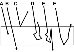
Figure 2.6: Halftone photography process. Light reflected from the original image A passes through the halftone screen B and exposes a high contrast film C resulting in a halftone image. The size of each dot is proportional to the intensity of the incident light. The halftone image is use as a mask to the dot image onto a printing plate D.
Nowadays, most halftone images are digitally generated.
2.1.4
Digital Halftoning
Digital halftoning is the process of converting a continuous tone image into a
pattern of pixels with a discrete number of tone levels using digital processing
techniques [2, 27]. The pattern of pixels, also known as the halftone image, is
used to display the continuous tone image in media incapable of reproducing
continuous tones. The most familiar example is the printing of ink or toner onto
paper (Figure 2.7). For bi-level printers, each position in the printed image has
only two choices: to cover the area with ink, resulting in a black spot or to leave
to a well-defined set of instructions for transforming a continuous tone image into
a discrete number of tone levels so that it can be printed. The goal of the digital
halftone algorithm is to produce images that once printed are a close reproduction
of the original continuous tone image.
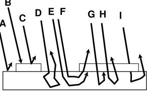
Figure 2.7: Digital Halftoning Process. The original digital contone image A is pro-cessed by the halftone algorithm B resulting in the halftone image C which is propro-cessed by the printer D to generate a replicate E of the original image.
2.1.4.1 Definition of Halftone Patterns
In the context of this research, halftone patterns will be defined as the binary
images resulting from the application of a halftone algorithm to a constant tone
field. Sometimes halftone patterns are referred to as halftone textures. In many
halftone algorithm design processes, halftone patterns are created and printed so
during printer characterizations. Halftone patterns are used as targets because
the quality of a printed image depends on the interaction between the printer
characteristics and the halftone pattern, among other factors.
The spatial frequency content of the halftone patterns, often characterized
by the Noise Power Spectrum (NPS), is sometimes used to classify the halftone
patterns. The shape of the radially average NPS, also known as the radially
av-erage power spectrum density (RAPSD) is used to broadly classify the halftone
patterns into three groups: green-noise, blue-noise, and periodic-noise halftone
patterns (Figure 2.8). The color terminology used is an analogy to the color of
[image:44.612.228.401.367.528.2]
Figure 2.8: RAPSD of the ideal green, blue, and periodic-noise halftone patterns. The RAPSD is shown relative to the white-noise RAPSD, which is represented as the dotted straight line. Thefg, fb,and thefpare the principal frequencies for each halftone
pattern. (Adapted from [28])
the light that has a similar frequency spectrum as that of the halftone pattern.
intermediate frequencies. Blue-noise halftone patterns are those that have most
of the noise power at high frequencies with almost no low frequency components.
Periodic-noise halftone patterns are those that have their noise power
concen-trated at a given frequency. Figure 2.8 shows a comparison of the RAPSD of
the ideal green, blue, and periodic-noise halftone patterns. The RAPSD is shown
relative to the white-noise RAPSD, which is represented as the dotted straight
line. The fg, fb,and thefp are the principal frequencies for each halftone pattern.
NPS is also used as a classification method to categorize halftone algorithms as
discussed below in section 2.1.4.3.
2.1.4.2 Perception of Halftones
How a printed image is perceived depends on the interaction of the printer
charac-teristics, the halftone image, the substrate (commonly paper), and the
character-istics of the HVS [29, 16]. One of the key charactercharacter-istics of the HVS that governs
the perception of the printed image, is it’s inability to detect small differences
between shades of gray as the spatial frequency increases [30]. The difference
in brightness between two shades of gray is known as the image contrast.
Con-trast is measured as the ratio of the difference between the luminances of the two
gray levels, and their sum. This is shown in Equation 2.1, where Lmax and Lmin
represent the luminances of the two gray levels.
C = Lmax−Lmin
Lmax+Lmin
(2.1)
The contrast sensitivity of the HVS can be experienced by observing the
Campbell-Robson contrast sensitivity target shown in Figure 2.9. The target
Figure 2.9: Campbell-Robson Contrast Sensitivity Target. Image source: PostScript program c1996 Izumi Ohzawa. See [31, 32, 33, 34, 35]
contrast along the y-axis [31]. The viewer can experience the difficulty of
detect-ing low contrasts in the rightmost (higher spatial frequencies) and the leftmost
(lower spatial frequencies) sections of the target. The decrease in sensitivity at
higher frequencies and low frequencies is due to various factors including the
lateral inhibition of ganglion cells, the optical characteristics of the cornea and
lens, and the result of the eye adapting to a large range of lighting conditions.
The function that describes the contrast sensitivity of the HVS is known as the
contrast sensitivity function (CSF) [30, 36]. The CSF provides guidelines for the
resolution requirements of a printer and for the acceptable range of spatial
fre-quencies for the halftone images. It also allows for the development of metrics
that measure the distortion seen by a human viewer.
The CSF has been measured for the average observer with carefully designed
0 5 10 15 20 25 30 35 40 45 0
0.1 0.2 0.3 0.4 0.5 0.6 0.7 0.8 0.9
cycles/degree
[image:47.612.215.413.123.292.2]CSF
Figure 2.10: Contrast Sensitivity Function (CSF) measured by Campbell and Robson.
Robson [31]. The figure shows that the CSF is a bandpass function with peak
sen-sitivity from 3 to 10 cycles/deg. Approximately beyond 40 cycles/deg, the viewer
cannot distinguish the high frequencies and sees only gray. For example, given
that a square wave grating can be made of an infinite sum of the odd harmonics
of sine wave components, then any square grating above 13.5 cycles/deg will have
its next harmonic above 40 cycles/deg, which is outside the resolution limit of the
HVS. For reference, the acuity of 20/20 vision is defined as 30 cycles/deg. The
interpretation is that, to print a high contrast square grating, the printer needs
to be able to reproduce sharp edges to a resolution equivalent to 13.5 cycles/deg,
while a single sinusoidal response (first harmonic) is adequate between 13.5 to 40
cycles/deg. Equation 2.2 converts the distance independent units of cycles/deg
to printer resolution units of lines/inch for a given viewing distance. In Equation
2.2, Pr is the printer resolution in lines/in, d is the distance in inches, and fθ
is the spatial frequency in cycles/deg. For a viewing distance of 12 inches, the
Pr=
dtan
1
2fθ
−1
(2.2)
The CSF has been extensively reported in the literature as the visual transfer
function (VTF) or modulation transfer function (MTF) of the eye. To facilitate
the implementation of the CSF, several models have been proposed. Table 2.1
and Figure 2.11 illustrate three models that have been used in the development
of halftone algorithms. The Campbell [37] and the Mannos [38] models are
band-pass, while the Daly model [39], is lowpass. The lowpass behavior of the Daly
model accounts for the fact that viewers do not keep a fixed distance from the
image. The model allows low frequencies that are more visible at larger viewing
distances to pass. To apply these models to a specific viewing distance, the
angu-lar frequency has to be related to a spatial frequency through Equation 2.3, where
fl is the spatial frequency in cycles/mm,fθ is the spatial frequency in cycles/deg,
and d is the viewing distance in mm.
fl=
180
π arcsin
1
√
1 +d2
fθ (2.3)
One additional consideration in modeling the HVS is to account for the fact
that eye sensitivity depends on the orientation of the observed features. The
eye is less sensitive to the detection of slanted features than to the detection
of horizontally or vertically oriented features. To account for this behavior, the
CSF models are transformed using equation 2.4, wherefr is the radial frequency,
θ = arctan(fy
fx) is the angle between the horizontal (fx) and the vertical (fy)
frequencies,s(θ) is a function that represents the angular dependence of the HVS,
andCSF(fr, θ) is the angular corrected CSF. Daly proposeds(θ) = 0.15 cos(4θ)+
Model Model Parameters
Campbell e−2παfθ −e−2πβfθ α = 0.012, β = 0.046
Mannos α(β+γfθ)e−(γfθ)
δ α= 2.6, β = 0.0192
γ = 0.114, δ= 1.1
Daly
α(β+γfθ)e−(γfθ)
δ
if fθ > fθmax
1 else
α= 2.6, β = 0.192
γ = 0.114, δ= 1.1
fθmax = 6.6
Table 2.1: Models for the CSF
0 10 20 30 40 50
0 0.1 0.2 0.3 0.4 0.5 0.6 0.7 0.8 0.9 1
fθ (cycles/deg)
CSF
Campbell Mannos Daly
CSF(fr, θ) =CSF
fr
s(θ)
(2.4)
The CSF models allow for the development of metrics to measure the
distor-tion of the halftone image as seen by a human viewer. For example, when printing
a uniform shade of gray (flat field) using two different halftone algorithms, the
distortions as seen by a human viewer can be calculated as the root mean square
error between the original continuous tone image and the binary halftone image
after filtering with the CSF.
2.1.4.3 Halftone Algorithm Classification
After years of research, numerous halftone algorithms with diverse techniques
have been invented with various levels of success in reproducing the original
contone image (Figure 2.12). Today, halftone algorithm development continues
to be an active research area [1, 2]. Concurrent with the development of the
halftone algorithm techniques, various ad hoc classification methods came into
use, in part with the objective to fulfill the need of predicting the print quality of
a given halftone algorithm and printer combination. The classification methods
evolved informally from the perspective of different authors, inevitably resulting
in overlapping classifications, none of which is recognized as a standard. Following
is a review of the main classifications methods reported in the literature, other less
commonly used classification methods are discussed in review articles by Stoffel
[41] and by Jones [42].
The halftone algorithm classification methods are organized under two
ba-sic viewpoints: the dot distribution viewpoint and the dot generation viewpoint
com-Examples of Halftone Algorithms
Figure 2.13: Halftone Algorithm Classification Methods
monly used classification methods: the dot organization method, and the dot
power spectrum method. The first method (Dot Organization) classifies halftone
algorithms according to the organization and size of the dots. In this method,
the halftone algorithms are first broadly categorized as a clustered or dispersed
dot [3, 4]. In clustered dot halftone algorithms, the tone levels are represented
by aggregating neighboring pixels in the digital halftone image therefore, forming
a growing cluster of pixels that print as a larger dot. Modulating the size of
the dot cluster controls the density of the halftone pattern. The digital halftone
algorithms that use this technique are often referred to as amplitude modulated
(AM) halftones, since it is the size or amplitude of the dot that is modulated
(Figure 2.14). In contrast, in dispersed dot halftone algorithms, the tone level is
each other to represent each gray level [7, 8]. In this case, the density level of
the halftone pattern is controlled by modulating the number of the dots that are
turned on. These types of halftone algorithms are often referred to as frequency
modulated (FM) halftones since it is the number or frequency of the printed dots
rather than the size of the dot what is modulated (Figure 2.14).
The clustered dot and the dispersed dot categories are further subdivided
ac-cording to whether the halftone dots are placed in a periodic (ordered) or an
ape-riodic (irregular) pattern [6, 7], hence resulting in four classification groups.
Oc-casionally, the terms hybrid dot [8] or micro clustered [9] are associated with the
aperiodic-cluster-dot category. Hybrid dot halftone algorithms are often viewed as
a combination of the AM and FM types because the pixels are grouped into small
clusters and these clusters are maintained as far as possible from each other. The
result is local clusters of dots that are globally dispersed [12](Figure 2.14).
Repre-sentative halftoning algorithms for each of the groups are: centered-clustered dot
periodic) [2, 8], Bayer (dispersed-periodic) [5], microcluster
(clustered-aperiodic) [43], and error diffusion (dispersed dot-(clustered-aperiodic) [7].
The second classification method under the dot distribution viewpoint (Dot
Power Spectrum) classifies halftone algorithms according to the halftone dots
noise power spectrum. This type of halftone pattern classification was
previ-ously discussed in Section 2.1.4.1 and is now applied to the halftone algorithm.
The main classification method has three categories; blue-noise, green-noise,
and periodic-noise. Representative halftoning algorithms for each of the groups
are; error diffusion (blue-noise) [7], linear pixel shuffling (green-noise) [44], and
centered-clustered dot (periodic-noise)[2, 8].
screens, and computation type. The first method (Computational Screens)
clas-sifies halftone algorithms into two main groups, adaptive and non-adaptive, based
on the computation method used [45]. The non-adaptive category refers to
al-gorithms that use computationally designed halftone screens, while the adaptive
category refers to halftone algorithms that perform direct calculations on the
input image. Arguably, the non-adaptive category also performs direct
calcula-tions on the input image (e.g. thresholds the image). However, to belong to the
non-adaptive category, the halftone algorithms must also compute each pixel
in-dependently of its neighbors and must accomplish this in a single computational
path on the input image. All halftone algorithms that do not meet the three
non-adaptive criteria are classified as adaptive. The adaptive category is further
subdivided into two subcategories, iterative and iterative. The adaptive
non-iterative category includes algorithms that complete only one path of calculations
on the continuous tone input image. The adaptive iterative algorithms are those
that carry out multiple paths of calculations on the continuous tone input image
until some pre-defined error criterion is minimized. Representative halftoning
algorithms for each of the categories are: all the screen thresholding algorithms
(non-adaptive), Floyd-Steingberg error diffusion (adaptive non-iterative) [7], and
direct binary search (adaptive iterative) [14, 15].
The second classification method under the dot generation viewpoint,
classi-fies halftone algorithms according to the type of computation performed on the
continuous tone input image. The halftone algorithms are further sub-divided
into three main categories: point, neighborhood, and iterative. The point
image is a function of only one pixel of the continuous tone input image. In the
neighborhood algorithm category, each pixel of the halftone image is a function
of a local neighborhood of the continuous tone image. In the iterative algorithm
category, the final halftone image is attained after several passes of calculations
through the continuous tone image. In the halftone literature, these categories
are also occasionally referred to as: screening (point), error diffusion
(neighbor-hood), and model-based (iterative). Representative halftoning algorithms for each
of the categories are; clustered dot (point) [2, 8], Floyd-Steingberg error diffusion
[7](neighborhood), and direct binary search [14, 15].
Figure 2.14: Halftone algorithm dot distribution strategies. The top row shows three gray levels of an AM halftone. The middle row show the same three gray levels for an FM halftone, the bottom row show the same three gray levels for a Hybrid halftone
In practice, the current halftone algorithm classification methods have limited
utility because they only provide a vague idea of what the printed output quality
might be. Recent progress in understanding the interaction between the binary