Full-scale unsteady RANS CFD simulations of ship behaviour
and performance in head seas due to slow steaming
Tahsin Tezdogan
n, Yigit Kemal Demirel, Paula Kellett, Mahdi Khorasanchi, Atilla Incecik,
Osman Turan
Department of Naval Architecture, Ocean and Marine Engineering, Henry Dyer Building, University of Strathclyde, 100 Montrose Street, Glasgow G4 0LZ, UK
a r t i c l e i n f o
Article history: Received 30 July 2014 Accepted 24 January 2015
Keywords: Seakeeping CFD
Fully nonlinear motion simulations Added resistance
Slow steaming Full-scale KCS
a b s t r a c t
It is critical to be able to estimate a ship's response to waves, since the resulting added resistance and loss of speed may cause delays or course alterations, with consequentfinancial repercussions. Slow steaming has recently become a popular approach for commercial vessels, as a way of reducing fuel consumption, and therefore operating costs, in the current economic and regulatory climate. Traditional methods for the study of ship motions are based on potentialflow theory and cannot incorporate viscous effects. Fortunately, unsteady Reynolds-Averaged Navier–Stokes computations are capable of incorpor-ating both viscous and rotational effects in theflow and free surface waves. The key objective of this study is to perform a fully nonlinear unsteady RANS simulation to predict the ship motions and added resistance of a full scale KRISO Container Ship model, and to estimate the increase in effective power and fuel consumption due to its operation in waves. The analyses are performed at design and slow steaming speeds, covering a range of regular head waves, using a commercial RANS solver. The results are validated against available experimental data and are found to be in good agreement with the experiments. Also, the results are compared to those from potential theory.
&2015 The Authors. Published by Elsevier Ltd. This is an open access article under the CC BY license (http://creativecommons.org/licenses/by/4.0/).
1. Introduction
Understanding the behaviour of a vessel in a real seaway is critical for determining its performance. Rough sea conditions induce significant ship motions, which affect a ship's resistance. The resulting increase in resistance can compromise propulsive efficiency and can increase fuel consumption. Ship motions and seakeeping behaviour are also very important with regards to crew, vessel and cargo safety. An awareness of the impacts of ship motions on resistance is particularly important in the current economic climate, which has seen a significant increase in fuel costs in comparison to charter rates. For example, for a typical commercial vessel, the fuel costs will now account for well over half of its operating costs, whereas for a container ship, thefigure may be as high as 75% (Ronen, 2011).
The current economic climate is very different from the“boom years” in which modern vessels were designed. In response to recent fuel price increases, ship operators have begun to apply the slow steaming approach, which was initially proposed by Maersk technical experts post-2007 (Maersk). In this approach, a vessel is
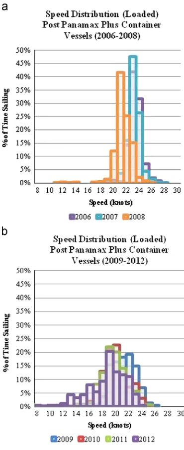
operated at a speed significantly below its original design speed in order to reduce the amount of fuel that is required. Slow steaming is typically defined as being down to around 18 knots for container vessels, with operational speeds below this being termed‘super slow steaming’.Fig. 1, taken fromBanks et al. (2013), shows how the operating speeds for container vessels have decreased over recent years, comparing the period from 2006–2008 with 2009–
2012. It can be seen that a typical operating speed is now significantly below the original design speeds which would have been specified for these vessels. In particular, it can be observed that for this collection of data, the most typical slow steaming speed is around 19 knots. This speed will therefore be used as a representative slow steaming speed in this study.
Other concepts such as“just-in-time”operation and virtual arrival are also applied as a means of reducing speed without compromising the agreed dates for charter cargo delivery into port. In some cases, vessels are even retro-fitted with lower power propulsion systems to reduce weight and improve efficiency, as well as reduce the problems which may arise from the long-term operation of machinery in off-design conditions. However, little research has been carried out into the effect that these lower speeds may have on the behaviour of the vessel, and whether further fuel savings may be an additional benefit. This paper addresses the gap in current knowledge by comparing Contents lists available atScienceDirect
journal homepage:www.elsevier.com/locate/oceaneng
Ocean Engineering
http://dx.doi.org/10.1016/j.oceaneng.2015.01.011
0029-8018/&2015 The Authors. Published by Elsevier Ltd. This is an open access article under the CC BY license (http://creativecommons.org/licenses/by/4.0/).
nCorresponding author. Tel.:þ44 1415484912.
pitch and heave motions, as well as added resistance, at both design and slow steaming speeds. More importantly, although extensive research has been performed to investigate increases in effective power, ship fuel consumption and CO2emissions, no specific study
exists which aims to predict the increase in the above mentioned parameters due to the operation in waves, using a Computational Fluid Dynamics (CFD)-based Reynolds Averaged Navier–Stokes (RANS) approach. Therefore, the main aim of this study is to directly predict the increase in the required effective power of a vessel operating in regular head seas. This leads to a rough estimation of the fuel penalty to counter the additional CO2emissions from the vessel.
The potential benefits of slow steaming will be probed by invoking added resistance predictions.
The Energy Efficiency Operational Indicator (EEOI) was intro-duced by the International Maritime Organisation (IMO) in 2009 as a voluntary method for monitoring the operational performance of a ship. The EEOI enables an assessment to be made of the operational energy efficiency of a ship, which is expressed in terms of the CO2 emitted per unit of transport work (IMO, 2009).
Alongside this, regulations relating to the control of SOxemissions
from shipping were introduced, with specific limits stipulated. This will be followed by limits for NOxemissions in 2016, with
limits for CO2and particulate matter (PM) emissions also likely to
be introduced in the future. Reducing the fuel consumption through slow steaming, and improving or at least maintaining propulsive efficiency, will take steps towards addressing these requirements.
The resistance of a ship operating in a seaway is greater than its resistance in calm water. The difference between these two resistances arises from ship motions and wave drift forces in waves and has been termed the added resistance due to waves. Added resistance can account for up to 15–30% of the total resistance in calm water (Pérez, 2007). It is therefore critical to be able to accurately predict the added resistance of a ship in waves, and this should be included in ship performance assessments. One purpose of this study is to predict the added resistance due to waves with higher accuracy than potential theory-based methods.
The KRISO Container Ship (KCS), developed by the Korean Mar-itime and Ocean Engineering Research Institute (now MOERI), has been used in a wide range of research studies. There is consequently a wide range of experimental and simulation data available for compar-ison, and for verification and validation purposes. The KCS has there-fore been investigated in this study due to the ready availability of this data and research in the public domain. Moreover, container ships are particularly affected by slow steaming, as they were designed to operate with very high design speeds, in the region of up to 25 knots. The service speed for KCS is 24 knots. This makes the KCS model particularly relevant for this study.
As discussed by the International Towing Tank Conference (ITTC) (2011a), advances in numerical modelling methods and increases in computational power have made it possible to carry out fully non-linear simulations of ship motions, taking into account viscous effects, using CFD. In this study, an unsteady RANS approach is applied using the commercial CFD software Star-CCMþ version 9.0.2, which was developed by CD-Adapco. Addi-tionally, the supercomputer facilities at the University of Strath-clyde have been utilised to allow much faster and more complex simulations.
A full-scale KCS hull model appended with a rudder is used for all simulations, to avoid scaling effects. The model wasfirst run in calm water conditions free to trim and sink so that the basic resistance could be obtained, for both the design and the slow steaming speeds. The model was then run in a seaway, to allow the ship motions to be observed and to allow the added resistance due to waves to be calculated. This was again carried out for both speeds in question. The resistance was monitored as a drag force on the hull, and the pitch and heave time histories were recorded. This paper is organised as follows. Section 2 gives a brief literature review on seakeeping methods and the implementation of RANS methods for the solution of seakeeping problems. After-wards, the main ship properties are given, and a list of the simulation cases applied to the current CFD model is introduced in detail inSection 3. Next, inSection 4, the numerical setup of the CFD model is explained, with details provided in the contained sub-sections. Following this, all of the results from this work, including validation and verification studies, are demonstrated and discussed inSection 5. Finally, inSection 6, the main results drawn from this study are briefly summarised, and suggestions are made for future research.
2. Background
[image:2.595.74.259.55.508.2]The vast majority of the available techniques to predict ship motions, as well as the added resistance due to waves, rely on assumptions from potential flow theory, including free surface
Fig. 1.Comparison of the speed distributions for container vessels, taken from
effects. However, many previous studies such asSchmitke (1978)
have shown that viscous effects are likely to be the most significant, particularly in high amplitude waves and at high Froude numbers.
Beck and Reed (2001)estimate that in the early 2000s, 80% of all seakeeping computations at forward speeds were performed using strip theory, owing to its fast solutions. Another advantage of strip theory is that it is applicable to most conventional ship geometries. On the other hand, as discussed byNewman (1978), the conventional strip theories are subject to some deficiencies in long incident waves and at high Froude numbers. This is thought to be caused by the evolution of forward speed effects and the complex nature of the diffraction problem.Faltinsen and Zhao (1991)also state that strip theory is questionable when applied at high speeds, since it accounts for the forward speed in a simplistic manner. Discrepancies between strip theory and experiments for higher speed vessels, or highly non-wall sided hull forms, have therefore motivated research to develop more advanced theories, such as the 3-D Rankine panel method, unsteady RANS methods and Large Eddy Simulation (LES) methods (Beck and Reed, 2001).
As computational facilities become more powerful and more accessible, the use of 3-D techniques to study seakeeping pro-blems is becoming more common. As explained in detail by
Tezdogan et al. (2014a),Yasukawa (2003)claims that 3-D methods have been developed to overcome the deficiencies in the strip theory methods. In the method developed by Bertram and Yasukawa (1996), full 3-D effects of theflow and forward speed are accounted for, in contrast to strip theory where these effects are not properly taken into account.Yasukawa (2003)applied the theory of Bertram and Yasukawa (1996) to several container carriers with strongflare. As a result of his study, it was reported that hydrodynamic forces, ship motions and local pressures are much better predicted using the theory ofBertram and Yasukawa (1996)than the results obtained by strip theory when compared to experiments. However, the predicted lateral hydrodynamic forces are not satisfactory, due to the viscous flow effect. Yasukawa (2003)suggests that this problem can be diminished by applying empirical corrections, similar to those employed in strip theory.
Simonsen et al. (2013)highlight that the effects which are ignored in the potential theory such as breaking waves, turbulence and viscosity should be directly taken into account in the numerical methods. RANS methods, for instance, are very good alternatives to the potential flow theory as they can directly incorporate viscous effects in their equations.
Continued technological advances offer ever-increasing com-putational power. This can be utilised for viscousflow simulations to solve RANS equations in the time domain. CFD-based RANS methods are rapidly gaining popularity for seakeeping applica-tions. These methods have the distinct advantage of allowing designers to assess the seakeeping performance of a vessel during the design stages, therefore allowing any corrective action to be taken promptly, before the vessel is actually built (Tezdogan et al., 2014b).
In 1994, a CFD workshop was organised in Tokyo to discuss the implementation of steady RANS methods to provide a solution for free-surface flows around surface ships. As explained byWilson et al. (1998), from that point onwards, RANS methods have been widely used in many marine hydrodynamics applications.
As discussed by Simonsen et al. (2013), RANS-based CFD methods have been used extensively for seakeeping performance analyses with several ship types, by many scholars. Sato et al. (1999) conducted CFD simulations to predict motions of the Wigley hull and Series 60 models in head seas. Hochbaum and Vogt (2002)then performed simulations of a C-Box container ship in 3 degrees-of-freedom motions (surge, heave and pitch) in head seas. Following this, Orihara and Miyata (2003) predicted the
added resistance and pitch and heave responses of the S-175 container ship in regular head seas, using the Baldwin–Lomax turbulence model. In their work, they investigated the effect of two selected bulbous forms on the predicted added resistance.
CFD simulations have been also performed for more complex ship geometries.Weymouth et al. (2005), for example, simulated the pitch and heave motions of a Wigley hull in regular incoming waves.Carrica et al. (2007)studied the motions of a DTMB 5512 model in regular, small amplitude head waves.Hu and Kashiwagi (2007)also investi-gated the pitch and heave responses of a Wigley hull in head seas.
Stern et al. (2008)studied the pitch and heave responses of BIW-SWATH in regular head waves.Wilson et al. (2008)and Paik et al. (2009) performed CFD simulations to predict the pitch and heave transfer functions of the S-175 ship in regular head waves.Carrica et al. (2008)demonstrated an application of an unsteady RANS CFD method to simulate a broaching event for an auto-piloted ONR Tumblehome in both regular and irregular seas. Then, Castiglione et al. (2011)
investigated the motion responses of a high speed DELFT catamaran in regular head waves at three different speeds. Following this,
Castiglione et al. (2013)carried out CFD simulations for seakeeping of the same catamaran model at two Froude numbers in both head and oblique regular waves.
Bhushan et al. (2009)performed resistance and powering compu-tations of the full-scale self-propelled Athena ship free to sink and trim using both smooth and rough wall functions. They also carried out seakeeping simulations at both full and model scale along with manoeuvring calculations for DTMB 5415 at full-scale.Mousaviraad et al. (2010)obtained heave and pitch response amplitudes and phases of the DTMB 5512 model in head seas using regular wave and transient wave group procedures. Following this, Simonsen and Stern (2010)performed CFD RANS simulations to obtain the heave and pitch motions and added resistance for the KCS model, presenting it at the Gothenburg 2010 CFD workshop. In addition,Enger et al. (2010) contributed to the same workshop with their study on the dynamic trim, sinkage and resistance analyses of the model KCS by using the Star-CCMþsoftware package. In their work, it was demon-strated that the CFD results agreed well with the experimental results. Following this, Carrica et al. (2011)presented two computa-tions of KCS in model scale, utilising CFDShip-Iowa, which is a general-purpose CFD simulation software developed at the Uni-versity of Iowa. They performed self-propulsion free to sink and trim simulations in calm water, followed by pitch and heave simulations in regular head waves, covering three conditions at two different Froude numbers (Fn¼0.26 and 0.33). Then, Kim (2011)carried out CFD analyses for a 6500 TEU container carrier, focusing on the global ship motions and structural loads by successfully validating the results against the model test measure-ments. After the validation study, Kim (2011) claimed that the current CFD technology would facilitate the decision making process in ship optimisation. Finally, Simonsen et al. (2013)
investigated motions,flow field and resistance for an appended KCS model in calm water and regular head seas by means of Experimental Fluid Dynamics (EFD) and CFD. They focused mainly on large amplitude motions, and hence studied the near resonance and maximum excitation conditions. The results obtained using the CFD methods were compared to those from their experiments and the potentialflow theory method.
To the best of our knowledge, the majority of RANS seakeeping simulations have been performed at model scale. However, as
Hochkirch and Mallol (2013)claim, model-scaleflows and full-scale
stern flow reveals that these scale effects are not negligible and depend strongly on the stern geometries”. As discussed in detail with several examples byHochkirch and Mallol (2013), performing analyses at a full scale is of the greatest importance, especially for hulls appended with propulsion improving devices (PIDs). A decision was therefore made to use the full-scale KCS model in the CFD simulations presented in this paper.
In addition, during this literature review, it was seen that when using the KCS model, although resistance predictions have been conducted for a range of Froude numbers (for exampleBanks et al., 2010 and Enger et al., 2010), seakeeping analyses have only been performed at forward speeds corresponding to a Froude number of 0.26 or higher (for exampleSimonsen et al., 2013 and Carrica et al., 2011). This study therefore may be useful to understand the seakeeping behaviour and performance of the KCS model at a slow steaming speed.
3. Ship geometry and conditions
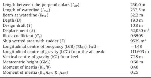
A full scale model of the KCS appended with a rudder was used within this study. The main properties of the KCS model are presented inTable 1(Kim et al., 2001):
As stated previously, the service speed for this vessel is 24 knots (12.345 m/s). A slow steaming speed of 19 knots (9.773 m/s) was selected as a representative value for current container ship operations.
The CFD simulations were performed at twelve different con-ditions, as listed inTable 2, each identified by their case numbers. The frequency of encounter of the waves fe is calculated by fe¼
ffiffiffiffiffiffiffiffiffiffiffiffiffiffiffiffiffi g=ð2
πλ
Þ pþU=
λ
for head seas (wheregdenotes the gravita-tional acceleration, and Udenotes the ship forward speed). The waves were selected such that the ratio of wave over ship length varied between 1 and 2. Also, the wave steepness in all cases was chosen to be 1/60, in a similar manner to the experiments ofSimonsen et al. (2013). It is also of note that the analyses were performed using deep water conditions.
Resonance occurs when the frequency of encounter of wavesfe
equals, or, is close to, the natural frequency of the shipfn. For the
present full-scale model, the natural heave and pitch frequencies were computed to be close tofn¼0.124 Hz based on the
calcula-tions given bySimonsen et al. (2013). Case 3 was therefore chosen to be investigated more closely in the verification study.
The excitation forces and moments are dependent on the ratio of wave length over ship length.Simonsen et al. (2013)state that the maximum excitation force for the KCS occurs for wave lengths close to
λ
/LBP¼1.33. Case 4 is the condition in which the maximumexcitation force is expected to occur.
Case 6, according to the work byCarrica et al. (2011), exhibits a very linear behaviour since the wavelength is very large. It can hence be regarded as the most linear condition amongst all of the cases.
4. Numerical modelling
Up to this point, this paper has provided a background to this study and has given an introduction to the work. The following section will provide details of the numerical simulation approaches used in this study and will discuss the numerical methods applied to the current CFD model.
4.1. Governing equations
For incompressibleflows without body forces, the averaged con-tinuity and momentum equations may be written in tensor form and Cartesian coordinates as follows (Ferziger and Peric, 2002):
∂
ρ
ui
∂xi ¼
0 ð1Þ
∂
ρ
ui ∂t þ∂ ∂xj
ρ
uiujþ
ρ
u0iu0j
¼ ∂∂xp iþ
∂
τ
ij∂xj ð
2Þ
in which
τ
ijare the mean viscous stress tensor components, as shownin Eq.(3)
τ
ij¼μ
∂ ui ∂xjþ∂uj ∂xi
ð3Þ
andpis the mean pressure,uiis the averaged Cartesian components of
the velocity vector,
ρ
u0iu0jis the Reynolds stresses,ρ
is thefluid density andμ
is the dynamic viscosity.To modelfluidflow, the solver employed uses afinite volume method which discretises the integral formulation of the Navier–
Stokes equations. The RANS solver employs a predictor–corrector approach to link the continuity and momentum equations.
4.2. Physics modelling
The turbulence model selected in this study was a standardk–
ε
model, which has been extensively used for industrial applications (CD-Adapco, 2014). Also,Querard et al. (2008)note that the k–
ε
model is quite economical in terms of CPU time, compared to, for example, the SST turbulence model, which increases the required CPU time by nearly 25%. Thek–
ε
turbulence model has also been used in many other studies performed in the same area, such asKim and Lee (2011)andEnger et al. (2010).
[image:4.595.44.290.617.745.2]The “Volume of Fluid” (VOF) method was used to model and position the free surface, either with aflat or regular wave.CD-Adapco (2014)defines the VOF method as,“a simple multiphase model that is well suited to simulating flows of several immiscible fluids on numerical grids capable of resolving the interface between the mixture's phases”. Because it demonstrates high numerical efficiency, this model is suitable for simulatingflows in which each phase forms a large structure, with a low overall contact area between the different phases. One example of suchflow is the sloshing of water in a tank, during which the free surface remains perpetually smooth. If the movement of the tank becomes stronger, then breaking waves, air bubbles in the water and airborne water droplets will form as a result. The VOF model uses the assumption that the same basic governing equations as those used for a single phase problem can be solved for all thefluid phases present within the domain, as it is assumed that they will have the same velocity, pressure and temperature. This means that the equations are solved for an equivalentfluid whose properties represent the different phases and their respective volume fractions (CD-Adapco, 2014). The inlet velocity and the volume fraction
Table 1
KCS general properties.
Length between the perpendiculars (LBP) 230.0 m
Length of waterline (LWL) 232.5 m
Beam at waterline (BWL) 32.2 m
Depth (D) 19.0 m
Design draft (T) 10.8 m
Displacement (Δ) 52,030 m3
Block coefficient (CB) 0.6505
Ship wetted area with rudder (S) 9539 m2 Longitudinal centre of buoyancy (LCB) (%LBP), fwdþ 1.48 Longitudinal centre of gravity (LCG) from the aft peak 111.603 m Vertical centre of gravity (KG) from keel 7.28 m
Metacentric height (GMt) 0.60 m
Moment of inertia (Kxx/B) 0.40
of both phases in each cell, as well as the outlet pressure are all functions of theflat wave or regular wave used to simulate the free surface. The free surface is notfixed, it is dependent on the specifi ca-tions of this flat or regular wave, with the VOF model making calculations for both the water and air phases. The grid is simply refined in order to enable the variations in volume fraction to be more accurately captured. In this work, a second-order convection scheme was used throughout all simulations in order to accurately capture sharp interfaces between the phases.
Fig. 2demonstrates how the free surface was represented in this CFD model by displaying the water volume fraction profile on the hull. In thefigure, for instance, a value of 0.5 for the volume fraction of water implies that a computational cell isfilled with 50% water and 50% air. This value therefore indicates the position of the water–air interface, which corresponds to the free surface.
It should also be mentioned that in the RANS solver, the segregated
flow model, which solves theflow equation in an uncoupled manner, was applied throughout all simulations in this work. Convection terms in the RANS formulae were discretised by applying a second-order upwind scheme. The overall solution procedure was obtained accord-ing to a SIMPLE-type algorithm.
In order to simulate realistic ship behaviour, a Dynamic Fluid Body Interaction (DFBI) model was used with the vessel free to move in the pitch and heave directions. The DFBI model enabled the RANS solver to calculate the exciting force and moments acting on the ship hull due to waves, and to solve the governing equations of rigid body motion in order to re-position the rigid body (CD-Adapco, 2014).
4.2.1. Choice of the time step
The Courant number (CFL), which is the ratio of the physical time step (
Δ
t) to the mesh convection time scale, relates the meshcell dimension
Δ
xto the meshflow speedUas given below:CFL¼U
Δ
Δ
tx ð4Þ
The Courant number is typically calculated for each cell and should be less than or equal to 1 for numerical stability.
Often, in implicit unsteady simulations, the time step is determined by theflow properties, rather than the Courant number. In order to gain a suitable level of accuracy within a reasonable running time, two different time step resolutions were used based on the features of each simulation.
For resistance computations in calm water, the time step size is determined by
Δ
t¼0.005–0.01L/U(whereLis the length between perpendiculars) in accordance with the related procedures and guidelines ofITTC (2011b).For the prediction of ship responses to incident regular waves, at least 100 time steps per encounter period were used, as recommended byITTC (2011b).
It is also worth noting that a first-order temporal scheme was applied to discretise the unsteady term in the Navier–Stokes equations.
4.3. Computational domain and boundary conditions
Two different computational domains were created for each main simulation: a seakeeping analysis in waves and a resistance calculation in calm water.
In both domains, an overset mesh was used to facilitate the motions of the full-scale ship model. Rigid and deforming mesh motion options are available in the software package, but these methods have distinct disadvantages compared to the overset mesh approach when simulating bodies with large amplitude
Table 2
The cases to which the CFD model is applied.
Case no. Ship speed (kn) Froude number Wave height (m) Wave length (m) Encounter period (s) Encounter freq. (Hz) Wave steepness Wave/ship length
C U Fn H λ Te fe H/λ λ/LBP
1 24 0.260 Calm water
2 3.833 230.000 7.349 0.136 1/60 1.00
3 4.424 264.494 8.097 0.124 1/60 1.15
4 5.108 306.480 8.956 0.112 1/60 1.33
5 5.750 345.000 9.704 0.103 1/60 1.50
6 7.689 460.000 11.751 0.085 1/60 2.00
7 19 0.206 Calm water
8 3.833 230.000 8.008 0.125 1/60 1.00
9 4.424 264.494 8.789 0.114 1/60 1.15
10 5.108 306.480 9.684 0.103 1/60 1.33
11 5.750 345.000 10.460 0.096 1/60 1.50
12 7.689 460.000 12.578 0.080 1/60 2.00
The bold rows inTable 2indicate the conditions which were used for the validation of the CFD results against the available experimental results. Each case highlighted in bold has significantly different features, and was purposely selected to be used during the later validation stage. The validation and verification can be found inSection 5.1.
motions. The rigid motion approach causes difficulties for free surface refinement, especially in pitch, and deforming meshes may lead to cell quality problems. On the other hand, the overset region, which encompasses the hull body, moves with the hull over a static background mesh of the whole domain (Field, 2013). For this reason, using the overset mesh feature of the software package saves computational costs, and allows the generation of a sufficiently refined mesh configuration around the free surface and the body, without compromising the solution's accuracy. Without the use of the overset mesh feature, simulating a full-scale ship model in waves would require a very high cell number, requiring much more computational power.
In all CFD problems, the initial conditions and boundary conditions must be defined depending on the features of the problem to be solved. The determination of these boundary conditions is of critical importance in order to be able to obtain accurate solutions. There are a vast number of boundary condition combinations that can be used to approach a problem. However, the selection of the most appropriate boundary conditions can prevent unnecessary computational costs when solving the pro-blem (Date and Turnock, 1999).
When using the overset mesh feature, two different regions were created to simulate ship responses in waves, namely back-ground and overset regions. A general view of the computation domain with the KCS hull model and the notations of selected boundary conditions are depicted inFig. 3.
In order to reduce computational complexity and demand, only half of the hull (the starboard side) is represented. A symmetry plane forms the centreline domain face in order to accurately simulate the other half of the model. It should be noted that in some figures given hereafter, the mirror image of the ship and domain is reflected on the port side for plotting purposes.
Fig. 3illustrates that a velocity inlet boundary condition was set in the positive x direction, where incident regular waves were generated. The negative xdirection was modelled as a pressure outlet. The top and bottom boundaries were both selected as velocity inlets. The symmetry plane, as the name suggests, has a symmetry condition, and the side of the domain (the negativey
direction) has a velocity inlet boundary condition as well. These boundary conditions were used as they were reported to give the quickestflow solutions for similar simulations carried out utilising Star-CCMþ (CD-Adapco, 2014). The use of the velocity inlet boundary condition at the top and the side of the background prevents the fluid from sticking to the walls. In other words, it avoids a velocity gradient from occurring between thefluid and the wall, as in the use of a slip-wall boundary condition. It is of note that the initialflow velocity at all inlet conditions was set to the corresponding velocity of the head waves. Hence, theflow at
the very top and very side of the background is also directed parallel to the outlet boundary. This enablesfluid reflections from the top and side of the domain to be prevented. In addition to this, the selection of the velocity inlet boundary condition for the top and bottom facilitate the representation of the deep water and infinite air condition, which is also the case in open seas. The top, bottom and side boundaries could have been set as a slip-wall or symmetry plane. The selection of boundary conditions from any appropriate combination would not affect the flow results sig-nificantly, provided that they are placed far enough away from the ship hull, such that theflow is not disturbed by the presence of the body. Also, the pressure outlet boundary condition was set behind the ship since it prevents backflow from occurring andfixes static pressure at the outlet.
Date and Turnock (1999)point out that, just as the selection of the boundaries is of great importance, their positioning is equally important. It has to be ensured that no boundaries have an influence on theflow solution.
ITTC (2011b)recommends that for simulations in the presence of incident waves, the inlet boundary should be located 1–2LBP
away from the hull, whereas the outlet should be positioned 3–
5LBPdownstream to avoid any wave reflection from the boundary
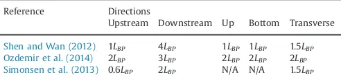
walls. Three other pieces of previous work similar to this study have also been consulted to decide the locations of the boundaries. Thefindings are summarised inTable 3.
The locations of the boundaries are illustrated inFig. 4, which gives front and side views of the domain. It is worth mentioning that throughout all the cases, in order to prevent wave reflection from the walls, the VOF wave damping capability of the software package was applied to the background region with a damping length equal to 1.24LBP (285 m.). This numerical beach model
was used in downstream, bottom and transverse directions. It should be noted that in CFD applications with ship models, there are no definite recommendations regarding how to define the dimensions of an overset region. In this study, the dimensions of the overset region were defined such that the most significant flow features, for exampleflow separation, slamming, wave breaking and high vortices around the hull, remained within the overset domain.
As outlined previously, for the resistance simulations in calm water, another computational domain was created. The only difference from the domain created to simulate ship motions in waves is that the outlet boundary was located 2.5LBPaway from the ship body, as wave
reflection from the walls was less prominent. Irrespective of this, the waves generated by the presence of the vessel were treated by applying a numerical damping beach in each boundary. It should be stated that the boundary conditions in the domain for the simulations in calm water were identical to the ones depicted inFig. 3.
4.4. Coordinate systems
Two different coordinate systems were adopted to predict ship performance in waves. Firstly, theflowfield was solved, and the excitation force and moments acting on the ship hull were calculated in the earth-fixed coordinate system. Following this, the forces and moments were converted to a body local coordinate system which was located at the centre of mass of the body,
Velocity Inlet
Velocity Inlet
Velocity Inlet Velocity Inlet
Pressure Outlet
No-Slip Wall Overset Region
Symmetry
[image:6.595.315.561.685.744.2]Fig. 3.A general view of the background and overset regions and the applied boundary conditions.
Table 3
The locations of the boundaries in similar previous studies.
Reference Directions
Upstream Downstream Up Bottom Transverse
Shen and Wan (2012) 1LBP 4LBP 1LBP 1LBP 1.5LBP
Ozdemir et al. (2014) 2LBP 3LBP 2LBP 2LBP 2LBP
following the motions of the body whilst the simulation pro-gressed. The equations of motions were solved to calculate the vessel's velocities. These velocities were then converted back to the earth-fixed coordinate system. These sets of information were then used tofind the new location of the ship and grid system. The overset grid system was re-positioned after each time step (Simonsen et al., 2013). Information about the ship geometry and the position of the centre of gravity were provided inSection 3.
4.5. Mesh generation
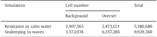
Mesh generation was performed using the automatic meshing facility in STAR-CCMþ, which uses the Cartesian cut-cell method. Two different mesh generations were applied for each resistance and seakeeping simulation, resulting in a computation mesh of circa 4 and 10 million cells in total, respectively. A trimmed cell mesher was employed to produce a high-quality grid for complex mesh generating problems. The ensuing mesh was formed pri-marily of unstructured hexahedral cells with trimmed cells adja-cent to the surface. The breakdown of the mesh number for each resistance and seakeeping simulation is shown inTable 4. It should be noted that the data contained inTable 4for the‘seakeeping in waves’simulation reflects the exact number of grids generated for Case 3. The cell number of the other cases differs slightly from those listed in the table, due to variation in the wave conditions.
The computation mesh had areas of progressively refined mesh size in the area immediately around the hull and rudder, as well as the expected free surface and in the wake that was produced by the ship, to ensure that the complexflow features were appro-priately captured. The refined mesh density in these zones was achieved using volumetric controls applied to these areas. The mesh was unstructured, rigid and body-fixed, so that motions of the body corresponded to the movement of grid points. The most refined mesh areas around the hull remained within the bound-aries of the overset domain. When generating the volume mesh, extra care was given to the overlapping zone between the back-ground and overset regions.CD-Adapco (2014)can be consulted for any further information as to how to generate suitable meshes when working with the overset mesh feature.
To simulate ship motions in waves, the mesh was generated based on the guidelines for ship CFD applications from ITTC (2011b). According to these recommendations, a minimum of 80
cells per wavelength should be used on the free surface. As suggested byKim and Lee (2011), in order to capture the severe free surfaceflows such as slamming and green water incidents, a minimum of 150 grid points per wavelength was used near the hull free surface in both downstream and upstream directions. Additionally, a minimum of 20 cells was used in the vertical direction where the free surface was expected.
When generating the mesh for the simulations in calm water, the refined mesh area for the free surface was kept relatively small, compared to that used in the seakeeping simulations. In this case, based on prior experience, a minimum cell size of 0.0785% of
LBPin the vertical direction was used to capture theflow features
in the free surface.
Fig. 5shows a cross-section of the computation mesh where the refinement to capture the Kelvin wake is clearly visible.Fig. 6
shows the surface mesh on the KCS hull and rudder. The overset mesh region around the hull is also noticeable inFig. 5.
4.6. Post-processing formulations
Before moving on to the results and discussion, it is first necessary to explain the formulations used during the processing of the results.
To begin with, Fourier Series (FS) were used to analyse the unsteady time histories of the force and motions due to waves. Each unsteady history
φ
(t) can be represented by a Fourier Series in time, as given by:φ
ðtÞ ¼φ
0þ XNn¼1
φ
nU cosð2π
fentþγ
nÞ; n¼1;2;3;… ð5Þwhere
φ
nis thenth harmonic amplitude andγ
nis the [image:7.595.38.553.59.270.2]correspond-ing phase. These values can be calculated uscorrespond-ing the followcorrespond-ing
[image:7.595.300.554.331.391.2]Fig. 4.The dimensions of the computational domain for the seakeeping simulations (a) Front view, (b) Side view (B: half beam of the ship, D: depth of the ship, L: length of the ship between the perpendiculars).
Table 4
The cell numbers for resistance and seakeeping simulations.
Simulation Cell number Total
Background Overset
expressions:
φ
n¼ffiffiffiffiffiffiffiffiffiffiffiffiffiffiffi a2
nþb 2 n q
ð6aÞ
γ
n¼arctan bnan ð
6bÞ
in which,
an¼
2
T Z T
0
φ
ðtÞcosð2
π
fentÞdt ð7aÞbn¼
2
T ZT
0
φ
ðtÞsinð2
π
fentÞdt ð7bÞIn these equationsTdesignates the encounter period of waves. The 0th harmonic amplitude
φ
0in FS is defined as the averagevalue of the time history of
φ
(t), which can be obtained as follows:φ
0¼1
T Z T
0
φ
ðtÞdt ð8Þ
The first FS harmonic
φ
1 refers to the linear term from theunsteady histories. Hence, the zeroth andfirst FS harmonics have been named as the fundamental components in the linear system. In particular, taking precedence from previous studies, we focused on the 0th and 1st order terms for the force and motions, as they are used for the calculation of resistance and transfer functions (TF), respectively (Shen and Wan, 2012). During the post proces-sing of the quantities, it was observed that for the resistance in waves, higher order terms have significant effects. This observa-tion has also been reported in the literature. For example,
Simonsen et al. (2013) claim that for the resistance in waves, second and third order FS terms may make up to 50% and 15% of thefirst order FS amplitude, respectively. For any further details regarding the higher order terms, reference can be made toOtzen and Simonsen (2010).
The ship motions in waves were quantitatively analysed with transfer functions. The definition of heave and pitch transfer functions, respectively, can be given by:
TF3¼ x31
ζ
I1 ð9Þ
TF5¼ x51
k
ζ
I1 ð10Þ
where x31, x51 and
ζ
I1 are the first FS harmonic amplitudes ofheave, pitch, and incident wave time histories, respectively, and
k¼2
π
/λ
is the wave number. It must be highlighted that in this work, the heave and pitch motions were evaluated at the ship's centre of gravity.For calm water and for wave conditions, the dimensionless total resistance coefficientCTwas used to analyse the total resistance of
a ship.CTis calculated by:
CT¼ FX
ð1=2Þ
ρ
U2S ð11ÞwhereFXis the X-force measured in the global coordinate system
(the total resistance) and S is the wetted area of the vessel in calm water.
The added resistance due to waves was calculated by first subtracting the calm water resistanceFX,calmfrom the 0th FS harmonic
amplitude of the X-force in waves (FX,wave) at the same ship speed. It
was then non-dimensionalised, as follows:
σ
aw¼ðFX;waveFX;calmÞ
ρ
gζ
2I1B 2 WL=LBPð12Þ
σ
aw, given in the above equation, has been termed the addedresistance coefficient. The added resistance of the vessel due to waves will be presented by giving the added resistance coefficients over the wave/ship length ratios at both speeds.
5. Results and discussion
The following section will outline the simulation results achieved during this study, and will also provide some comparison with experimental results and the results from potential flow theory. It will then present a discussion on the observation of the results. This section is divided intofive main sub-sections, each of which presents different aspects of ourfindings. Before proceeding to examine the results obtained, it isfirst necessary to validate the current CFD approach against the experimental results.
5.1. Validation and verification
Due to the large body of data available for the KCS, it is possible to use experimental data for comparison with the simulated results. This can then be used to validate the approach and results.
5.1.1. Ship resistance in calm water
The total resistance (drag) of a shipRTis mainly composed of
two components; the residuary resistance RR and the frictional
resistanceRFas given by Eq.(13)(Gillmer and Johnson, 1982).
RT¼RRþRF ð13Þ
Eq. (13) can also be expressed in its more common non-dimensional form. This is achieved by dividing each term by the denominator of Eq.(11). Hence, the total resistance coefficientCTis
made up of the residuary resistance coefficientCRand the frictional
resistance coefficientCF. Given that the residuary resistance coeffi
-cient is a function of the Froude number (Fn), and the frictional resistance coefficient is a function of the Reynolds number (Re), the total resistance coefficient can, therefore, be written in the following form (Schultz, 2007):
CT¼CRðFnÞþCFðReÞ ð14Þ
The frictional resistance coefficientCF, for both model and full-scale
ships, can be found by using the following ITTC-1957 formula:
CF¼
0:075
ðlog10Re2Þ
[image:8.595.49.289.58.176.2]2 ð15Þ
Fig. 5.A cross-section of the computation mesh showing the refined mesh to capture the Kelvin wake.
[image:8.595.41.291.232.439.2]The Reynolds number at a ship speed of 24 knots for the full-scale KCS model is calculated to be 2.839109.
Ship resistance can be predicted through towing tank tests conducted with a ship model which is geometrically similar to the full-scale ship. To predict the resistance of the full-scale ship using the model test results, a dynamic similarity has to be achieved between the model and the full-scale ship.
In our CFD simulations, the full-scale model was initially towed in calm water conditions free to trim and sink at a speed of 24 knots (Case 1). After the solution had converged adequately, the last twenty seconds ofFxtime history were used for the Fourier analysis. The 0th
FS harmonic of the total resistance coefficient was calculated to be 2.2945103 by our CFD model. During the towing tank tests conducted bySimonsen et al. (2013)at a model speed of 1.701 m/s, which corresponds to 24 knots in full scale, the coefficients of total resistance and residuary resistance for a 1/52.667 scale model of the KCS (Remodel¼6.517106) were found to be 4.310103 and
1.064103, respectively. In order to make a comparison to our case,
the full scale CTs value was predicted to be 2.414103 from the
model tests. It should be highlighted that the towing tank experiments were also conducted in trim and sinkage free conditions.
As can clearly be seen from the above calculations, theCTvalue of
the vessel in calm water at 24 knots is quite compatible with the experiments, and is only under-predicted by 4.95% compared to the towing tank results.
5.1.2. Wave generation
5th-order Stokes waves were used inside the computational domain throughout all simulations. The theory of the 5th-order wave is based on the work byFenton (1985). The reason for selecting this wave is that according toCD-Adapco (2014),“this wave more closely resembles a real wave than one generated by thefirst order method”. The first order wave mentioned here is the wave that generates a regular periodic sinusoidal profile.
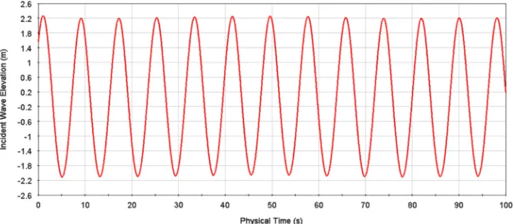
To monitor the waves generated at the inlet, a wave probe was used to record the wave elevation in each case.Fig. 7illustrates the
position of the wave probe between the inlet and vessel.Fig. 8, as an example, displays the recorded time history of the wave elevation at the probe in Case 3.
By applying FS on a window of the time series of the wave elevation shown inFig. 8, the mean of the 1st harmonic wave amplitudes covering the last ten periods of encounter was calcu-lated to be 2.140 m, which under-predicts the actual wave ampli-tude (2.212 m) by 3.23%. This slight reduction of the wave amplitude was found to be acceptable for the current cell size and time step, and was sufficiently reasonable for the validation of wave generation by the current CFD model.
5.1.3. Wave pattern
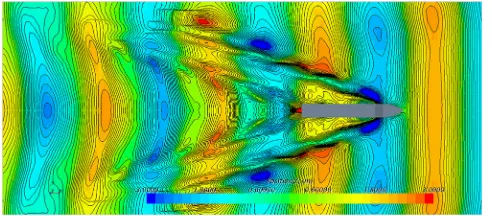
Case 3 was selected as a representative case to show both the wave contours and the motions of the vessel.Fig. 9 shows the global wave pattern around the KCS when the solution was initialised, andFig. 10 shows the same plot after the simulation has completed its run. The Kelvin wake generated by the ship is clearly visible inFig. 10.
In order to visualise bow motions of the vessel in waves, four snapshots of the waves and the bow movement of the vessel were taken in a period of encounter and are displayed inFig. 11. The
figure expressly shows that breaking bow waves and the slamming incident have been successfully captured by the current CFD model. It is noteworthy to mention that the snapshots in the
figure were recorded after the motions reached steady-state. In addition to this, an animated version of Fig. 11 is provided in Electronic Annex I.
Supplementary material related to this article can be found online athttp://dx.doi.org/10.1016/j.oceaneng.2015.01.011.
5.1.4. Ship motions and added resistance
As was mentioned inSection 3, three pre-selected different cases in waves were used for the validation of the CFD model against experiments. In this sub-section, heave and pitch as well asCThistories
of the vessel in each simulation will be given in detail and the results will then be compared to the available experimental and CFD data obtained by previous studies.
[image:9.595.37.280.454.544.2]Simonsen et al. (2013), as mentioned inSection 2, also investigated the KCS by means of EFD and CFD. They used CFDShip-Iowa as the RANS solver in all of their simulations, and Star-CCMþ for several specific simulations. Ultimately, they compared all of their CFD results to experimentalfindings. For this reason, our results for Cases 3 and 4 were compared to their CFD and EFD results. Also, for Case 6, we benefited from the CFD work ofCarrica et al. (2011), who performed computations with CFD Ship-Iowa. They compared their results with the experimental study ofOtzen and Simonsen (2010), as well as with
Fig. 7.Numerical wave probe (the white line) to record the wave elevation.
[image:9.595.112.475.573.731.2]the CFD results of several researchers, who used different numerical approaches.
Table 5presents a comparison of the heave and pitch transfer functions between the current CFD model and the other CFD simulations performed by other researchers, as well as the related experimental data. The comparison error (E), which is defined as the difference between the experimental data and the calculated
data, is also included in the table. It should also be mentioned that inTable 5, the pitch responses are given in radians.
The total resistance coefficients obtained are given inTable 6and are compared only to the EFD data, since all the other available CFD simulations were performed with a model scale KCS. However, the full-scaleCTsvalues by EFD were predicted from the model tests in
order to make a precise comparison with the experiments, for reasons discussed in the previous sub-section.
FromTable 5, it can be seen that for heave transfer functions, the current CFD model predicts within 0.42–9.39% of EFD, and for
[image:10.595.47.293.309.417.2]Fig. 9.Measured wave pattern around the KCS hull when the simulation is initialised.
[image:10.595.139.467.472.735.2]Fig. 10.Measured wave pattern around the KCS hull after the simulation has completed its run.
Fig. 11.Four snapshots of wave patterns and bow movements of the vessel in a given period of encounter. Table 5
The transfer functions in the validation study.
Case no. TF3 TF5
3 EFD (Simonsen et al., 2013) 0.950 0.693
CFDShip-Iowa (Simonsen et al., 2013) 0.995 0.769
Error (% of EFD) 4.74 10.97
Star-CCMþ(Simonsen et al., 2013) 0.861 0.731
Error (% of EFD) 9.37 5.48
The Current CFD 0.946 0.664
Error (% of EFD) 0.42 4.18
4 EFD (Simonsen et al., 2013) 1.107 0.971
CFDShip-Iowa (Simonsen et al., 2013) 0.950 0.959
Error (% of EFD) 14.18 1.24
The Current CFD 1.003 0.895
Error (% of EFD) 9.39 7.83
6 EFD (Otzen and Simonsen, 2010) 0.901 1.037 CFDShip-Iowa (Carrica et al., 2011) 0.854 0.993
Error (% of EFD) 5.2 4.2
CFD (El Moctar et al., 2010) 0.891 1.044
Error (% of EFD) 1.1 0.6
CFD (Manzke and Rung, 2010) 0.958 1.184
Error (% of EFD) 6.3 14.1
CFD (Akimoto et al., 2010) 1.255 1.037
Error (% of EFD) 39.2 0
The Current CFD 0.847 1.085
pitch transfer functions, the CFD results show differences ranging from 4.18–7.83% of the experiments.
The total resistance coefficients presented inTable 6were calcu-lated based on evaluating the 0th FS harmonics of the drag force. As can be seen from Table 6, for the total resistance coefficients, the deviations between EFD and the current CFD model are in the range of 6.19% to 9.52%, whereas the current CFD model underpredicts the added resistance coefficients within approximately 10% of the experimental data.
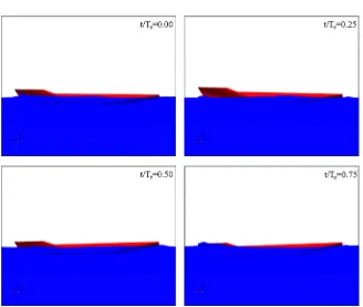
For the purpose of visualisation,Fig. 12displays how the vessel responds to incident head seas in a period of encounter. The pictures are snapshots from the simulation of Case 3 after the solution has stabilised. The corresponding animation for thisfigure is provided in Electronic Annex II.
Supplementary material related to this article can be found online athttp://dx.doi.org/10.1016/j.oceaneng.2015.01.011.
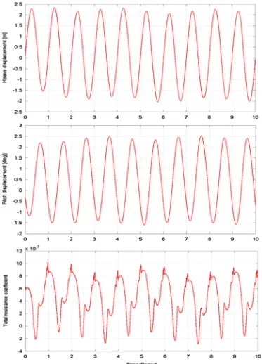
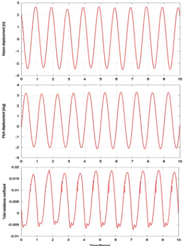
The time histories of heave, pitch andCTthat belong to all the
validation cases, as shown inFigs. 13–15, were recorded over the last ten periods of encounter.
As explained in the previous section, heave, pitch and the drag histories were evaluated by using the Fourier Series expansion. As an example, the FS approximations of the heave, pitch andCTtime
histories in Case 3 covering the last three periods of encounter are
shown inFig. 16. In thefigure, the heave and pitch time histories were evaluated by approximating a second order FS expansion to the raw record, however, for theCTrecords, a FS expansion of a
much higher order (thirty) was approximated to the raw data. From the comparison inFig. 16, it is apparent that the heave and pitch responses of the vessel are well presented by the FS expansion, whereas the FS approximation does not match well with the rawCT
records. This is because in Case 3, the total resistance exhibits highly nonlinear behaviour, due to resonance. However, this should not pose a problem since the zeroth FS harmonics are used inCTcalculations.
The same approach is also used when evaluating experimental time records. Also, it should be borne in mind that in Cases 4 and 6, the total resistance time histories are much closer to linearity (seeFigs. 14 and 15).
5.1.5. Verification study
A verification study was undertaken to assess the simulation numerical uncertainty,USN, and numerical errors,
δ
SN. In the presentwork, it was assumed that the numerical error is composed of iterative convergence error (
δ
I), grid-spacing convergence error (δ
G) andtime-step convergence error (
δ
T), which gives the following expressions forthe simulation numerical error and uncertainty (Stern et al., 2001):
δ
SN¼δ
Iþδ
Gþδ
T ð16ÞU2SN¼U 2 IþU
2 GþU
2
T ð17Þ
whereUI,UGandUTare the uncertainties arising from the iterative,
grid-spacing convergence, and time-step convergence errors, respectively.
The verification study was carried out for the resonant case (Case 3) because, according toWeymouth et al. (2005), large motions and accelerations tend to cause the highest numerical errors. This therefore can be regarded as a‘worst-case test’.
Xing and Stern (2010)state that the Richardson extrapolation method (Richardson, 1910) is the basis for existing quantitative numerical error/uncertainty estimates for time-step convergence and grid-spacing. With this method, the error is expanded in a power series, with integer powers of grid-spacing or time-step
[image:11.595.130.458.456.733.2]Fig. 12.Four snapshots of motions of the vessel and the free surface in a given period of encounter. Table 6
The total resistance and added resistance coefficients in the validation study.
Case no. CTs σaw
3 EFD (Simonsen et al., 2013) 5.133103
9.106
The Current CFD 4.644103
8.128
Error (% of EFD) 9.52 10.74
4 EFD (Simonsen et al., 2013) 5.843103 8.617
The Current CFD 5.481103 8.269
Error (% of EFD) 6.19 4.04
6 EFD (Otzen and Simonsen, 2010) 4.146103
1.916 The Current CFD 3.794103
1.717
taken as afinite sum. Commonly, only thefirst term of the series will be retained, assuming that the solutions lie in the asymptotic range. This practice generates a so-called grid-triplet study.
Roache's (1998)grid convergence index (GCI) is useful for estimat-ing uncertainties arisestimat-ing from grid-spacestimat-ing and time-step errors. Roache's GCI is recommended for use by both the American Society of Mechanical Engineers (ASME) (Celik et al., 2008) and the American Institute of Aeronautics and Astronautics (AIAA) (Cosner et al., 2006).
For estimating iterative errors, the procedure derived byRoy and Blottner (2001)was used. The results obtained from these calculations suggest that the iterative errors for TF3, TF5, andCTare
0.181%, 0.164%, and 0.312% of the solution for thefinest grid and smallest time-step.
[image:12.595.115.488.56.574.2]Grid-spacing and time-step convergence studies were carried out following the correlation factor (CF) and GCI methods ofStern et al. (2006). The convergence studies were performed with triple solutions using systematically refined grid-spacing or time-steps. For example, the grid convergence study was conducted using three calculations in which the grid size was systematically coarsened in all directions whilst keeping all other input parameters (such as time-step) constant. The mesh convergence analysis was carried out with the smallest time-step, whereas the time-step convergence analysis was carried out with thefinest grid size.
To assess the convergence condition, the convergence ratio is used as given in Eq.(18):
Rk¼
ε
k21ε
k32 ð18Þ
In Eq.(18)
ε
k21¼Sk2Sk1andε
k32¼Sk3Sk2are the differencesbetween medium-fine and coarse-medium solutions, where Sk1, Sk2,Sk3correspond to the solutions withfine, medium, and coarse
input parameters, respectively. The subscript k refers to thekth input parameter (i.e. grid-size or time-step) (Stern et al., 2006).
Four typical convergence conditions may be seen: (i) monotonic convergence (0oRko1), (ii) oscillatory convergence (Rko0;|Rk|o1), (iii) monotonic divergence (Rk41), and (iv) oscillatory divergence (Rko0;|Rk|41) (Stern et al., 2006).
For condition (i), the generalised Richardson extrapolation method is used to predict the numerical error and uncertainties. For condition (ii), the uncertainty is predicted by:
Uk¼12ðSUSLÞ ð19Þ
whereSUandSLare the maximum and minimum of the solutions
from the corresponding convergence study. For diverging condi-tions (iii) and (iv), neither error nor uncertainty can be assessed.
For the mesh convergence study, a uniform refinement ratio (rG)
[image:13.595.109.474.56.548.2]was chosen to be√2 which was applied only to the overset region, meaning that the background mesh configuration was not altered. This enabled the incident waves to be modelled efficiently through the computational domain. Without this adjustment, the wave would not have been captured well with a coarser grid configuration, leading to
misleading results. Based on the mesh refinement ratio, thefinal mesh numbers for each mesh configuration are listed inTable 7.
The time-step convergence study was conducted with triple solutions using systematically lessened time-steps based on a uniform refinement ratio (rT) of 2, starting from
Δ
t¼Te/29.The verification parameters of the heave and pitch transfer functions and the total resistance coefficients for the grid spacing and time-step convergence studies are demonstrated inTables 8 and 9, respectively.
In Tables 8 and 9, the corrected simulation value (Sc) is
calculated bySc¼S
δ
nG, where S is the simulation result. Also, Ucis the corrected uncertainty. For more detailed information onhow to calculate these uncertainties, reference can be made to
Stern et al. (2006). The notation style of this reference was used in this study, to enable the verification results to be presented clearly.
As can be seen from the results listed in Tables 8 and 9, reasonably small levels of uncertainty were estimated for the motion transfer functions. On the other hand, relatively large uncertaintiesUG(16.53% and 9.75%) were predicted forCT, using
the CF and GCI methods, respectively. However, these values reduce to 4.37% and 1.95%, respectively, when the corrected uncertainties (UGc) are estimated. This implies that the total drag
force in the resonant case is very sensitive to the grid size resolution. It is expected that the uncertainties for the total resistance coefficient in the other cases are smaller than those in Case 3.
[image:14.595.120.487.54.548.2]As a result of the convergence studies, corrected and uncor-rected verification parameters of the heave and pitch transfer functions and the total resistance coefficients are given inTable 10. In the table, the subscriptcrefers to the corrected parameters.
Stern et al. (2006)specify that in order to determine whether a validation has been successful, the comparison errorE must be compared toUV, the validation uncertainty, given by
U2V¼U 2 DþU
2
SN ð20Þ
whereUDis the uncertainty in experimental data, which is 5.83%
in Simonsen et al.'s EFD data.
Since the absolute value of the comparison errorEis smaller than UV, the heave and pitch transfer functions, as well as the
total resistance coefficient, were validated for both the corrected and uncorrected case. The uncertainty levels were estimated to be 6.12%, 5.84% and 7.07%, respectively, when calculated using the CF method. When the GCI method is used to assess these uncertainties, these values become 5.84%, 5.85% and 6.12%, respectively.
5.2. Calm water results
[image:15.595.113.472.57.556.2]Having validated the CFD model, and having performed the necessary verification study, the reminder of this section addresses the mainfindings of this work.
Fig. 16.FS approximation of the heave, pitch and total resistance time histories for the last 3 periods of encounter, Case 3.
Table 7
Thefinal cell numbers for each mesh configuration as a result of the mesh convergence study.
Mesh configuration Cell number (N)
Background Overset Total
Fine 3,572,074 6,357,286 9,929,360
Medium 3,572,074 3,143,679 6,715,753
[image:15.595.302.553.614.683.2]The calm water total resistance coefficients (CT), the dynamic
sinkage results non-dimensionalised with the ship length (x30/LBP)
[image:16.595.42.563.82.148.2]and the trim angle (x50) in degrees are presented for two speeds in
Table 11. The CFD results contained inTable 11for 24 knots are under predicted by approximately 6.7% compared to the towing tank results ofSimonsen et al. (2013). The estimation of the full scaleCTvalue at 24
knots through the towing tank tests was explained in the previous sub-section. Unfortunately, experimental results for this ship operating at a speed of 19 knots are not available in the literature, and thus could not be included in this paper. The quantities listed in the table decrease as the ship speed is reduced to 19 knots, as expected.
5.3. Ship motion responses in head seas
The results obtained using the proposed RANS method were compared to those obtained using the potential theory-based fre-quency domain code VERES. In the potential theory the fluid is assumed to be homogeneous, non-viscous, irrotational and incom-pressible. The method used to calculate ship motions in VERES is based on the two-dimensional, linear, strip theory formulation by
Salvesen et al. (1970). For more information about this seakeeping
code, reference can be made to the theory manual of the software (Fathi and Hoff, 2013).
Heave and pitch transfer functions predicted by CFD, EFD and VERES at the two different speeds, listed inTable 12, are illustrated graphically inFigs. 17 and 18. This gives a clearer depiction of the responses of the vessel to head waves, enabling a more facile comparison among the different approaches. The comparison errors are also listed in Table 12. The EFD data are taken from
Simonsen et al. (2013).
As clearly seen fromFig. 17andTable 12, compared to the EFD, the motions are generally better predicted by the CFD method than by the potential theory-based software package, particularly for heave motion. When Figs. 17 and 18are compared with each other, the discrepancies between the CFD and VERES are much more pro-nounced at 24 knots. Generally, VERES seems to overpredict the motions compared to the CFD method, particularly at 19 knots. Additionally, as can be understood fromTable 12, the heave and pitch responses of the vessel tend to decrease at 19 knots, compared to those at 24 knots. However, it is predicted that although the vessel decreases its speed when operating in head seas where
λ
/L¼1.0, the heave and pitch responses increase at 19 knots (in Case 8). This is due to the fact that the encounter frequency in that wave condition becomes close to the natural heave and pitch frequency as the speed is reduced to 19 knots.5.4. Resistance coefficients
The resultant added resistance and total resistance coefficients of the vessel in question using the different methods are tabulated in
Table 13. Also, the comparison errors which are based on EFD data are listed in the table. Since the experimentalCTvalues are not available,
only the results from CFD and potential theory calculations are given for the total resistance coefficients in the table. In addition, the added resistance coefficients at both ship speeds are shown graphically in
Fig. 19.
For the added resistance calculations, the employed potential theory-based software uses the method of Gerritsma and Beukelman (1972), which is based on the determination of the energy of the radiating waves and a strip-theory approximation (Fathi and Hoff, 2013).
As Table 13 and Fig. 19 jointly show, for the added resistance coefficients, CFD agrees much better with the experiments when compared to VERES for the ship speed of 24 knots. Both methods underpredict the added resistance coefficients compared to the EFD data. When the added resistance predictions at the two speeds are compared, it is obvious that the discrepancies between VERES and CFD
Table 8
Grid convergence study for TF3, TF5, andCT.
Para-meter rG Solutions RG δnG(%S1) UG(%S1) UGc(%S1) Sc EFD
S1 S2 S3 CF GCI CF GCI
TF3 √2 0.946 0.918 0.814 0.270 2.964 4.83 1.37 1.87 0.27 0.974 0.950
TF5 √2 0.664 0.678 0.708 0.489 2.154 2.31 2.58 0.22 0.52 0.650 0.693
[image:16.595.43.563.187.254.2]CT √2 4.644103 4.485103 4.255103 0.695 3.430 16.53 9.75 4.37 1.95 4.803 103 5.133103
Table 9
Time step convergence study for TF3, TF5, andCT.
Para-meter rT Solutions RT δnT(%S1) UT(%S1) UTc(%S1) Sc EFD
S1 S2 S3 CF GCI CF GCI
TF3 2 0.946 0.925 0.846 0.259 0.724 0.85 0.95 0.09 0.20 0.953 0.950
TF5 2 0.664 0.646 0.578 0.274 0.927 1.28 1.31 0.14 0.26 0.670 0.693
[image:16.595.43.293.291.386.2]CT 2 4.644103 4.382103 3.504103 0.298 1.880 3.44 3.00 0.51 0.60 4.731103 5.133103
Table 10
Validation of heave and pitch transfer functions and total resistance coefficient.
Para-meter USN(%EFD) UD UV(%EFD) E(%)
CF GCI CF GCI
TF3 4.89 1.70 5.83 7.61 6.07 0.42
TF3c 1.87 0.38 5.83 6.12 5.84 3.07
TF5 2.52 2.51 5.83 6.35 6.35 4.18
TF5c 0.33 0.53 5.83 5.84 5.85 5.52
CT 15.02 9.24 5.83 16.11 10.92 9.52
[image:16.595.43.294.434.497.2]CTc 4.00 1.87 5.83 7.07 6.12 5.01
Table 11 Calm water results.
Speed (kn) CT x30/LBP x50(deg)
24 EFD (Simonsen et al., 2013) 0.002414 0.0021 0.1853
CFD 0.0022945 0.00196 0.1775
Error (% of EFD) 4.95 6.67 4.21
are much more pronounced at 24 knots, in a similar manner to the ship motion predictions. This is expected, because the results obtained from the linear potential theory are more accurate at moderate speeds than at higher speeds.
5.5. Increases in the effective power of the vessel due to added resistance
The effective power (PE) is the power required to propel the
vessel forward through the water at a constant speed, and is thus
[image:17.595.31.555.75.418.2]calculated as the product of the speed and the total resistance. The effective power can be computed using CFD approaches such as the one which is demonstrated in this paper, however this is not the case for the fuel consumption. This is due to the very complex interplay of the variables that contribute to fuel consumption, such as engine load, SFOC (Specific Fuel Oil Consumption), propeller speeds and many others, which depend on a vessel's specifics at different operating conditions. Therefore, in this paper, the fuel consumption will not be calculated directly. Instead, the percen-tage increase in effective power due to the added resistance in
Table 12
The transfer functions for all cases by three different methods (Error (E) is based on EFD data).
Case no. Ship speed (kn) Froude number TF3 TF5
CFD EFD VERES CFD EFD VERES
C U Fn Result E(%) Result E(%) Result E(%) Result E(%)
1 24 0.260 Calm water Calm water
2 0.738 1.35 0.749 0.580 22.46 0.542 0.64 0.539 0.544 1.02
3 0.946 0.42 0.950 1.005 5.74 0.664 4.18 0.693 0.777 12.12
4 1.003 9.39 1.107 1.098 0.79 0.895 7.83 0.971 0.914 5.84
5 0.899 4.82 0.945 1.061 12.25 0.985 7.32 1.063 0.976 8.18
6 0.847 5.99 0.901 0.992 10.15 1.085 4.63 1.037 1.043 0.55
7 19 0.206 Calm water Calm water
8 0.754 – – 0.646 – 0.550 – – 0.598 –
9 0.846 – – 0.852 – 0.662 – – 0.778 –
10 0.856 – – 0.885 – 0.802 – – 0.894 –
11 0.858 – – 0.887 – 0.874 – – 0.952 –
12 0.878 – – 0.910 – 1.007 – – 1.023 –
[image:17.595.38.552.79.249.2]Fig. 17.A comparison of the ship motions using different methods at a speed of 24 knots (the left and right-hand sides of the graph show heave and pitch TFs, respectively).
[image:17.595.43.547.474.608.2]