Comparing placentas from normal
and abnormal pregnancies
Alex Heazell∗ Simon Cotter Laura Gallimore
David Greenhalgh Stuart Kennedy Vaclav Klika Maur´ıcio Kritz Poul Nielsen Katharine Preedy Ida Pu
Ani Setchi Jennifer Siggers Robert Whittaker†
Mathematics-in-Medicine Study Group University of Strathclyde
September 2010
Abstract
This report describes work carried out at a Mathematics-in-Medicine Study Group. It is believed that placenta shape villous network char-acteristics are strongly linked to the placenta’s efficiency, and hence to pregnancy outcome. We were asked to consider mathematical ways to describe the shape and other characteristics of a placenta, as well as forming mathematical models for placenta development.
In this report we propose a number of possible measure of placen-tal shape, form, and efficiency, which can be computed from images already obtained. We also consider various models for the early devel-opment of placentas and the growth of the villous tree.
∗
Problem presenter. †Report editor.
1
Report on a problem studied at the UK Mathematics-in-Medicine Study Group Strathclyde 2010
CONTENTS 2
Contents
I Introduction 4
1 Background 4
2 Description of the placenta and its development 5
3 Study group aims and objectives 8
II Quantifying Placental Properties 10
4 Image data and processing 10
5 Placenta quantification using moments 13
5.1 Cord insertion point . . . 13
5.2 Circularity of placental shape . . . 14
5.3 Ellipticity of placental shape . . . 15
5.4 Summary of proposed measures . . . 17
6 Placental shape from rule and compass 18 6.1 The shape-observation problem . . . 18
6.2 Shape inspectors . . . 18
6.3 About placental shapes and measures . . . 22
7 Index of efficiency for the vascular network 24 7.1 Introduction . . . 24
7.2 Defining the index . . . 24
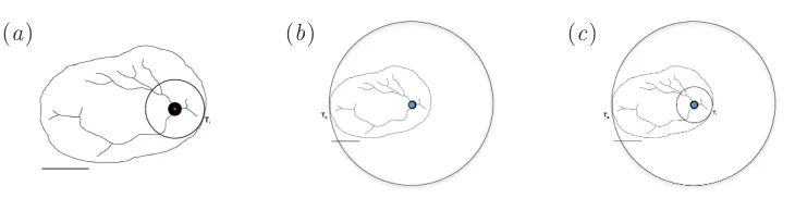
7.3 CalculatingE from photographs . . . 25
7.4 Results . . . 26
7.5 Discussion . . . 26
III Mathematical Modelling 29 8 Mechanical model of the blood flow 29 8.1 Introduction . . . 29
8.2 Porous medium model of blood flow in the placenta . . . 29
8.3 Network model of the large vessels . . . 34
CONTENTS 3
8.5 Discussion . . . 36
9 Development of the villous tree 39
9.1 Modelling the villi growth rate as linearly dependent on nu-trients . . . 39 9.2 Modelling the development of the villi using chemotaxis and
diffusion . . . 41
10 Early Placental development model 47
10.1 Model description . . . 47 10.2 Simulation results . . . 49 10.3 Conclusions . . . 51
11 Formation of vascular trees 52
11.1 Problem description . . . 52 11.2 Model of growth . . . 53 11.3 Outline of algorithm . . . 53
IV Conclusions and Future Work 55
12 Conclusions and future work 55
V Appendices 57
A Matlab code 57
B Proofs for β and γ 59
C R code for the efficiency index 62
4
Part I
Introduction
1
Background
A healthy placenta is essential for a healthy outcome of pregnancy. At term, the human placenta is described as a discoid organ approximately 20–25 cm in diameter and 3 cm thick. The umbilical cord usually inserts in the centre of the placenta. The human placenta consists of a villous tree which is bathed in maternal blood. The villous tree contains fetal vessels, carrying fetal blood into terminal villi where it is brought into close proximity with maternal blood to optimise the transfer of nutrients and oxygen from mother to fetus and waste products in the opposite direction. As a result the function of the human placenta is very closely related to its structure.
2 DESCRIPTION OF THE PLACENTA AND ITS DEVELOPMENT 5
The link between placental shape and poor pregnancy outcome is un-certain. What is certain is that placental shape is determined by events in early pregnancy. Immediately after implantation the embryo is spherical and is fully embedded in maternal tissue (decidua). Initially the placenta is formed from primary villi which undergo a series of branches. Over the early weeks of pregnancy, these villi branch and cells invade from the villi to convert the maternal uterine arteries that supply the developing fetus. The placental villi become vascularised with vessels growing from placental villi and towards blood vessels growing out from the base of the umbilical cord. When maternal blood supply starts, the placenta regresses from a sphere to a disc, if the maternal blood supply is abnormal this regression is uneven and irregular which will result in an abnormal placental shape and a non-central cord. Modelling the growth of the placental shape and the branching network of fetal vessels, may allow understanding of the factors that drive the development of placental shape, which cannot be viewed in real-time in human placental development.
2
Description of the placenta and its development
The human placenta consists of a villous tree which is bathed in maternal blood. The villous tree contains fetal vessels, carrying fetal blood into ter-minal villi where it is brought into close proximity with maternal blood to optimise the transfer of nutrients and oxygen from mother to fetus and waste products in the opposite direction. The function of the human placenta is very closely related to its structure.
The placenta is primarily a trade site for exchange of nutrients between maternal and fetal blood. It “provides anchorage, establishes a fetal vascular network in association with maternal blood supply but without connection” as well as hormonal support (Stewart, 2009). It acts as an endocrine gland with many physiological functions, such as immune protection. It has a large surface area which increases as the fetus grows.
The outer surface of the uterus is a glandular tissue called the epithelium. The endometrial stroma lies beneath this and is the tissue lining the uterus. Together, the glandular lining and the endometrial stroma are referred to as the endometrium of the uterus.
2 DESCRIPTION OF THE PLACENTA AND ITS DEVELOPMENT 6
Then the epithelium is penetrated. Next follows an invasive phase when the endometrial stroma is penetrated. Then a reaction of the stromal cells follows. This is particularly marked in primates and rodents. The next thing that happens is interstitial implantation in which the blastocyte lies within the substance of the endometrium.
The histiotrophic phase is next. Histiotroph is an extracellular material derived from the endometrium and the uterine gland that accumulates in the space between the maternal and fetal tissues. This mechanism transfers nutrients from the mother to her fetus. This histiotrophic stage is short in humans. The haemotrophic phase follows. Haemotrophic nutrition is the ex-change of blood-borne nutrients between the maternal and fetal circulations (Burtonet al., 2002).
Uterine glands provide histiopathic nutrition for the human fetus during the first trimester of pregnancy (Stewart, 2009). The developing embryo ini-tially receives nutrients from milk-like secretions of the uterine tube. In the histiopathic phase it receives nutrition from the breakdown of tissues such as glands and stroma around the site of implantation. In the haemotrophic phase the embryo, and later fetus, receives nutrition from blood.
Figure 1 identifies some of the key stages in the development of the fetus. At timet= 0 the sperm reaches the egg and fertilises it. Within a couple of days the embryo leaves the Fallopian tube, reaches the uterus and embeds itself into the decidua of the uterine wall, where it receives nutrients from the maternal spiral arteries. There, it starts differentiating into a spherical structure. The placenta begins to develop upon implantation on one side of the sphere.
There are several hypotheses about how the villous tree develops based on the fact that it is hard to differentiate between different villi before they have been vascularised. One hypothesis is that villi grow one at a time with the extra one added only when the embryo becomes big enough to reach the next spiral artery. Another hypothesis is that initially there are 40–60 ‘roots’ that develop simultaneously using the nutrient from the neighbouring spiral arteries but in the end the growing pattern is such that all villi are opposite a spiral artery. The first hypothesis is generally better accepted due to the fact that the width of a healthy placenta is relatively uniform and the size of each villa is very similar, meaning the villi tend to grow sideways rather than in all directions.
2 DESCRIPTION OF THE PLACENTA AND ITS DEVELOPMENT 7
Figure 1: Key stages in the development of an embryo. Photographs by Lennart Nilsson.
[image:7.595.215.396.446.622.2]3 STUDY GROUP AIMS AND OBJECTIVES 8
[image:8.595.127.486.129.275.2](a) (b)
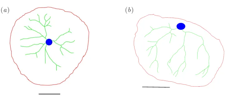
Figure 3: Photographs of placentas: (a) A normal healthy placenta, and (b) a placenta with a lateral cord insertion point.
and to reduce the nutrients being delivered by the maternal blood. It is believed that the villi continue to grow due to nutrients such as fats and sugars present in the uterine wall or the nutrients delivered by the spiral arteries away from the villi.
Until timet= 7 ort= 8 weeks the embryo is not physically connected to the villi. Around that time the umbilical cord that grows from the embryo reaches the placenta. The details surrounding this process are not known. One hypothesis is that the umbilical cord attaches itself to the place where the embryo first embedded itself into the uterine wall; another is that there are some factors that tell the embryo where the nutritional centre of mass of the placenta is.
In any case, fetal blood starts to perfuse the placenta and by timet= 10 weeks the villous tree has developed the maximum number of villi, is fully vascularised, the maternal spiral arteries have opened up and are feeding nutrients for both the embryo and placenta to grow (figure 2). By time t= 40 weeks the size of the placenta is around 20×20×3 cm3 and all the villi are lined up to be opposite some spiral artery.
3
Study group aims and objectives
In this project workshop we were specifically interested in developing models of:
3 STUDY GROUP AIMS AND OBJECTIVES 9
Figure 4: A photograph of a bipartite placenta.
structure).
2. By modelling the normal development of blood vessels, can inferences be made about the abnormal patterns seen in complicated pregnancies.
Using the expected models of placental development can valid measures be made to enable the comparison of:
1. The circularity of the placenta
2. The centrality of the umbilical cord insertion
3. The network of vessels on the fetal surface of the placenta
in normal and abnormal pregnancies.
10
Part II
Quantifying Placental Properties
We would like to clarify the link between placental shape and pregnancy outcome. In order to investigate this, we need to be able to objectively quantify key features of the placenta. Some of the key placental attributes highlighted by clinicians as being of interest include; size of the placenta, how centrally the umbilical cord is inserted and whether the placenta has a regular, circular shape.
The problem of correlating constitutive or functional behaviour of ob-jects with their shape is not new. In 1966, Marc Kac published a paper entitledCan one hear the shape of a drum?, where he pointed out that con-cerns such as this goes back at least to the beginning of last century (Kac, 1966). The question posed by Mark Kac relates to comparing eigenvalues of the Laplacian operator with different domains (shapes) and have been answered in the negative by Gordonet al. (1992) for non-convex domains.
The ‘functionality’ of a drum is much simpler than that of placentas and the referred work shows that the problem is not easy. However, placentas are more convex than not. Moreover, we are considering placenta shapes from a visual stand and concerned also with the coverage of the baby’s vas-cular network. Despite the differences, the analysis of the hearing problem provides hints about possible measures and measuring procedures.
There are many possibilities for quantifying placental shape. Yampolsky
et al. (2008) describe measuring an average placental radius based on an equally spaced template having 20 sectors of 18◦. The methods described here generalise their measures both with respect to where and to what to measure and take into account more of the available information.
4
Image data and processing
4 IMAGE DATA AND PROCESSING 11
[image:11.595.125.489.119.274.2](a) (b)
Figure 5: Manually drawn traces of the two placentas in figure 3. The outline is shown in red, major vessels in green, the site of cord insertion in blue, and the scale bar in black. The placenta in (a) is normal, while that in (b) has a lateral cord insertion point.
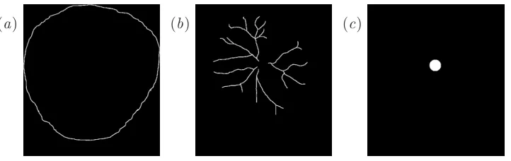
These outlines had been traced from photographs, manually in a computer drawing package. In order to distinguish easily the different structures, the placental outline was coloured red, the site of the cord insertion was coloured blue and the main arterial network was coloured green, whilst the scale bar was coloured black as shown in figure 5. The outline images were stored as tiff files.
The Matlab code to read in these images can be found in Appendix A. The files are read into Matlab as three-dimensional matrix. For example if the image is 200×300 pixels, Matlab reads this as a 200×300×4 array, which can be thought of as four 200×300 pixel images stacked on top of each other. The first layer contains red values, the second green values and the third blue values, so these correspond to the placenta, vessel and cord outlines respectively. Each pixel has a number between 0 and 1, where 0 corresponds to the black background and 1 corresponds to the maximum intensity of that layer’s colour. The fourth layer picks out all the outlines and the scale bar, so the scale bar can be isolated by subtracting off the other three images. In order to obtain binary images, the images are thresholded, so any pixel value below 0.5 is set to 0 and any pixel value above 0.5 is set to 1. The isolated features corresponding to the colour image in figure 5(a) are shown in figure 7.
4 IMAGE DATA AND PROCESSING 12
(a) (b) (c)
[image:12.595.134.473.124.304.2](d) (e)
Figure 6: Further traces of typical placentas shapes, showing the major vessels and cord insertion point. (a), (b) and (c) are RFM placentas, (d) and (e) are normal placentas. Observe that placentas (c) and (d) have a similar exterior shape, but quite different different vascular tree structures.
(a) (b) (c)
Figure 7: Features extracted by Matlab from the colour image in fig-ure 5(a): (a) the edge of the placenta, (b) the major vessels, and (c) the cord insertion point.
[image:12.595.128.489.375.489.2]5 PLACENTA QUANTIFICATION USING MOMENTS 13
5
Placental shape and cord insertion point using
moments
5.1 Cord insertion point
We would like quantify how central the site of cord insertion is, i.e. how far away the insertion point is from a ‘central’ point in the placenta. We define this central point as the centre of mass ¯xof the placenta, given by
¯
x= 1
A
ZZ
xdA , (5.1)
where
A=
ZZ
dA . (5.2)
is the total area, and x= (x, y) is the position vector of each point inside the placenta.
These integrals over the placenta area can be approximated by summing over the pixels in the image, multiplying the mean value of the integrand in each square pixel by its aread2p. Since the mask Mij takes the value 0 for
pixels outside the placenta, and 1 for points inside, we can multiply byMij
and then sum over all pixels to pick out the ones we require. It is convenient to introduce
N =X
i,j
Mij, (5.3)
as the total number of pixels within the placenta area. The integrals for ¯x
andA can then be approximated by
¯
x≃ 1
N
X
i,j
Mij(xij, yij), (5.4)
A≃d2pN (5.5)
where (xij, yij) are coordinates of the centre of the (i, j)th pixel.
Since the cord is defined in the image by a region rather than a point, we use the same technique to calculate the centre of mass of the cord region, denoting thisxcord.
Having calculated A, ¯x and xcord, we define our measure α of the cen-trality of the cord by
α= |xpcord−x¯|
5 PLACENTA QUANTIFICATION USING MOMENTS 14
This is the distance between centres of the cord and the placenta, normalised by the radius of the circle with the same area as the placenta. This normali-sation ensures that our measure of cord centrality is not affected by the size of the placenta. We note that α >0 and that α is zero if and only if the centre of the cord and the centre of the placenta coincide.
5.2 Circularity of placental shape
In order to consider measures of the shape of the placenta, we first introduce some notation,
σ2xx= 1 A
ZZ
|x−x¯|2dA, (5.7)
σ2yy= 1 A
ZZ
|y−y¯|2dA. (5.8)
Bothσxx2 andσ2yy are variances which describe how spread out points in the placenta are from its centre of mass. We calculate the discrete approxima-tions,
σxx2 ≃ 1 N
X
ij
Mij x2ij −x¯2
, (5.9)
σxx2 ≃ 1 N
X
ij
Mij y2ij−y¯2
, (5.10)
We defineσ2 =σ2
xx+σ2yy. We show in Appendix B that, for a given area,
the shape which minimisesσ2 is a circle. The corresponding minimal value is found to be
σ2circle= 1 A
ZZ
x2+y2dA= 2π A
Z √A/π
0
r3dr = A
2π. (5.11)
In order to obtain a measure of how far the placenta is from circular, we consider how muchσ2 varies fromσ2circle. We define
β = σ2 σ2 circle −1
1/2
=
2πσ2
A −1
1/2
. (5.12)
5 PLACENTA QUANTIFICATION USING MOMENTS 15
measure is linear in small deformations from a circle, and so better captures small deformations.
A similar calculation to (5.11), shows that for an ellipse with major axis length aand minor axis lengthb,
σellipse2 = a 2+b2
4 , ⇒ β =
a2+b2 2ab −1
1/2
, (5.13)
so ifa= 2b, then β= 1/2.
5.3 Ellipticity of placental shape
Largeβvalues, indicate poor circularity, but they fail to distinguish between two key classes of shape — the placenta could either be a regular oval shape, with a smooth edge, or a very irregular, possibly lobed shape without a direction in which it is elongated. We would therefore like to obtain one or more additional measures that describe how elliptical a given placenta shape is.
To do this, we consider the covariance matrix,
C=
σxx2 σ2xy σ2
xy σyy2
, (5.14)
whereσ2
xx and σyy2 are as defined above, and
σxy2 = 1 A
ZZ
(x−x¯)(y−y¯) dA≃ 1 N
X
Mij(xiyi−x¯y¯). (5.15)
SinceCis a real symmetric matrix, it has a complete set (two in this case) of orthogonal eigenvectors. The two eigenvectors define the two principal directions for the shape. The sizes of the eigenvectors give the degrees of elongation or compression in these two directions. If the placenta has an axis about which it is elongated, then the eigenvector corresponding to the larger of the the two eigenvalues, points along this axis. We select σa2 to be the larger of the two eigenvalues and σ2b the smaller. The ratio of the eigenvalues
λ= σa σb ≥
1, (5.16)
5 PLACENTA QUANTIFICATION USING MOMENTS 16
[image:16.595.120.489.129.272.2](a) (b)
Figure 8: Outlines of two example placentas, with the cord insertion points shown. (a) A reasonably circular placenta, with α = 0.0756, β = 0.0802, γ = 0.0724 and λ = 1.05. (b) A more irregular and less circular placenta, which hasα= 0.237,β = 0.268, γ= 0.136 andλ= 1.38.
Analogously toβ, we would like to consider how much the placenta varies from the best-fitting ellipse. We define this ellipse to have the same areaA and aspect ratioλ as the placenta. So if the ellipse has semi-axesa and b, we require
A=πab , σa σb
= a
b, (5.17)
which implies
a=
Aσa
πσb
1/2
, b=
Aσb
πσa
1/2
. (5.18)
Substituting fora andb in Equation (5.13) we see
σ2ellipse= A 4π
σ2
a+σ2b
σaσb
= Aσ
2
4πσaσb
, (5.19)
(The second equality results from the fact thatσ2 =σ2
a+σ2b, as the sum of
the eigenvalues of a matrix is equal to its trace.)
Our corresponding measure of departure from an ellipse is therefore given by
γ = σ
2
σ2 ellipse
−1
!1/2
=
4πσaσb
A −1
1/2
. (5.20)
5 PLACENTA QUANTIFICATION USING MOMENTS 17
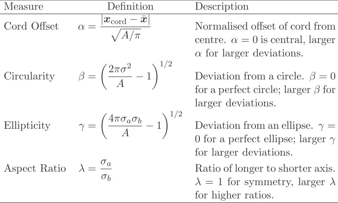
Measure Definition Description
Cord Offset α= |xpcord−x¯|
A/π Normalised offset of cord fromcentre. α= 0 is central, larger
α for larger deviations.
Circularity β =
2πσ2
A −1
1/2
Deviation from a circle. β = 0 for a perfect circle; largerβfor larger deviations.
Ellipticity γ =
4πσaσb
A −1
1/2
Deviation from an ellipse. γ = 0 for a perfect ellipse; largerγ for larger deviations.
Aspect Ratio λ= σa σb
[image:17.595.128.468.130.335.2]Ratio of longer to shorter axis. λ= 1 for symmetry, larger λ for higher ratios.
Table 1: A summary of the four measures proposed in§5.
5.4 Summary of proposed measures
In this section, we have proposed four measures α, β,γ, andλto quantify the centralness of of the cord insertion point and the shape of the placenta. A summary of these measures, is given in table 1, and two example placenta are shown in figure 8, along with the values of the measures.
6 PLACENTAL SHAPE FROM RULE AND COMPASS 18
6
Placental shape from rule and compass
6.1 The shape-observation problem
We are interested not only in the geometry of the border of the placenta but also in the localization of the allantois with respect to this border. Furthermore, it would be nice to identify whatever allows for distinguishing normal pregnancy placentas from reduced fetal movement (RFM) placentas (see figure 6).
It is quite clear that we can momentarily disregard the thickness and the shell-like form of their ‘superior’ face, together with its curvature, and con-sider placentas as 2-dimensional geometric forms. Moreover, each placenta is a single piece whatever the pregnancy and its shape is connected.
Hence, let Ω ⊂R2 be a simply connected domain in the plane and∂Ω its boundary. Denoting the closure of Ω by Ω• and its interior by Ω◦, we have that:
∂Ω = Ω•\Ω◦. (6.1)
The border∂Ω of Ω is usually a 1-dimensional continuous variety (a line), not necessarily differentiable nor convex. It is, nevertheless, closed and without extremities dividingR2 into two disjoint regions.
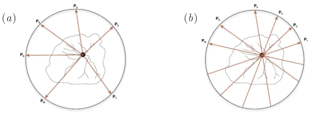
6.2 Shape inspectors
To inspect the shape of Ω, or of∂Ω, let us consider measurement templates formed by a finite collection of points: one interior to Ω, P ∈ Ω◦, and
N other points Pi ∈ R2 \Ω•, ∀i ∈ {1, . . . , N}, exterior to it. Without loss of generality, the exterior points can be taken on a circle encompassing Ω (see figure 9). Based on these templates, some geometrical constructs and measures will be developed for inspecting 2D-shapes. These templates are nevertheless not fixed. Both the points and the number of points may vary during an inspection procedure. Hence, the templates may be taken as parameters for the measures. The set of rays defined in equation (6.2) will be denoted by πr and the set of lines defined in equation (6.3) by πl. It is expected that the simple mathematical objects here described will
contribute to establish data collection procedures to enlarge data about placentas consistently and coherently.
We have that P6∈∂Ω andPi6∈∂Ω,∀i= 1, . . . , N. Let
1. the rays starting atP and extending in the direction ofPi which are
parametrically described as: −−→
6 PLACENTAL SHAPE FROM RULE AND COMPASS 19
[image:19.595.149.459.130.245.2](a) (b)
Figure 9: Measuring Templates: (a) rays and (b) lines.
2. and the lines passing throughPand eachPi which are parametrically
described as:
PPi(λ) =P+λ(Pi−P) = (1−λ)P+λPi, λ∈R. (6.3)
Then PPi(0) = Pand PPi(1) =Pi,∀i= 1, . . . , N. In the case of placenta
shapes the point P will generally coincide with the allantois, as suggested in figure 9, but not necessarily.
Furthermore, since ∂Ω is closed and Pand Pi are ‘inside’ and ‘outside’
∂Ω, respectively, the rays−−→PPi(λ) intersect∂Ω at least in one point and the
linesPPi(λ) at least in two points. Let
∂rΩi =∂Ω∩ {PP−−→i(λ), λ >0} (6.4)
and
∂lΩi=∂Ω∩ {PPi(λ), λ∈R}. (6.5)
If #(A) denotes the cardinality of a setA, we have that:
Lemma 6.1. If Ω is bounded, #(∂rΩi) is odd and #(∂lΩi) is even.
Proof. Trivial. (R2 is a Haursdorf space and ∂Ω divides R2 in two non-intersecting regions)
By introducing the notation,∂l+Ωi =∂Ω∩{PPi(λ)|λ >0}and∂l−Ωi =
∂Ω∩ {PPi(λ)|λ <0}, the set of intersection points between lines and∂Ω
can be described as:
∂lΩi =∂l+Ωi∪∂l−Ωi, (6.6)
where the sets∂l+Ωi and∂l−Ωiare analogous to∂rΩi and both #(∂l+Ωi) and
6 PLACENTAL SHAPE FROM RULE AND COMPASS 20
Definition 6.1. A setSis convex if and only if given a finite set{u1, . . . , up}
in S, all barycentric combinations of{u1, . . . , up} also belong to S, that is, p
X
i=1
λiui ∈S, (6.7)
where 0≤λi ≤1,∀1≤i≤p and p X
i=1
λi= 1. (6.8)
It is clear that one can consider p = 2 without loss of any sort, partic-ularly when S ⊂ R2. (Usually p is chosen to be equal to the dimension of S to simplify convexity tests.) Convexity can be relaxed in many situations by considering star-shaped domains. More information about mathematical properties of convex domains and their algebra can be found in (Rockafellar, 1970, Parts I–III) and (Rockafellar & Wets, 1998, Chap. 2 and 3).
Definition 6.2(Star-shapedness). A setS ⊂R2 is star-shapedif and only if there exists a pointc∈S such that for any other pointP∈S the segment
cP⊂S.
We say that S is star-shaped with respect to the central point c. The central pointcis not unique in general. The set of all possible central points of a star-shaped domainS is a convex set and is called the convex-kernel of S Smith (1968). In the sequel, Bρ(P) will denote a ball of radiusρ centred
at P.
Lemma 6.2. Let Ω be bounded and ∂lΩi be given by equation 6.5. If
#(∂lΩi) = 2, for any P ∈ Ω◦ and P0 ∈ R2\ Ω•, then Ω is star-shaped
if Pis held fixed inside Ωand convex if the P varies throughout Ω◦.
Proof. Whenever #(∂lΩi) = 2, we have that ∂lΩi = {q,Q}. Let us first
introduce some useful notation. Given a pair of points{q,Q}, we define
[q,Q] ={ηq+ (1−η)Q, η∈[0,1]} (6.9)
and
(q,Q) ={ηq+ (1−η)Q, η∈(0,1)} (6.10) to be respectively the closed and open segments connecting the pointsqand
6 PLACENTAL SHAPE FROM RULE AND COMPASS 21
The proof proceeds as follows. Since Ω is bounded, there is a large enough ρ0 such that Ω• ⊂ Bρ0(P). For any point P
′ ∈ Ω◦,P′ 6= P, let P0 =∂Bρ0(P)∩
−−→
PP′. We have that bothP and P′ belong to the segment (q,Q) and thus the segment [P,P′] belongs to Ω◦. Therefore, Ω is star-shaped with respect to the central pointP.
LettingPvary inside Ω, the above reasoning shows that [P,P′]⊂Ω for allP,P′ ∈Ω. Therefore, Ω is convex.
The placenta traces in figure 6 look like being either convex or star-shaped at the given resolution.
Towardsmeasuring forms, let’s begin considering the following values:
dri =minq∈∂rΩid(P,q), (6.11)
for the rays, and
dli = min(δi−, δ+i ),
Dli = max(δi−, δi+), (6.12)
where
δ−i = min q∈∂−l Ωi
d(P,q), (6.13)
δ+i = min q∈∂+lΩi
d(P,q). (6.14)
Note that if #(∂rΩi) = 1, then dri =d(P,q), since ∂rΩi ={q}. Likewise, if
#(∂lΩi) = 2, then
δi− = d(P,q−),
δi+ = d(P,q+); (6.15)
where∂l−Ωi ={q−}and ∂l+Ωi ={q+}.
The following measures associated with Ω and the templates πr and πl
may be defined and are straightforward to evaluate:
E1(Ω, πr) =
N
max
k=1(d
r
i)/
N
min
k=1(d
r
i), (6.16)
E2(Ω, πl) =maxN
k=1(D
l
i/dli), (6.17)
E2′(Ω, πl) =minN
k=1(d
l
i/Dli), (6.18)
E3(Ω, πl) =
N
max
k=1(D
l
i)/
N
min
k=1(d
l
6 PLACENTAL SHAPE FROM RULE AND COMPASS 22
[image:22.595.125.490.123.214.2](a) (b) (c)
Figure 10: Encircling a placenta from inside and outside: (a) from inside, (b) from outside and (c) both.
E3′(Ω, πl) =minN
k=1(D
l
i)/maxNk=1(dli), (6.20)
E4(Ω, πl) =
N
max
k=1(D
l
i+dli)/
N
min
k=1(D
l
i+dli). (6.21)
To define the next measure, let
BR(P,Ω) = \
ρ>0
Bρ(P) such that Ω⊂Bρ(P), (6.22)
and
Br(P,Ω) = [
ρ>0
Bρ(P) such that Bρ(P)⊂Ω. (6.23)
That is,BR(P,Ω) is thesmallest ball centred atPcontaining Ω andBr(P,Ω)
is thelargest ball centred at Pand contained in Ω (see figure 10). Then,
E5(Ω,P) =R/r. (6.24)
The measureE5 and the exterior and interior tangent pointsTe andTi
are not as straightforward to obtain as the previous ones. The finding of BR(P) andBr(P) require a limiting process that must be approximated.
6.3 About placental shapes and measures
The following comments about placental shapes and the measures proposed above are intended as guidelines and navigation lights in gathering data and in the further exploration of any relationship between placental conformation and function. First, comments about the shape.
6 PLACENTAL SHAPE FROM RULE AND COMPASS 23
should be the most efficient possible, we should preferably be considering star-shaped placentas rather than almost circular ones. If the baby’s vessels had no dimension at all, a star-shaped placenta would permit that each of its points be reached by a straight vase, shortening the time the blood needs to flow back and forth.
Of course they are not dimensionless. The effective branching network allows for conforming a shortest path reach with the limited number of branches that may growth from any convergence point. The ability to branch at any point in any direction would require convexity (see Lemma 6.2). How-ever, the finiteness of the branching could easily fill a star-shaped area. From another stand, the irregularities presented by placentas at their borders may conform to star-shaped constrains.
Moreover, we need to remind us that while operational the placenta does have a curvature and is not planar. We should take this into account while measuring and design correcting procedures for the measurements.
Second, we highlight some characteristics of the measures proposed.
E1(Ω, π
r) is a measure of circularity. The larger the number of external
points Pi and the close the measure is to 1, the greater the chances
that the domain be circular.
However, star-shaped domains with regular variations at the border or with variations nearby thePi may trapE1-measurements into giving the impression of circularity.
The measure E2(Ω, π
l) indicates whether there is a radial symmetry
aroundP.
For shapes in the form of ellipses, R is the longer axis while r is the
shortest. Besides that, the lines PTe and PTi are collinear to the
ellipse’s axis. The measure E5 and the exterior and interior tangent points Te and Ti in figure 10 provide indications about eccentricity
and aspect ratio if Ω is close to an ellipsoid.
7 INDEX OF EFFICIENCY FOR THE VASCULAR NETWORK 24
7
Index of efficiency for the vascular network
7.1 Introduction
It is expensive and time consuming to obtain three-dimensional images of human placentas and, at present, not possible to do so in utero. However, photographs of the fetal side of the placenta yield a good approximation of the fetal arterial network and it is possible that scans may be able to obtain such images in utero. It has been observed that the size of the placenta and the topology of the fetal arterial network may be related to the outcome of the pregnancy. The mechanisms behind the relationship are unknown and it may well be that the size of the placenta is, at least in part, determined by the same factors which influence the arterial network. This index does not seek to disentangle mechanisms, rather, it provides a means of comparing placentas in a consistent and reproducible manner by defining the ‘efficiency’ with which they facilitate transfer of toxins and nutrients between the fetus and the mother.
7.2 Defining the index
7 INDEX OF EFFICIENCY FOR THE VASCULAR NETWORK 25
villi are situated below the surface network, we define the contribution from a pointxon the 2 dimensional picture of the fetal arterial network to be
Cx∝
1
d+ 1 (7.1)
wheredis the shortest distance fromxto the fetal arterial network. Because we are looking for an index rather than absolute numbers we may define
Kx=
1
d+ 1 (7.2)
Thus total ‘efficiency’,E, of the placenta is then determined by integrating Kx over the fetal surface of the placenta, Ω.
E =
Z
Ω 1
d+ 1 (7.3)
7.3 Calculating E from photographs
There are numerous well understood algorithms for calculating the shortest distance from a surface to a finite number of points. However, the problem of the shortest distance to a network of lines is more complex. We describe a method below which gives a good approximation of the shortest distance. We start with picture which consists of the lines of the arterial network, the boundary of the placenta and and a scale bar 5 cm long. We render this as and RGB tiff file in which the centre of the placenta is red, the arterial network green and the scale bar blue. Reading this in to R (R Development Core Team, 2009) (or Matlab) gives 4 matricesR,G,B, andV of which we are interested in the first three which represent respectively the Red, Green and Blue values of each pixel within the tiff file. The R consists of zeros except in the interior of the placental boundary. Similarly, G consists of zeros except on the arterial network and B has positive numbers only on the scale bar.
sett=number of nonzero entries in R.
We start with a matrixM in which all entries are 0 except those on the
arterial network which are set to 1 and define c=number of nonzero entries inG
if entryx = 1 onM and its neighboury= 0 corresponds to a non-zero
7 INDEX OF EFFICIENCY FOR THE VASCULAR NETWORK 26
whilstc < t, if entryx=v onM and its neighboury= 0 corresponds
to a non-zero entry on theR then sety=v+ 1 and incrementc by 1.
let l= number of columns in B with a nonzero entry. The length
represented by each pixel isp= 5l
the distance of each pixel from the arterial networkD=p(M−1) + 1
and the area of each pixel isp2
EfficiencyE=p
2P 1 D
See appendix C for R code which implements this algorithm.
7.4 Results
Figure 12 shows the input derived from placental photographs on the left and a picture of the distances to the nearest point on the arterial network together with the index of efficiency and the maximum distance between a point on the placenta and the nearest point on network on the right. It can be seen that in placentas of similar size, a well vascularised placenta will have a greater efficiency. However, a larger placenta (as in figure 12c) will have a greater efficiency index than a smaller placenta.
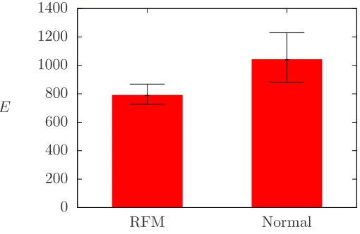
An initial analysis of 53 placental traces suggests that pregnancies with reduced fetal movement have lower efficiencies than those from normal preg-nancies (see figure 11). However, a protocol for producing traces needs to be developed and a more rigorous investigation carried out before we can place confidence in such results.
7.5 Discussion
7 INDEX OF EFFICIENCY FOR THE VASCULAR NETWORK 27
0 200 400 600 800 1000 1200 1400
RFM Normal
[image:27.595.180.435.137.303.2]E
Figure 11: Initial results for the efficiency index E for a set of placentas from 52 pregnancies, with 30 classified as having RFM and the remaining 23 normal.
cord covers part of the surface and therefore what looks like an area with no vascularisation (on the right of the umbilical insertion) is, in fact, an area lacking information.
The algorithm, although it gives an approximation of distance, does not take into account increasing distance along the diagonals. However, this inaccuracy is small in comparison to the noise in the input traces. In addi-tion, although the pixel size has been taken into account in calculating the index, the resolution varies between pictures. A protocol for photograph-ing and tracphotograph-ing the network would go a long way to resolve these problems and it would be possible to revert to calculating the distance to the nearest tip. Even with the crude approximations described, we see a difference in the mean efficiencies of placentas associated with normal births and those associated with reduced fetal movement.
7 INDEX OF EFFICIENCY FOR THE VASCULAR NETWORK 28
(a)
d= 4.566 cm
E= 1039.287
(b)
d= 5.969 cm
E= 848.575
(c)
d= 3.953 cm
E= 1506.379
(d)
d= 5.754 cm
[image:28.595.134.476.132.577.2]E= 913.162
29
Part III
Mathematical Modelling
8
Mechanical model to quantify the blood flow
8.1 Introduction
Assuming that the baby’s blood is sufficiently well bathed in the mother’s blood during transit, it will become fully oxygenated during its transit through the placenta. Thus the question of how efficient is a given pla-centa is how much flow can travel through the plapla-centa for a given pressure drop between the arteries and the vein in the umbilical cord. The cord will only be able to tolerate a given pressure drop, and this places a maximum on the blood that can flow through the placenta. In this section we develop a network model of the vessels that are visible on the ultrasound image and use a porous medium model of the unseen vessels. For the large vessels we assume they are rigid and contain Poiseuille flow, and in the small vessels we neglect effects of compliance. With these assumptions the overall model is linear, meaning that the total flow through the placenta is proportional to the overall pressure drop between the arteries and the vein in the umbilical cord. Our aim in this section is to develop rules for finding the constant of proportionality.
8.2 Porous medium model of blood flow in the placenta
8.2.1 Model development and simplification
We assume that a two-dimensional image of the shape of a placenta and tracings of the major vessels are provided, and attempt to use this to pre-dict the blood flow through the given placenta. We treat flow in the small arterial and venous vessels within the placenta as flow in two porous me-dia, following work by Chernyavsky et al. (2010) in which a more detailed porous medium model of a single lobule was considered, and by Bonfiglio
8 MECHANICAL MODEL OF THE BLOOD FLOW 30
lobule was modelled. We assume that the terminal end points of the visible vessels act as point sources for the arterial flow and point sinks for the venous flow (thus the invisible vessels are treated as part of the porous medium). In this section we prescribe the fluxes, but in Section 8.3 we develop a model that can be solved to find them. We denote the flux out of theith arterial vessel end byQai and that into the ith venous vessel end byQvi.
The flows in the arterial and venous networks are governed by Darcy’s equation:
ua=−
ka
µ∇pa, uv =− kv
µ∇pv, (8.1)
where ua is the spatially averaged arterial velocity, ka is the arterial
per-meability andpa is the pressure in the arterial vessels, and similarly for the
venous vessels (but with subscriptv) andµ is the blood viscosity. We also apply mass conservation for the arterial and venous vessels respectively:
∇ ·ua=−λ(pa−pv), ∇ ·uv =λ(pa−pv), (8.2)
where λ is the volume flux of blood transferring from the arterial to the venous vessels per unit volume of tissue per unit pressure drop between the arterial and venous vessels. Note that positive divergence indicates creation of mass and negative divergence indicates loss of mass. The boundary con-ditions are no flux of blood through the outer boundary of the placenta, that is ˆn·ua= ˆn·uv = 0 at the boundary.
Introducing p1 =pa−pv and p2=kapa+kvpv, we obtain
∇2p1−K2p1= 0, ∇2p2= 0, (8.3)
whereK2 =µλ(k−1
a +kv−1). Noting thatp1 and p2 can only be singular at the point sources and sinks with at most a logarithmic singularity at these points,p1 and p2 must have the form
p1= ˜p1+
X
vesselsi
AiK0(Kri), p2 = ˜p2+
X
vesselsi
Bilnri, (8.4)
where ri is the distance to the ith source/sink, Ai and Bi are constants,
K0 is a modified Bessel function of zeroth order and ˜p1 and ˜p2 are analytic functions. We enforce
I
Ci
ˆ
ni·uadl=
Qai
h ,
I
Ci
ˆ
ni·uvdl=−
Qvi
8 MECHANICAL MODEL OF THE BLOOD FLOW 31
where h is the depth of the placenta (assumed constant) andCi is a small
circle around the end of the vessel, and obtain
I
Ci
ˆ
ni· ∇p1dl=−
µ h
Qai
ka
+Qvi kv , I Ci ˆ
ni· ∇p2dl=
µ
h(Qvi−Qai). (8.6) In turn this means that, for alli,
Ai =
µ 2πh
Qai
ka
+Qvi kv
, Bi =
µ
2πh(Qvi−Qai). (8.7)
Since during development the lobule grows as a whole, it is reasonable to assume that it is not possible to transfer from one lobule to another during one transit of the placenta. In turn this means that Qai =Qvi =Qi, and
hence
Ai=
K2Q
i
2πhλ, Bi= 0. (8.8)
The boundary conditions become ˆn· ∇p1 = ˆn· ∇p2 = 0 at the boundary,
which implies that ˜p2 is constant, and we may take it to be zero by fixing the gauge pressure.
8.2.2 Statement of the simplified problem
The problem to be solved for ˜p1 reads
∇2p˜1−K2p˜1 = 0 (8.9)
in the placenta, subject to
ˆ
n· ∇p˜1 =− K
2
2πhλ
X
vessels i
Qinˆ· ∇K0(Kri) (8.10)
= K
3
2πhλ
X
vessels i
Qinˆ·ˆtiK1(Kri) (8.11)
on the boundary of the placenta, wheretiis the vector from the source/sink
to the point of interest, ri =|ti| and ˆti =ti/ri. Note that K′0 =−K1 and I′
0= I1 (Abramowitz & Stegun, 1964, equation 9.6.27). Once ˜p1 is found we find
pa=
kv
ka+kv
p1, pv =−
ka
ka+kv
p1, ua=−
λ
K2∇p1, uv = λ K2∇p1,
8 MECHANICAL MODEL OF THE BLOOD FLOW 32
where
p1= ˜p1+ K2 2πhλ
X
vessels i
QiK0(Kri). (8.13)
Note that, since there are singularities in the pressure at the ends of the ves-sels, we can only estimate the pressure in the vessels by finding the pressure on a circle about the singularity whose radius equals the vessel radius.
8.2.3 Special case with exact solution
The simplest case of a single vessel (the umbilical cord) in the centre of a circular placenta of radius R, that is the case when no vessels are visible, can be solved exactly to give
p1= K2Q1
2πhλ
K0(Kr) +
K1(KR) I1(KR)
I0(Kr)
, (8.14)
ua=−uv =
KQ1 2πh
K1(Kr)−
K1(KR) I1(KR)
I1(Kr)
. (8.15)
In this case we may estimate the pressure drop at the umbilical cord as
pa|r=ρa−pa|r=ρv =
kv p1|r=ρa+kap1|r=ρv
ka+kv
(8.16)
= µQ1 2πh
K0(Kρa)
ka
+K0(Kρv) kv
+K1(KR) I1(KR)
I0(Kρa)
ka
+ I0(Kρv) kv
,(8.17)
where ρa and ρv are respectively the radius of the arteries and vein in the
umbilical cord (note we need to assume the two arteries are the same size for the model to work).
In order to understand this solution better, consider the case in which KL ≪ 1 for typical length scales L within the placenta (note that this approximation is not yet justified). Using
I0(z) = 1 +O(z2), (8.18)
K0(z) =−ln
z
2
−γ+O(z2), (8.19)
I1(z) = z 2 +O(z
3), (8.20)
K1(z) = 1
8 MECHANICAL MODEL OF THE BLOOD FLOW 33
(Abramowitz & Stegun, 1964, equations 9.6.10–13), whereγ is Euler’s con-stant gives
p1 ≈ K2Q
1 2πhλ
2
K2R2 −ln
Kr 2 −γ , (8.22)
ua=−uv ≈
Q1 2πrh
1− r 2
R2
. (8.23)
Note that the non-zero divergence ofuaand uv, which represents transport
from the arterial to the venous system, appears clearly in the second term in the bracket.
8.2.4 Method to find the solution in the case of a general placenta and vessels
In this section we set up a method to find numerical solutions of (8.9). Working in polar coordinates (r, θ) centred on the umbilical cord (actually it could be any point if preferred), we can write the general solution of (8.9) as
˜ p1 =
∞
X
m=0
Im(Kr)
Amcosmθ+Bmsinmθ
(8.24)
whereAm, Bm ∈R,B0 = 0. Numerically, it is not possible to work with the infinite series (8.24), and so we truncate atM terms:
˜ p1=
M X
m=0
Im(Kr)
Amcosmθ+Bmsinmθ
, (8.25)
and thus we need to find 2M+1 unknown constantsAmandBm that satisfy
the boundary condition (8.11) as closely as possible.
We denote the locations of the ends of the terminal vessels by (Xi, Yi)
in Cartesian coordinates, and approximate the boundary of the placenta by a polygon withNp vertices at the points (xl, yl), l= 1,2, . . . , Np, which are
arranged in anticlockwise order around the boundary. At the midpoint of thelth edge, the point
t0l=
xl+xl+1
2 ,
yl+yl+1 2
, (8.26)
where we identify (xNp+1, yNp+1) with (x1, y1), the normal vector is given,
respectively in Cartesian and polar coordinates, by
ˆ
nl=
1 Rl
8 MECHANICAL MODEL OF THE BLOOD FLOW 34
= 1
r0lRl
xlyl+1−xl+1ylˆr+
1 2 x
2
l −x2l+1+y2l −yl2+1
ˆ
θ
,(8.27)
whereRl= p
(xl+1−xl)2+ (yl+1−yl)2 is the distance between
neighbour-ing vertices and r0l = |t0l|. At this point the boundary condition (8.11)
states
1 r0lRl
M X
m=0
Alm+
1 2r0lBlm
= K
3
2πhλRl X
vesselsi
Qi
rilXil
K1(Kril), (8.28)
where
Alm= (xlyl+1−xl+1yl)KI′m(Kr0l)
Amcosmθ0l+Bmsinmθ0l
(8.29)
Blm= x2l −x2l+1+y2l −yl2+1
mIm(Kr0l)
×Bmcosmθ0l−Amsinmθ0l
(8.30)
Xil=
xl+xl+1
2 −Xi
(yl+1−yl)−
yl+yl+1 2 −Yi
(xl+1−xl) (8.31)
and
til=
xl+xl+1 2 −Xi,
yl+yl+1 2 −Yi
(8.32)
is the vector from the ith vessel end to the lth midpoint, and ril = |til|,
θ0l= arg(t0l). Choosing 2M+1 different values ofl(for example by choosing
Np = 2M+ 1 and using the midpoints of all the edges), we obtain 2M + 1
linear equations (8.28) that can be used to determine the 2M+ 1 constants Am and Bm. Substituting these into (8.25) gives an approximation for ˜p1, and hence we may use (8.13) and (8.12) to find the approximate pressure and flux per unit area in the arterial and venous networks.
8.3 Network model of the large vessels
We assume that we have an image of the major arteries (or equivalently of the veins, which we assume are following the same paths as the arter-ies). Suppose there areNv arteries (or equivalently veins) on the image and
number these from 1 toNv, such that vessels 1 to Nu are attached directly
to the umbilical cord, vessels Nu + 1 to Niv are the other vessels that are
not terminal and vesselsNiv+ 1 to Nv are terminal. We assume that each
bifurcation has one parent and two daughter vessels, that arteryihas length Li and diametersDaiand therefore vein ialso has lengthLi and we denote
8 MECHANICAL MODEL OF THE BLOOD FLOW 35
and d2(i), where d1,2 :{1,2, . . . , Niv} 7→ {Nu + 1, Nu+ 2, . . . , Nv} and the
parent vessel of vessel i by p(i), where p :{1,2, . . . , Nv} 7→ {0,1, . . . , Niv}
(we setp(i) = 0 for vessels 1, . . . Nuthat are attached to the umbilical cord).
Thus i=p(d1(i)) =p(d2(i)) for i= 1, . . . , Niv and i is equal tod1(p(i)) or d2(p(i)) fori=Nu+ 1, . . . , Nv.
We denote by Qi the flux through the ith artery and by Q0 the flux through the two arteries in the umbilical cord. Since the flux exiting the terminal artery equals that of the corresponding vein, the fluxes in vein i must equal Qi over the whole network, and the flux in the vein in the
umbilical cord equals Q0. We let Pai be the pressure at the distal (to the
fetus) end of arteryi(i= 1, . . . , Nv) andPa0 be the pressure in the arteries in the umbilical cord (we assume the two arteries have equal pressures). and Pvi be the pressure in the distal end of veiniandPv0 be the pressure in the vein of the umbilical cord. We letPai−Pvi=Pi.
Mass conservation at the umbilical cord implies that
Q0 =
Nu
X
i=1
Qi, (8.33)
and mass conservation at the distal end of theith vessel implies
Qi =Qd1(i)+Qd2(i), fori= 1, . . . , Niv. (8.34)
The porous medium model provides the relationships
Pi=Pai−Pvi=
Nv
X
j=Niv+1
ΛijQj, fori=Niv+ 1, . . . , Nv, (8.35)
where we solve for ˜p1 for the case Qk = δjk (that is all the Qk’s are zero
exceptQj, which equals 1), and set Λij to be the value ofp1 at theith vessel end, which, from (8.13), is
Λij =
˜
p1|vesseli+
K2 2πhλ
kvK0 12KDai
+kaK0 12KDvi
ka+kv
fori=j,
˜
p1|vesseli+ K 2
2πhλ K0(Krij) fori6=j,
(8.36) where rij is the distance between the ith and jth vessel ends. Finally,
momentum conservation in theith artery and theith vein gives respectively
8 MECHANICAL MODEL OF THE BLOOD FLOW 36
where Γai = 128µLi/πDai4 and Γvi = 128µLi/πD4vi are the Poiseuille
resis-tances. Combining these
Pp(i)−Pi= (Γai+ Γvi)Qi, fori= 1, . . . , Nv. (8.38)
Equations (8.33)–(8.35) and (8.38) represent 2Nv+ 1 linear equations for
the 2Nv+ 2 variables Pi and Qi, i= 0,1, . . . , Nv. Setting P0 = 1 provides sufficient information to calculateQ0. The valueQ0thus calculated provides a measure of the conductivity of the placenta.
8.4 Parameter estimation
In order to use the model, certain parameters must be found, which are listed in this section. Using the image we can find the numbers of vesselsNu,Niv
and Nv, the relationships defining the bifurcations, p(i), d1(i) and d2(i), and the lengths Li. We also require measurements of the vessel diameters
Dai andDvi, and these necessitate further image processing. In addition we
need estimates of the blood viscosity, µ, the Darcy permeabilities, ka and
kv, the flow rate per unit pressure drop,λ, and the placenta height, h.
Figure 13 shows the output of the numerical code on an idealised pla-centa, demonstrating the feasibility of the method. This is done with made-up parameter values. In future work we will estimate these parameters from the literature, and use them to predict the placental blood flow for images of real placentas.
8.5 Discussion
The porous medium model neglects several aspects of the placenta. Crucially the model assumes that arteries and veins lie along the same tracks, which is unlikely to be true in practice. A further complication is that each lobule is not necessarily supplied by either a single major artery and/or drained by a single vein. The assumption that arteries and veins are in the same place is likely to have a significant effect on the quantitative predictions of the model; nevertheless, there is likely to be a good correlation between the ranks of the efficiency predicted by the model and the true efficiency of the placenta. If it were possible to identify separately the arteries and veins on the image, this would significantly improve the predictive capability of the model.
8 MECHANICAL MODEL OF THE BLOOD FLOW 37
Pressure difference between arteries and veins
−0.1 −0.05 0 0.05 0.1
−0.08 −0.06 −0.04 −0.02 0 0.02 0.04 0.06 0.08
[image:37.595.146.465.138.389.2]3 3.5 4 4.5 5 5.5 6 6.5 x 10⁻⁶
Figure 13: Distribution of the pressure difference p1 in an idealised
pla-centa, based on a simplified version of the placenta in the fileNORMAL2. The
boundary of the idealised placenta (in this case a circle) is shown by the black line (using 51 vertices) and the approximate locations of the ends of the vessels are shown by the black asterisks. The parameter values used are µ= 0.004 Pa s,λ= 0.1 (Pa s)−1, ka = kv = 5×10⁻⁵m2, h = 3 cm. Every
vessel is treated as having length2 cmand diameter 1 mm
drop, and so it is important to use an accurate estimate of the diameter of a vessel. The model also does not differentiate between the two arteries supplying the placenta, but this is unlikely to have a significant effect since the pressures of the blood in these vessels are similar. Currently we must estimate parameters of the network of vessels from the image of the pla-centa; however, in future work we plan to automate retrieval of the required parameters.
8 MECHANICAL MODEL OF THE BLOOD FLOW 38
for the fetuses because these can have a large pressure drop along their length, leading to loss of blood from one fetus to the other. Franke et al.
9 DEVELOPMENT OF THE VILLOUS TREE 39
9
Modelling the development of the villous tree
In this section, we propose a model for the normal growth and development of the human placenta. The objectives are to understand the abnormal pat-terns seen in complicated pregnancies. Background about the development of the villous tree can be found in§2.
9.1 Modelling the villi growth rate as linearly dependent on nutrients
A simple model is presented here on the growth of the placenta. The initial time is chosen to be when the placenta has differentiated into around 5 villi and has just started sending blockers into the spiral arteries immediately located opposite the villi. This is around time t = 4 weeks. Clinical ob-servations suggest that the diameter of the surface covered by these villi is approximately 2 centimetres in diameter at that time. Assume that five villi of that size have formed already in a star shape as shown in figure 14. The radius and coordinates of the boundary is given by
rvilli= (0.3 + 0.15 cos 5θ) cm, (9.1)
x y
= (0.3 + 0.15 cos 5θ)
cosθ sinθ
cm. (9.2)
For the next 6 weeks the uterus grows in order to accommodate for the developing fetus. The model assumes that this growth is independent of the development of the placenta and the parameters are chosen to represent a uterus of size 5×5×5 cm3 in week 4 and 10×10×7 cm3 in week 10. These values are based on clinical observations. The radius of the uterus is thus defined by
ruterus(t) =
2.5 + (5−2.5)t/weeks−4 6
cm, (9.3)
wheretis measured in weeks.
9 DEVELOPMENT OF THE VILLOUS TREE 40
Figure 14: Development of villi in the placenta and the surface of the uterus, which is covered by spiral arteries delivering nutrients uniformly to the placenta, between the 4th and 10th weeks of pregnancy.
and structure of the uterus is very complicated. For simplicity, it will be assumed that the embryo is in a position in the uterus where, by symmetry, it receives the same nutrients in all directions. This can be modelled by saying the surface of the uterus, which is covered by spiral arteries delivering nutrients to the placenta, is circular with the villi positioned in its centre.
9 DEVELOPMENT OF THE VILLOUS TREE 41
that deliver more nutrients on one side rather than another to the placenta. For simplicity, consider such a case where the uterus is still circular but the position of the placenta is off its centre. The initial condition of the villi is then given by
x y
=
x0 y0
+ (0.3 + 0.15 cos 5θ)
cosθ sinθ
cm. (9.4)
Such a solution is shown in figure 15 for the off-centre values x0 = 0.7, y0 = −1.9. It shows that the villi tend towards a circular shape but do not manage to reach that by the 10th week and remains as an elliptical shape. The size of the placenta at the final time is slightly smaller than that in the solution in figure 14, but is still of similar magnitude. There are clinical observations of placentas that are elliptical in shape and smaller in size that perform worse than those that are regular. So the hypothesis that the function of the placenta may decline due to an irregular development of the villi is worth considering further. However, many assumptions have been made in this model that need revising. These include the circular shape of the uterus, the immediate deactivation of the spiral arteries, the linear growth relationship of the placenta to the nutrients in the system and the uniform distribution of nutrients in the decidua around the spiral arteries. An attempt to develop a more sophisticated model was made during the study group but was not finished due to time restrictions. A brief overview is presented next.
9.2 Modelling the development of the villi using chemotaxis and diffusion
9.2.1 General equations
The shape of the uterus is modelled as growing linearly in time again with the same rate and form as in (9.3). However, the difference in this model is that the growth of the placenta is not assumed to be linearly proportional to uniformly-distributed nutrients in the decidua, but is driven by chemotaxis toward areas of high concentration of these. The decidua can be modelled as consisting of nutritional sources and sinks, representing the spiral arteries and maternal veins. Let these positions be labelled asxnfor the sources and yn for the sinks. Let T(x, y, t) be the cells on the embryonic side that are forming villi, Tc(x, y, t) the position of the boundary of the T(x, y, t)-cells
9 DEVELOPMENT OF THE VILLOUS TREE 42
Figure 15: Development of villi in the placenta and the surface of the uterus, which is covered by spiral arteries delivering nutrients to the placenta in a non-uniform way, between the 4th and 10th weeks of pregnancy.
set of differential equations that can describe the system is
∂a
∂t =D1∇
2a+X
n
knfn(xn, Tc)δ(x−xn)
−X
m
lmgm(xm, Tc)δ(x−ym)−c1(a)−c2(T), (9.5)
∂T
∂t =D2∇ 2T
−∇ ·(χT∇a)−c3(T) +c4(T). (9.6)
The constantsD1,2 are the diffusion rates for the distributionsa(x, y, t) and T(x, y, t) respectively. The constants kn and lm represent the strength in
9 DEVELOPMENT OF THE VILLOUS TREE 43
a(x) concentration
[image:43.595.189.434.130.255.2]T(x, t) cells
Figure 16: A diagram of the spiral arteries being blocked by hormones sent from the villi. This process is modelled by switching off all spiral arteries covered by the villous cells. The black outline in the second row represents the boundary of these cellsTc. The dots in the first row represent positions
of spiral arteries.
might give better results. The strength of ‘attraction’ of the villous cells toward nutrients is measured by the chemotactic term χ. This can be a function of space, but for simplicity will be assumed to be constant. The functions c1(a) and c2(T) represent oxygen uptake by the decidual tissue and villous cells respectively. The termsc3(T) and c4(T) are the death and birth rates of theT(x, y, t)-cells. These can probably be neglected without much change in the solution since the growth is modelled by the diffusion rather than by the number of villi. Finally, the function fn(xn, Tc) is the
non-linear term in the equations that represents the blocking and unblocking of spiral arteries and maternal veins. It has the property that it is 0 when the hormones have been released to block the arteries directly underneath the villi and 1 when they have not. Mathematically, it can be represented as
fn(xn, Tc) =
1 : xn∈/Tc,
0 : xn∈Tc. (9.7)
The termgm is similar to fn but relates to the maternal veins rather than
spiral arteries. Both their functions are described by the diagram in fig-ure 16.
9.2.2 First simplification
9 DEVELOPMENT OF THE VILLOUS TREE 44
solution quantitatively rather than qualitatively and also are not the key ones in the problem to be modelled. An uptake termc1(a) is needed in the first equation to balance the diffusion term. Thus they can be neglected. The simplest possible form that can be taken is a linear relationship in a(x, y, t). However, other forms should also be considered in the future. In addition, the oxygen concentration can be assumed to be steady in time as it is assumed that the spatial distribution will not vary greatly in time. This assumption is realistic for short timescales when the uterus is of constant size and the locations of the sources and sinks do not change. Then the system of equations can be simplified to
0 =D1∇2a+
X
n
knfn(xn, Tc)δ(x−xn)
−X
m
lmgm(xm, Tc)δ(x−ym)−c1a , (9.8)
∂T
∂t =D2∇
2T −∇ ·(χT∇a) , (9.9)
where c1 is the rate of uptake. The first equation in this system is non-linear but can be solved as a non-linear problem at each time-step. This means that it is possible to obtain a solution for the oxygen distribution by taking the effect of diffusion and a single source term and then linearly adding all sources together at every time step. Without loss of generality, consider all sinks to be 0 and that the sources can also represent sinks if the strength constantskn can be taken to be negative.
9.2.3 Nutrient concentration with a single central source
Consider a source singularity in two-dimensional space that produces a con-centration of nutrients that satisfy
0 =D1∇2a−c1a , (9.10)
subject to ∂a/∂r = 0 at r = 1 and a singularity condition at r = 0 such that the flux through that point is some constant Q. The general solution to (9.10) is
a(x, y) =A I0
r
c1 D1
r
+B K0
r
c1 D1
r
, (9.11)
9 DEVELOPMENT OF THE VILLOUS TREE 45
The boundary condition then yields
A=B K1 q c1 D1 I1 q c1 D1 . (9.12)
Finally, the flux condition gives
I
(−∇a)·ndl=Q ⇒ Q=−lim
ǫ→0
Z 2π
0 ∂a ∂r
r=ǫ
ǫdθ= 2πB ,
(9.13) which determines the constantBand yields a full solution. Solving the same problem for a general source that is not atr= 0 is a lot harder and was not done during the study group. There was an idea to change the coordinate system from (r, θ) to one with an origin at the source and the hope that the boundary condition will work out, but that analysis was not finished due to time constraints.
9.2.4 Nutrient concentration with a single off-centre source
A third attempt was made to solve the following problem
0 = D1∇2a−c1a+Q δ(r−R)δ(θ−Θ) (9.14)
|∇a| →0 as r→0, (9.15)
∂a
∂r = 0 at r= 1. (9.16)
Using separation of variables the general solution to the homogeneous ver-sion of (9.14) (i.e. with Q=0) is
a(r, θ) =X
n
An In
r c
1 D1
r
+Bn Kn
rc
1 D1
r
×Cnsin(nθ) +Dncos(nθ)
. (9.17)
We then consider separate solutions based on (9.17) in 0 < r < R and R < r <1, and apply the matching conditions
[a]RR+−= 0, (9.18)
∂a ∂r
R+
R−
=− Q D1
9 DEVELOPMENT OF THE VILLOUS TREE 46
Applying the boundary conditions (9.15) and (9.16) together with the first matching condition (9.18) and ensuring symmetry aboutθ= Θ, we obtain
a(r, θ) =
1
2a0f0(r)g0(R) + ∞
X
n=1
anfn(r)gn(R) cos
n(θ−Θ) : r < R
1
2a0f0(R)g0(r) + ∞
X
n=1
anfn(R)gn(r) cos
n(θ−Θ) : r > R
(9.20) where
fn(r) = In r c1 D1 r , (9.21)
gn(r) =
In q
c1
D1r
I′ n q c1 D1 − Kn q c1
D1r
K′ n q c1 D1 . (9.22)
Thean are determined by applying the final matching condition (9.19). In
what reduces to finding the Fourier series forδ(θ−Θ), we obtain
an= −
Q πD1
fn(R)gn′(R)−fn′(R)gn(R)
−1
. (9.23)
9.2.5 Multiple off-centre sources
In principal, a solution could now be built for multiple sources, by super-posing a number of copies of this solution with different values of Q, Θ, R. However, owing to a lack of time, there was no further investigation of this at the study group.