On the detection of nearly optimal solutions in the context of single-objective space mission design problems

context of single-objective space mission design problems. Proceedings

of the Institution of Mechanical Engineers, Part G: Journal of Aerospace

Engineering, 225 (11). pp. 1229-1242. ISSN 0954-4100 ,

http://dx.doi.org/10.1177/0954410011413693

This version is available at https://strathprints.strath.ac.uk/38309/

Strathprints is designed to allow users to access the research output of the University of Strathclyde. Unless otherwise explicitly stated on the manuscript, Copyright © and Moral Rights for the papers on this site are retained by the individual authors and/or other copyright owners. Please check the manuscript for details of any other licences that may have been applied. You may not engage in further distribution of the material for any profitmaking activities or any commercial gain. You may freely distribute both the url (https://strathprints.strath.ac.uk/) and the content of this paper for research or private study, educational, or not-for-profit purposes without prior permission or charge.

Any correspondence concerning this service should be sent to the Strathprints administrator:

[email protected]

The Strathprints institutional repository (https://strathprints.strath.ac.uk) is a digital archive of University of Strathclyde research outputs. It has been developed to disseminate open access research outputs, expose data about those outputs, and enable the

http://pig.sagepub.com/

Engineering

Engineers, Part G: Journal of Aerospace

http://pig.sagepub.com/content/225/11/1229

The online version of this article can be found at:

DOI: 10.1177/0954410011413693

originally published online 23 September 2011

2011 225: 1229

Proceedings of the Institution of Mechanical Engineers, Part G: Journal of Aerospace Engineering

O Schütze, A Lara, C A Coello Coello and M Vasile

problems

On the detection of nearly optimal solutions in the context of single-objective space mission design

Published by:

http://www.sagepublications.com

On behalf of:

Institution of Mechanical Engineers

can be found at:

Proceedings of the Institution of Mechanical Engineers, Part G: Journal of Aerospace Engineering

Additional services and information for

http://pig.sagepub.com/cgi/alerts Email Alerts:

http://pig.sagepub.com/subscriptions Subscriptions:

http://www.sagepub.com/journalsReprints.nav Reprints:

http://www.sagepub.com/journalsPermissions.nav Permissions:

http://pig.sagepub.com/content/225/11/1229.refs.html Citations:

What is This?

- Sep 23, 2011

OnlineFirst Version of Record

- Nov 16, 2011

Version of Record

On the detection of nearly optimal solutions in

the context of single-objective space mission

design problems

O Schu¨tze1, A Lara1, C A Coello Coello1,andM Vasile2*

1_{Computer Science Department, CINVESTAV-IPN, Mexico City, Mexico} 2

Department of Mechanical Engineering, University of Strathclyde, Glasgow, UK

The manuscript was received on 2 November 2010 and was accepted after revision for publication on 24 May 2011.

DOI: 10.1177/0954410011413693

Abstract: When making decisions, having multiple options available for a possible realization of the same project can be advantageous. One way to increase the number of interesting choices is to consider, in addition to the optimal solution x*, also nearly optimal or approximate solutions; these alternative solutions differ from x* and can be in different regions – in the design space – but fulfil certain proximity to its function valuef(x*). The scope of this article is the efficient computation and discretization of the setEof e–approximate solutions for scalar optimization problems. To accomplish this task, two strategies to archive and update the data of the search procedure will be suggested and investigated. To make emphasis on data storage efficiency, a way to manage significant and insignificant parameters is also presented. Further on, differential evolution will be used together with the new archivers for the computation ofE. Finally, the behaviour of the archiver, as well as the efficiency of the resulting search procedure, will be demonstrated on some academic functions as well as on three models related to space mission design.

Keywords: single objective optimization, approximate solutions, differential evolution, space mission design

1 INTRODUCTION

One common way to solve a real world engineering problem is by transforming it into an optimization problem (without loss of generality, we assume in the sequel minimization problems) and to seek for the (or at least one) optimal solution. From a practical point of view, however, it can, in some cases, make sense to include (in addition to the optimal solutions) also nearly optimal solutions since this will give the decision maker (DM) a larger variety of possibilities:

two solutions which are ‘near’ in objective space (i.e. have similar objective values) may differ significantly in parameter space. The storage of both solutions may give the DM a second option for the realization of his/her project.

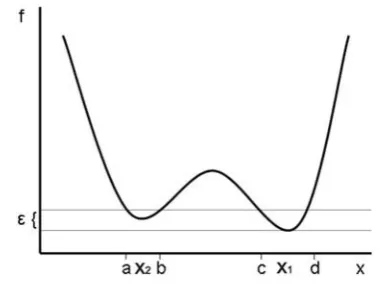
As one example, consider the objective shown in Fig. 1. In case, the DM is willing to accept a deterio-ration ofe2IR_þ, the objective functionfcontains next to the global minimizerx1also the local minimizerx2

which is such an ‘e-approximate solution’ (i.e. the function values of f(x1) and f(x2) differ by less

than e). All other points in [a,b][[c,d] are also approximate solutions, however, they are all ‘domi-nated’ (i.e. they offer worse values off) within their connected components by the solutions x1 and x2.

Hence, these solutions are possibly too near to

these two points in order to give the DM a significant new alternative. This depends on the minimal dis-tance that these two solutions must keep from each other in order to be considered as ‘distinct’ from a practical point of view.

Hence, an ‘optimal’ outcome of the optimization process (depending on the problem) could be to pre-sent the possible choices x1 and x2 – and no other

solution to avoid confusing the DM and for the sake of an efficient computation (since no superfluous options have to be stored and updated).

As another example, consider the problem of designing an ‘optimal’ trajectory from Earth to the comet 67P/Churyumov-Gerasimenko (see references [1,2], and also section 5.4). One crucial parameter is the launch dateT0which is in the time window [1460,

1825] MJD2000 (Modified Julian Date 2000). The best known solution is a trajectoryP1 withT0(P1)¼1546

[MJD2000] (value rounded) and objective value

f(P1)&1.34 [km/s] (measured as the total variation

in velocity that the engines have to deliver to reach the destination). If the DM is willing to accept a dete-rioration of e¼0.5 [km/s], then he/she is given (among others) another two possible local optimal trajectories P2 (with T0(P2)¼1619 [MJD2000] and

f(P2)¼1.76 [km/s]) and P3 (with T0(x3)¼1748

[MJD2000] and f(x3)¼1.76 [km/s]). Hence, in that

case, the DM is offered two more choices for the launch of the spacecraft (2.5 respectively 6.5 months afterT0(P1)).

In this article, the problem of computing approxi-mate solutions of scalar optimization problems is addressed. Since the set E of these e-approximate solutions typically forms an-dimensional set, where

nis the dimension of the parameter space, a suitable discretization is mandatory in order to be applicable to real world problems. In this study, the focus will be on the approximation of the local minima within E.

However, also further points will be considered. If, for instance, the objective is ‘flat’ around a local mini-mum inE(as, for instance, happens for the ‘funnels’ in models related to space mission design), then also points which are not locally optimal but differ suffi-ciently in parameter space from the local solutions could be interesting for the DM. To achieve this goal, two archiving strategies (i.e. strategies to main-tain a subset of the obmain-tained data) will be proposed and investigated. In order to obtain an efficient algo-rithm for the approximation ofE, the archivers will be combined with differential evolution (DE), a heuristic that has already shown its efficiency on space mission design problems [3,4].

This study can be considered as an ‘extension’ of previous studies on the computation of approximate solutions for multi-objective optimization problems (MOPs) [5–7]. The crucial difference when consider-ing scalar optimization problems (i.e. one objective) is that in that case, a discretization in parameter space can be performed. As will be seen later on, a discretization of the set of interest is mandatory. In case multiple objectives are under consideration, a discretization in parameter space leads either to a tremendous number of archive entries when choos-ing small or even moderate values for the discretiza-tion parameter, or leads to grave loss of informadiscretiza-tion in case this parameter is large. The latter is due to the fact that the solution set (the so-calledPareto set) typ-ically forms a (k1)-dimensional object, wherekis the number of objectives in the MOP, and hence, a discretization around a promising point (optimal or nearly optimal) leads to a non-observance of an entire (and large) optimal region. This will change, however, if we consider only one objective since in that case the (local or global) optima are typically isolated (as in Fig. 1). Thus, in such case, a discretization can in prin-ciple be performed in parameter space without essential loss of information. A preliminary study of this can be found in reference [8].

Next, there is a certain relation to multi-modal optimization [9–17], where the task is to detect all local minima within a given region. However, note that there are some differences to the approach in this study: first, this study is not interested in local minima nor any other point outsideE. Second, and that is more important, the present study is not ‘restricted’ to local minima (though better solutions in a given neighbourhood will be preferred in order to discretize the set of interestE). For this, consider for instance Rosenbrock’s banana function (which indeed shares some characteristics with the objec-tives related to space mission design considered in this study). The function contains one global min-imummwhich is located inside a long, narrow, and

Fig. 1 Example of an objective function with two local minimax1andx2which are similar in objective

flat valley. Hence, it could make sense to compute next tom(as for multi-modal optimization) also fur-ther approximate solutions along the valley, since they could be distinct solutions for the DM.

Finally, approximate solutions in space mission design problems have already been considered in reference [18], where a hybrid multiagent approach has been chosen for their detection.

The remainder of this article is organized as follows: section 2 gives the required background for the understanding of the sequel. Section 3 presents and investigates the set of interest, and in section 4 methods are proposed for their efficient computation. Section 5 presents some numerical results, and finally, some conclusions are drawn in section 6.

2 BACKGROUND

In this article, we consider single-objective optimiza-tion problems (SOPs) of the following form:

min

x2Q fðxÞ ð1Þ

where it is assumed thatf:QIRn_!IR is continuous. For theoretical purposes, it has to be assumed thatf

is even continuously differentiable, though this smoothness assumption will never be used in the numerical treatment (since DE does not exploit gra-dient information). Further, it has to be assumed that the domainQis compact which is typically given ifQ

is defined by equality and inequality constraints. In the easiest case (which is already sufficient for the models considered in this study), Q can be defined by box-constraints, i.e. the domain forms ann-dimensional box

Q_¼x₂Rn : _ai4xi4bi,i¼1,. . .,n ð2Þ

whereai andbi are the lower and upper bounds of

each parameterxi.

The solution set of (1) is given by

MQ:¼ fx2Q : fðxÞ4fðyÞ 8y 2Qg ð3Þ

Note thatMQdoes not have to consist of one single

solution, however, except for plateau functions, the solution set will be a finite set of points (i.e. a 0-dimensional set). To illustrate this, the reader may think of the sine curve restricted to a closed interval. Algorithm 1 gives a framework of a generic stochas-tic search algorithm, which has first been studied in reference [19], and which will be considered in this study. Here, QIRndenotes the domain of the problem, Pj the candidate set (or population) of

the generation process at iteration stepj, andAjthe

corresponding archive.

Algorithm 1Generic Stochastic Search Algorithm

1:P0Qdrawn at random

2:A0¼ArchiveUpdate(P0,;)

3:forj_¼0, 1, 2,. . ._do 4: Pjþ1¼Generate(Pj)

5: Ajþ1¼ArchiveUpdate(Pjþ1,Aj)

6:endfor

Finally, some distances between points and sets as well as between different sets are defined which will be needed to evaluate the approximation quality of the outcome set.

Definition 2.1

Let u, v2IRnandA,BIRn. The semi-distance dist(,) and the Hausdorff distance dH(,) are defined as

follows:

(a) dist_ðu,A_Þ:_{¼infv2Akuvk;} (b) dist_ðB,A_Þ:_¼supu

2Bdistðu,AÞ;

(c) dH(A,B)9max {dist(A,B),dist(B,A)}.

3 THE SET OF INTEREST

In the following, the set of interest,MQ,e, is defined

and some of its topological properties are discussed.

Definition 3.1

Lete>0. x2Q is called ane-approximate solution of (1) iff(x)e4f(y) for all y2Q. The set ofe-efficient solutionsMQ,eof (1) is defined by

MQ, ¼ fx2Q : f ðxÞ 4fðyÞ 8y 2Qg ð4Þ A point x is ane-approximate solution of a setA if

f(x)e4f(a) for alla2A.

The following examples illustrate the set of interest.

Example 3.2

(a) Letf: IRn_!IR be given by fðxÞ ¼X

n

i¼1

xi2 ð5Þ

then the setsMQandMQ,efor ane>0 are given by

MQ¼ f0g, MQ,¼ x2Rn :

Xn

i¼1

x2

i4

( )

ð6_Þ

that is, MQ,eis the closed ball with centre 0 and

radiuspffiffiffi_.

(b) The set ofe-approximate solutions for the intro-ductory example (Fig. 1) is given by MQ,e¼

The following short discussion shows that MQ,eis

typically n-dimensional (whereas MQ is typically

0-dimensional): let x_2M Q\Q

, where Q denotes the interior of Q, and f is continuous. Then, there exists, by continuity of f, a neighbourhood N of x* insideQsuch that

f _ðx_Þ 4f_ðx_{Þ 8x2N ð7Þ}

and hence, the n-dimensional set N is contained in MQ,e. Thus, suitable discretization strategies are

required for the efficient use of approximate solutions.

Another important aspect is the connectedness of the set of interest. It can be shown (analogue to refer-ence [20]) that in case both the objective f as well as the domainQare convex, thenMQ,e is connected

(and can possibly be computed most efficiently by local search procedures if at least one solution is available), but this does not hold in general, as the above example shows. Hence, global strategies seem to be advantageous for the treatment of general objectives.

One potential problem at least for theoretical observations is that MQ,e may contain isolated

points. For this, consider the objective function shown in Fig. 2 which is a modification of the intro-ductory example: in this case, it isMQ,e¼{x*}[[c,d],

that is, contains the isolated point x*. The problem with such points is that it cannot be guaranteed to capture them by the use of stochastic search algo-rithms [20]. To allow convergence of the algorithm the following has to be assumed

BQ and _rf _ðx_{Þ 6¼}0₈x₂B _ð8_Þ where_rf(x) denotes the gradient offatx, andBthe boundary ofMQ,e, i.e. it holds

B:_{¼ fx2Qjf ðmÞ þ¼f ðxÞform2MQg ð9Þ}

Under this assumption, it can be shown (analogue to reference [20] that MQ,e contains no isolated

points, that is

MQ,¼MQ, ð10Þ

Finally, it is important to note that the approach can be used to detect multiple solutions inMQsince

every optimal solution is also an e-approximate solution. To be more precise, the set of optima MQ

is contained inMQ,efor everye>0. Furthermore, it is

MQ¼

\

40

MQ, ð11Þ

Classical elitist approaches have strong limitations in detecting multiple solutions since there is typically only one ‘best’ (scalar) value out of a finite set of can-didates. Regarding this, it is important to note that a discretization ofMQ,ecannot be performed by merely

considering the objective values (as e.g. done in reference [20] for the multi-objective case).

4 AN ALGORITHM FOR THE APPROXIMATION OFMQ,e

In this section, one possibility to compute approxi-mations of MQ,e – DE together with an external

archive – is presented. Following the notation of Algorithm 1, the archiver and the generator which constitute the stochastic search process will be con-sidered separately.

4.1 Two archiving strategies

In the following, two possible archiving strategies aiming for the representation ofMQ,e are discussed:

the first captures alle-approximate solutions out of the obtained data, and the second one uses a certain discretization strategy.

The first archiver considered here,

ArchiveUpdateMQ,e, is shown in Algorithm 2. The

information management is straightforward: the algorithm captures all the e-efficient solutions out of the obtained data (i.e. out of the sequence of can-didate setsPi). The following proposition states this

more precisely.

Proposition 4.1

Letl₂N,e2IR

þ,P1,. . .,PlIRnbe finite sets, andAi, i_¼1,. . ._{,l, be obtained by ArchiveUpdateMQ,}e as in

Algorithm 1. Then

Al ¼MCl, ¼ fx2Cl : f ðxÞ 4fðyÞ 8y2Clg

ð12_Þ whereCl ¼Sli_¼1Pi.

Proof

Follows by construction ofArchiveUpdateMQ,e. #

Next, the limit behaviour of the sequence of archives

Aigenerated by the archiver is investigated. For this,

the following assumption on the generation process has to be made [21,22]

8x₂Qand₈4₀:

Pð9l2N : _Pl\BðxÞ \Q6¼ ;Þ ¼1 ð13Þ where P(A˚) denotes the probability for event A. Assumption (13) says, roughly speaking, that every neighbourhood U_\Q of every point gets ‘visited’ byGenerate() after finitely many steps with probabil-ity one. The following consideration shows that we cannot assume less: if (13) does not hold, there exists with probability one a point x₂Q and a neighbourhood U˜_¼U_\Q of x such that no candidate solution p₂Pl lies in U˜ for all l2N.

Thus, no convergence can be guaranteed since a part ofMQ,ecan be contained inU˜ which is never

‘visited’.

Corollary 4.2

Let a SOPf: IRn!IR be given, where F is continuous, let QIRn be a compact set and e2IR

þ. Further,

let the assumptions (8) and (13) be fulfilled. Then, an application of Algorithm 1, where

ArchiveUpdateMQ,e is used to update the archive,

leads to a sequence of archivesAl,l2N, with

lim

l!1dHðMQ,,AlÞ ¼0, with probability one

ð14_Þ

Proof

The proof is analogue to the proof of Theorem 2 of reference [5] using the modified assumption (8). #

However, due to the dimension ofMQ,e, the strategy is

apart from a theoretical point of view only interesting, e.g. if the cost of a function evaluation is relatively high, i.e. if only a moderate amount of function calls can be spent within a given time budget. In that case, it makes sense to store all interesting information (and not to lose single promising candidates due to discretization) andArchiveUpdateMQ,ecan be chosen

without significant computational loss.

More interesting – and mandatory for the efficient application to real world problems – is certainly to filter the incoming data farther by considering a suit-able discretization strategy. In order to accomplish this task, ArchiveUpdateMQ,eDx (Algorithm 3) is

proposed here which is similar to the first archiver but performs a selection of the promising data. The underlying idea of ArchiveUpdateMQ,eDx is to keep

(locally) best found solutions within a certain range (usinge2IR

þin objective space and a vector2Rnþ

in parameter space) and to discard inferior points in the neighbourhood of these ones in order to obtain a suitable discretization (compare to the motivating example in section 1).

Algorithm 2A9ArchiveUpdateMQ,e(A0,P,e)

Require: archive A0, candidate set PQ, tolerance

e2IR_þ

Ensure: updated archiveA

1:A9A0

2:for allp2Pdo

3: if`a₂A:f(a)_þe4f(p)then 4: A9A[{p}

5: end if

6: for alla₂Ado

7: iff(p)_þe<f(a)then 8: A9A\{a}

9: end if

10: end for

11:end for

More precisely, given an archiveA0and a candidate

solution p, the new archiver A is constructed as follows: p is rejected (and hence, A is set to A0)

if either p is not an e-approximate solution of A₀ (i.e.f(xb)þe<f(p), where x_bis the best found solu-tion), or if there exists an element a₂A0\B1ðpÞ,

where the neighbourhoodB1

ðpÞis defined as

B1ðpÞ:¼ fx2R

n _:

jxipij5i, i¼1,. . .,ng

ð15Þ

which is at least as good as p (line 6 of Algorithm 4). If p is not discarded, this means that (i) this point is an e-approximate solution of A, and (ii) that it is the best point in its neighbourhood (the latter defined by_2Rn

þ). Hence, the new archiveA

consists ofp as well as all other points ofA0which

are e-approximate solutions of p, and which are not in the _{-neighbourhood of p (lines 10-14 of} Algorithm 3).

Note that ArchiveUpdateMQ,eDx in Algorithm 3

is formulated for the consideration of one candi-date point p. However, an extension to entire sets

PQ is straightforward. Further, for the sake of a better readability the best found solution xb

Algorithm 3{A,xb}9ArchiveUpdateMQ,eDx(A0,xb,0, p,e,)

Require: archive A0, best found solution xb,0,

candi-date solution p₂Q, tolerance e2IR

þ, discretization

parameter_2Rn

þ

Ensure: updated archiveA, best found solutionxb

1:iff(p)<_f(xb,0)then

2: xb9p

3:else

4: xb9xb,0

5:end if

6: if f(xb)þe<f(p) or (9a2A₀:p2B1ða_jÞ and

f(a)4f(p))then

7: A9Ao [discardp

8: return

9:end if

10:A9{p}

11:for alla₂A0do

12: iff(a)4f(xb)þeanda62B1ðpÞthen 13: A9A[{a}

14: end if

15:end for

Results of the sequence of archives when using

ArchiveUpdateMQ,eDx are not as straightforward as

for the first archiver ArchiveUpdateMQ,e. Given Al

and Cl as above, and denoting by xb,l to the best

found solution in stepl, then it holds

xb,l 2MCl and Al MCl, ð16Þ

However, further approximation qualities (such as the Hausdorff distance between Al and MCl,e) for

finite candidate solutions {p1,. . .,ps}, s2N, cannot

be given since the final archive Al depends on the

order the candidate solutions pi are considered.

For this, consider the following example: let f : [0, 10]_!IR,f(x)_¼x2, ande¼1. Then, it is M_Q,

e¼[0,

1]. Let a hypothetical candidate set be given by

P1¼ f0, 0:05, 0:1,. . ., 0:95, 1g ð17Þ

and _{¼0.1. Then, an application of}

ArchiveUpdateMQ,eDx, where A09; and the entries

ofP1are considered in ascending order, leads to the

archive

A₂₁ð1Þ¼ f0, 0:_{1, 0}:_2,. . ._{, 1g ð18Þ} If the entries ofP1are considered instead in

descend-ing order, then the final archive is given by

A₂₁ð2Þ_{¼ f}0_{g ð}19_Þ

since in each iteration the actual candidate point is added to the archive while the previous one is deleted. However, since by assumption on the

generator, each region is (re-)visited after finitely many steps, the ‘limit archive’ (i.e. for iteration step

l_{! 1}) in this case will be equal toAð₂₁1Þ.

The following result shows that local minima within MQ,e will be approximated under certain

assumptions (and also explain the ‘limit archive’ of the above example):

Proposition 4.3

Let m2MQ,be the unique minimum of f within the domain Q_\B1_~

ðmÞ, where

~

_i4_{i, i¼1,}. . ._,n. Then an application of Algorithm 1, where

ArchiveUpdateMQ,eDxis used to update the archive,

leads to a sequence of archivesAl,l2Nsuch that with

probability one

(a) ₉al2Al:al!m for l! 1

(b) Al\B1ðmÞ ¼ falg 8l5l0for an integer l0

Proof

Ad (a): By assumption (13) on the generator there exists with probability one a sequence of candidate solutions pli2Q such that pli2MQ,e and pl_i!m for i_{! 1}. By construction ofArchiveUpdateMQ,eDx, the

candidate solution pli is either discarded if there

already exists an archive entryali2Aliwithf(ali)4f(pli)

(line 6 of Algorithm 3), or ali9pli is added to the

archive (line 10 of Algorithm 3). Since entries a2Al

are only replaced from the archive if there is a better solution in the_{-neighbourhood ofa, there exists with} probability one for all l2N an archive entry

al 2Al\B1ðmÞ) such that f(al)!f(m) for l! 1.

Since m is the unique solution in Q_\B1_~

ðmÞ, it

follows thatal!mforl! 1with probability one.

Ad (b): follows by (a) and the construction of

ArchiveUpdateMQ,eDx. #

Crucial for the successful application of the latter archiver is certainly the proper choice of_{. By} con-struction of the archiver, it holds for every archive entrya₂Al

A_\B1

ðaÞ ¼ fag ð20Þ

and hence, the choice of_{has a direct influence on} the distribution of the archive entries (see e.g. the numerical results in section 5.2). In general, smaller values lead to a better approximation quality (measured in the Hausdorff sense). However, too small values should be avoided in order to prevent huge archive sizes: assume, for simplicity, that _¼(d_,. . ._,d_{), where} d_{2IRþ is ‘small’. Then, we}

expect due to the dimension ofMQ,ethat the

magni-tude of the limit archive is of the order O(dn_).

the ideal case also to a complete reduction – of the local minima within MQ,e (i.e. O(1) entries in

the limit archive), however, the possibility increases that several minima are located within one _{-neighbourhood.}

In case the objectivefis derived from a real world problem, a possible rule of thumb is to choose the entries of_{such that two solutionsx1andx2within} the same setB1_{ðxÞdo not represent different options}

for the DM. As an example, consider the departure timeT0of a trajectory design problem. If two

trajec-tories are given where the departure time does not differ significantly (say, less than 1 week), the two trajectories cannot be regarded as different (at least according to T0), and the choice would

always be in favour of the best of both trajectories (i.e. the inferior trajectory does not have to be stored). In this manner, the required number of archive entries depends on the behaviour offand the preferences of the DM.

4.2. Using differential evolution as our generator

Having stated the archiver, it remains to define the generator in order to obtain a complete search pro-cedure as defined in Algorithm 1. The most important aspect for the generation process – next to conver-gence to (local) minima – is a good exploratory behav-ior. Hence, a population-based method seems to be most promising. Here, we have chosen to utilize DE as the basis for the generator procedure. This state of the art heuristic has shown its efficiency on a variety of scalar optimization problems – including problems related to space mission design [3].

Algorithm 4 shows the complete search procedure. As it can be seen, the outcome of DE is simply used to feed the archiver with candidate solutions. We have observed that this already defines a satisfy-ing search engine. In the implementations, we have used the classical variant of DE as described in reference [23].

For future investigation, there are several issues to be explored. For instance, it seems promising to couple the population of DE with entries of the archive. Our studies have shown, however, that this is a non-trivial task for practical use of the algorithm due to a performance decrease in case the archive contains many elements. Further, we do not exclude here the possibility that other DE variants or even other population-based methods can yield similar or even better results. Note, however, that the focus of this work is on the choice of the archiver. The sub-sequent results show that the chosen approach is suitable enough for the treatment of the problems that interest us.

Algorithm 4DE_þArchiveUpdateMQ,eDx

1:procedureDE

2: A0¼ArchiveUpdate(P0,;).

3: Generate a random initial populationP0.

4: forj_¼0, 1, 2,. . ._,do

5: Apply the DE operators toPjin order to get

6: a new populationPjþ1.

7: foreveryp₂Pjþ1do

8: Aj9ArchiveUpdate(p,Aj).

9: end for

10: Ajþ19Aj

11: end for

12:end procedure

5 NUMERICAL RESULTS

In the following, some numerical results on two aca-demic problems as well as on three space mission design problems are presented in order to demon-strate the benefit of both the new archiver and the new strategy for the approximation ofMQ,e.

5.1 Example A

The first academic function considered here is f :

QIR2_!IR, where

f _ðx_{Þ ¼}

sinðx1Þsinðx2Þ if ðx1,x2Þ 2 ½0, 102

sin_ðx1Þsinðx2Þ þ1 otherwise

8 <

:

ð21Þ

and domain Q¼[0, 200]2. The objective is con-structed such that the minima are located within [0, 10]2, i.e.MQ¼ fx1,x2,x3,x4,x5g, where

x 1¼

2,

2

, x 2¼

2, 5

2

, x 3¼

5

2 ,

2

,

x4¼

3

2 , 3

2

, x5¼

5

2 , 5

2

ð22Þ

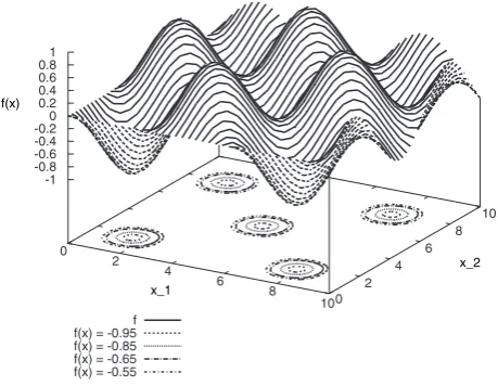
If choosing for instancee¼0.3, the set of approximate solutionsMQ,econsists of five connected components,

each of them containing one minimizerx

i. Further,

for_{¼(2, 2) an ‘optimal’ archiverAcontains exactly} five solutions, each of them approximating one min-imizerx

i (compare to Fig. 3).

In order to compare the result of the novel approach (i.e. DE_þarchiver), we have chosen to take a multi-start optimization process (using FMINCON of MATLAB, http://www.mathworks.com.) and a random search procedure, both equipped with the archiverArchiveUpdateMQ,eDx. We have not

(21) contains a total of 2000 local minima, but only five of them are contained inMQ,e. Hence, a comparison is

not suitable.

Tables 1 to 3 show some averaged numerical results using the three algorithms and a budget of 12 000 function calls per run. For DE, a population size of 200 has been used together with the rand/1 strategy, and the Fweight factor of the DE was set to 0.9 in

all cases. Table 1 shows the number of connected components detected by each method. Here, DE clearly outperforms the two other methods. This is important to note since the maintainance of diversity is an important issue when considering approximate solutions as motivated in section 1. Tables 2 and 3 are dedicated to the (local) convergence behaviour of the archive entries. Since MQ consists of five different

solutions, the following values have been chosen to be used for a comparison (note that both setsAfinal

andMQare finite, and hence, the operators min and

max can be used)

dist_ðAfinal,MQÞ ¼ max a2Afinal

min

i¼1,..._,5kax

ik ð23Þ

that is, the maximal distance from an archive entry ofAfinaltoMQ, and the Hausdorff distance

dHðAfinal,MQÞ ¼maxðdistðAfinal,MQÞ,distðMQ,AfinalÞÞ

ð24_Þ where

dist_ðMQ,AfinalÞ ¼ max

i¼1,::_,5amin₂Afinalk x

i ak ð25Þ

Surprisingly, DE can compete with the FMINCON

solver when consideringdist(Afinal,MQ) in this

exam-ple (and is even better in the mean), and is by far the best when considering the Hausdorff distance. The latter is strongly connected to the result in Table 1.

Since all the local minima of (21) within MQ,e

are also global minima it could be argued that the problem is equal to a ‘classical’ single-objective opti-mization problem. To investigate if DE is also able to pull the population toward local optima withinMQ,e,

which are not global ones we consider the following variation of problem (21)

fðxÞ ¼

sin_ðx1Þsinðx2Þ 0:15 ifkðx1,x2Þk₁4

sinðx1Þsinðx2Þ if5kðx1,x2Þk₁410

sin_ðx1Þsinðx2Þ þ1 otherwise

8 > <

> :

ð26_Þ

f f(x) = -0.95 f(x) = -0.85 f(x) = -0.65 f(x) = -0.55 0

2 4

6 8

10 x_1

0 2

4 6

8 10

x_2 -1

-0.8 -0.6 -0.4 -0.2 0 0.2 0.4 0.6 0.8 1

f(x)

Fig. 3 Surface and contour plot of objective (21) within the ranges [0, 10]2and the setsMQ,efor different

values ofe(the circles around the minimizersx i

indicate the boundaries ofMQ,e)

Table 2 Distance from the archive obtained with each method to the optima set. Minimum, maximum, and average values are over 100 independent runs with at least one compo-nent reached. The best values are emphasized in boldface

Dist(Afinal,MQ)

Method Min Mean Max

Random search 1.54819e-01 7.95134e-01 3.30567eþ00

Multistart (fmincon) 7.18079e-07 1.48833e-01 3.46062eþ00

Using DE 4.17808e-03 2.96775e-02 3.96064e-01

Table 3 Hausdorff distance between the archive obtained with each method and the optima set. Minimum, maximum, and average values are over 100 independent runs with at least one component reached. The best values are emphasized in boldface

Hausdorff

Method Min Mean Max

Random search 6.76238e-01 5.20366eþ00 9.32016eþ00

Multistart (fmincon) 4.44283eþ00 6.28666eþ00 1.12152eþ01

Using DE 4.17808e-03 2.51149e-01 4.44260eþ00

Table 1 Number of components found by each method. Minimum, maximum, and average values are over 100 independent runs

Number of components found

Method Min Mean Max

Random search 1 2.92 5

Multistart (fmincon) 0 1.79 4

Using DE 4 4.97 5

For Q_¼[0, 200][0, 200] and e¼0.3 M_Q,e contains

the same five local minimax

1 tox5, but onlyx1 is a

global solution. Table 4 shows a comparison of the components found by each algorithm. The new strategy outperforms the other methods in terms of finding both the global minimum as well as the local minima withinMQ,e. Hence, it can be argued that DE

is in this case also able to pull the population toward locally optimal solutions.

Summarizing, it can be said that the new strategy (DEþArchiveUpdateMQ,eDx) is efficient in

approxi-mating all the local minima of MQ,e(and only them

in this case). However, it has to be noted that the result (i.e. the set of entries which are kept in the archive) highly depends on the choice of e and which isad hocunclear for this (and in principle for any other) academic model.

5.2 Example B

The next academic function under consideration is (compare to Example 3.2)

f :_R2_!R

f _ðx_{Þ ¼}x₁2_þx₂2 ð27Þ

Figure 4 shows some numerical results for the two different archiving strategies and different discretiza-tions. In all cases, e¼1 has been chosen and

N_¼100 000 randomly chosen points out of the domain Q_¼[2, 2]2 have been inserted into the archivers. Figure 4 (a) shows the result of

ArchiveUpdateMQ,e, where the final archiveAfinal

con-sists of the numerically intractable amount of 16 607 elements. Figure 4 (b) shows a result of the archiver

ArchiveUpdateMQ,eDx using ¼(0.1, 0.1) leading

to 175 archive entries. Though this is, unlike the first result, a tractable number of elements, similar small values of the entries of _{can quickly lead} to similar problems when increasing the number

of parameters. A possible remedy could be (if possi-ble) to assign different values for the entries _i according to their significance. Figure 4 (c) shows a result of ArchiveUpdateMQ,eDx for ¼(0.1, 1).

Hereby, it is assumed that a change inx1is relatively

important (and results with even small changes inx1

have to be stored) while a change in parameterx2is

not of relevance (or not as relevant as a change inx1).

Accordingly, the result in Fig. 4 (c) resembles more a 1D set than a 2D set (as it is the case for MQ,e).

Proceeding in a similar manner, the ‘dimension’ of

MQ,e (and hence the number of elements in the

−2 −1.5 −1 −0.5 0 0.5 1 1.5 2

−2 −1.5 −1 −0.5

0

0.5

1

1.5 2

x1 x 2

(a)

ArchiveU pdateM

,|Af inal|= 16,607

−2 −1.5 −1 −0.5 0 0.5 1 1.5 2

−2 −1.5 −1 −0.5 0 0.5 1 1.5 2

x₁ x 2

(b)

ArchiveU pdateM Dx,∆=(0.1,0.1),

|Af inal|= 175

|Af inal|= 19

−2 −1.5 −1 −0.5 0 0.5 1 1.5 2

−2 −1.5 −1 −0.5

0

0.5

1

1.5 2

x₁ x 2

(c)

ArchiveU pdateM Dx,∆=(0.1,1),

Fig. 4 Numerical results for SOP (27) using dif-ferent archiver and difdif-ferent discretization parameters

Table 4 Number of components found by each method (minimum, maximum and average values are over 100 runs, each run with a budget of 12 000 function evaluations) and percentage of runs that reached the compo-nent corresponding to the global optima. The best values are emphasized in boldface

Number of

components Percentage of runs

reaching the optimal component

Method Min Mean Max

Random search 1 2.73 5 77

Multi-start (fmincon) 0 1.9 5 40

archive) can be reduced in any order according to the problem and the computational limitations: if, in the extreme case, the value _{i¼biai is chosen,} whereaiandbiare the bounds for parameterxi, then

the archiver makes no distinction with respect toxi,

and hence, the ‘dimension’ of the outcome set obtained byArchiveUpdateMQ,eDxis indeed reduced.

5.3 Transfer from earth to apophis

In addition to the previous academic examples, three interplanetary trajectory design problems are consid-ered in the following.

The peculiarity of all problems (as well as other problems related to space mission design) is that: the local minima are – similar to Rosenbrock’s famous banana function – typically located in long, narrow valleys, often flat in one particular direction; there are multiple local minima grouped in clusters with a funnel structure [24]. Hence, such problems are typically (i) hard to solve and (ii) the approxima-tion ofMQ,eby usingArchiveUpdateMQ,eDxcan

con-tain a tremendous number of archive entries for small or even moderate values of _{. To avoid this and} to obtain a meaningful approximation of MQ,e, the

authors of this article have proceeded as described in the previous subsection: the domain was divided into ‘significant’ and ‘insignificant’ parameters. For the significant parameters (launch date, initial veloc-ity, and time of flights), the discretization parameter _{i¼(biai)/0.01, i.e. 1 per cent of the given range} [ai,bi], has been chosen, and for the insignificant

parameters (angles, k2) the value j¼(bjaj)/0.1

has been chosen.

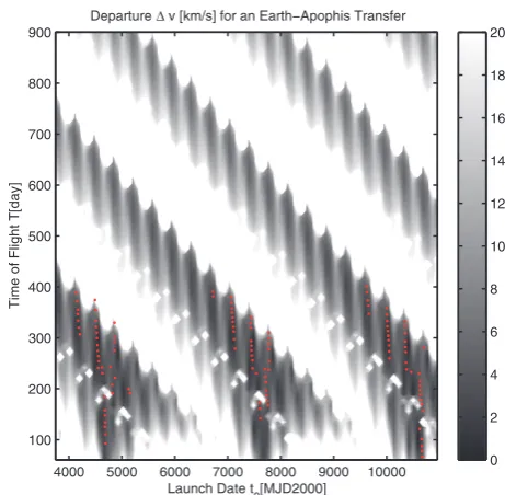
The first example is an apparently simple transfer from the Earth to the asteroid Apophis. The transfer is performed by applying a change of velocity at depar-ture, or_{v, to leave the Earth, and a change of velocity} at Apophis to rendezvous with the asteroid. The cost function is the sum of the modula of the two velocity variations. Due to the similarity of the orbital ele-ments of the two celestial bodies, there exist many local minima corresponding to many possible ways to reach Apophis. The cost function depends on the launch date and transfer time. Here, both parameters have been chosen to be significant and a wide range of values was chosen for both parameters (about 7000 days for the launch date and 800 for the transfer time). Over such a wide range of values, identifying the global minimum is a challenge. Figure 5 shows the level curves of the objective function. Darker areas correspond to lower values of the total_{v. In Fig. 1,} one can observe a large number of local minima with the associated long narrow neighbourhood men-tioned before. The minima are grouped and the

clusters are distributed along the launch-date axis with a certain periodicity. Each cluster, or group of minima, belongs to a different funnel.

For this kind of problems, although the identifica-tion of the global minimum is useful, it is also not sufficient to design a mission. Decision makers require other two pieces of information: given an optimal launch date and transfer time, alternative launch dates and transfer times with similar cost are required as back up options, for each locally optimal launch date and transfer time all transfer solutions in a close neighbourhood of the local minimum are required. The set of solutions that are in a neighbour-hood of the local minimum and at a distanceefrom it in the image space, form the so-called launch window. A wide launch window means a flexible mis-sion that can accommodate delays and contingen-cies. The set of local minima with similar cost represents multiple launch opportunities: a mission with multiple launch opportunities offers a higher degree of robustness and flexibility.

The dots in Fig. 5 are the solutions collected by the archiving strategy usinge¼0.5 [km/s], after n¼1e7 function evaluations of Differential Evolution, with a population size of 100, F¼0.9, and CR¼1. The

archiving procedure correctly identified the most interesting launch opportunities (lowest _{v) with} their associated local neighbourhood. Therefore, in this case, the decision maker is offered with three groups of launch opportunities and for each one

Launch Date t₀[MJD2000]

Time of Flight T[day]

Departure∆ v [km/s] for an Earth−Apophis Transfer

4000 5000 6000 7000 8000 9000 10000 100

200 300 400 500 600 700 800 900

0 2 4 6 8 10 12 14 16 18 20

multiple launch windows with transfer times ranging from less that 100 days to over 400 days. All the col-lected solutions have a total_{vat an}edistance from the best solution, therefore, they are all admissible. In fact, the value e is easily set a priori based on mission constraint on the available _{v budget.} Note that the best known solution for this problem is included in the archive.

6 THE ROSETTA CASE

This second case study is a multigravity assist trajec-tory from the Earth to the comet 67P/Churyumov– Gerasimenko following the gravity assist sequence that was planned for the spacecraft Rosetta: Earth– Earth–Mars–Earth–Earth–Comet. This mission was initially scheduled for launch on an Ariane 5 launcher. However, due to a failure in the previous launch, the mission had to be rescheduled. Rescheduling a mission with such a complex sequence of gravity assist manoeuvres is not an easy matter. Therefore, for this type of mission, it is desir-able to generate multiple transfer options since the start of the mission design process. The trajectory model considered here is the one described in refer-ences [1,2]. A deep space maneuver is allowed along the transfer arc from one planet to the other accord-ing to the model presented in references [1,24]. The objective is the sum of all the deep space manoeuvres plus the initial_{v0at departure and the finalvf to} rendezvous with the comet. The search space for this problem has 22 dimensions and cannot be graphi-cally completely represented. An analysis of this search space can be found in reference [24]. Even in this case the local minima are grouped in multiple funnels, for each funnel, the analysis in reference [24], revealed a high number of local minima irregu-larly distributed.

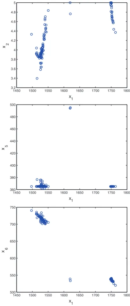
Figure 6 shows three projections of the final archive

Afinalof one run of the algorithm described in section

3 fore¼0.5 [km/s] and as described above. A_final consists of a total of 122 elements and contains an approximation of the best known solution 20 P1

withf(P1)&1.34 [km/s] [2] as well as othere -approx-imate solutions ofP1within three connected

compo-nents. The three local optima within the components are shown in Table 5. The clusters in Figure 6 corre-spond to the funnel structures identified in reference [24]. As already mentioned in section 1, the DM is offered (at least) two more options in addition to the best known trajectory. Also, the number of archive entries is tractable since it does not slow down the computational cost significantly. If, hypo-thetically, for unified small values of_{ithree points} per coordinate direction and connected component

would have been required for the approximation (which is much less than shown in Fig. 6), this would have led to a total of 3322&₁₀11 _archive

entries, which would certainly not have been realizable.

1450 1500 1550 1600 1650 1700 1750 1800 3.2

3.4 3.6 3.8 4 4.2 4.4 4.6 4.8 5

x₁ x 2

1450 1500 1550 1600 1650 1700 1750 1800 360

380 400 420 440 460 480 500

x₁ x 5

1450 1500 1550 1600 1650 1700 1750 1800 500

550 600 650 700 750

x₁ x 6

Fig. 6 Numerical results for the Rosetta case. Hereby,

x1 denotes the value of the launch date

(MJD2000),x2denotes the initial velocity (km/

s),x5denotes the time of flight for the first arc of

the trajectory (d), andx6the time of flight for the

7 THE CASSINI CASE

The Cassini case is a multigravity assist trajectory from the Earth to Saturn following the sequence Earth–Venus–Venus–Earth–Jupiter–Saturn (EVVEJS). Even in this case, a deep space manoeuvre is allowed along the transfer arc from one planet to the other according to the model presented in reference [1, 24]. The objective is the sum of all the deep space manoeuvres plus the initial _{v0 at departure} and the final _{vf at arrival at Saturn. This model} reproduces the actual Cassini–Huygens mission that was launched in 1997 and successfully entered into orbit around Saturn in 2004. Unlike the Rosetta case, the current hypothesis from previous analyses is that there is only one principal funnel and that the minima are nested in very narrow valleys. Figure 7 shows a final archive Afinal (with jAfinalj ¼635)

obtained from this model using the same values for eandas for the Rosetta case.

From Fig. 7, one can see one main cluster with the solutions distributed in two connected groups. In the x1x6 and x1x5 planes, i.e. launch time,

time of flight of the first transfer arc, time of flight of the second transfer arc, one can notice that the solutions are aligned along particular directions, revealing a narrow valley structure. In the x1x2

plane, the solutions are much more scattered, although still two main groups can be identified (for further details on this particular problem, please refer to reference[24].

Therefore, also in this case, the archiving procedure seems to have correctly captured the distribution of the minima, providing information on the structure of the problem. The DM is offered a variety of options which are all admissible, because e is the

−8203 −810 −800 −790 −780 −770 −760 3.5

4 4.5

x₁ x 2

−820 −810 −800 −790 −780 −770 −760 140

150 160 170 180 190 200 210

x₁ x 5

−820 −810 −800 −790 −780 −770 −760 410

420 430 440 450 460 470 480

x₁ x6

Fig. 7 Numerical results for the Cassini case. Hereby,

x1 denotes the value of the launch date

(MJD2000), x2 denotes the initial velocity

(km/s), x5 denotes the time of flight for the

first arc of the trajectory (d), andx6the time of

flight for the second arc of the trajectory (d)

Table 5 The three local solutions Pi,i¼1, 2, 3, from

the three connected components shown in Fig. 6

Variable Units P1 P2 P3

x1 MJD2000 1.542Eþ03 1.748Eþ03 1.620Eþ03

x2 km/s 4.443Eþ00 5.000Eþ00 5.000Eþ00

x3 n/a 9.881E-01 5.146E-01 9.613E-01

x4 n/a 5.623E-01 2.958E-01 5.000E-01

x5 Days 3.652Eþ02 3.652Eþ02 4.940Eþ02

x6 Days 7.082Eþ02 5.391Eþ02 5.389Eþ02

x7 Days 2.574Eþ02 6.810Eþ02 6.811Eþ02

x8 Days 7.304Eþ02 6.307Eþ02 6.309Eþ02

x9 Days 1.850Eþ03 1.818Eþ03 1.813Eþ03

x10 n/a 3.178E-01 5.496E-01 4.151E-01

x11 n/a 8.097E-01 1.088E-01 9.516E-02

x12 n/a 1.361E-01 4.308E-01 3.963E-01

x13 n/a 6.566E-01 2.713E-01 4.703E-02

x14 n/a 4.375E-01 4.908E-01 4.876E-01

x15 n/a 2.986Eþ00 2.374Eþ00 1.699Eþ00

x16 n/a 1.050Eþ00 1.050Eþ00 1.050Eþ00

x17 n/a 3.202Eþ00 3.326Eþ00 3.338Eþ00

x18 n/a 1.050Eþ00 1.050Eþ00 1.050Eþ00

x19 rad 3.273Eþ00 3.122Eþ00 3.361Eþ00

x20 rad 2.187E-01 4.443E-01 4.423E-01

x21 rad 3.135Eþ00 2.556Eþ00 2.560Eþ00

x22 rad 3.554Eþ00 3.656Eþ00 3.656Eþ00

quantification of the available_{vbudget and all differ} at least by the value of_.

8 CONCLUSIONS AND FUTURE WORK

In this article, the problem of computing the setMQ,e

of e-approximate solutions of a scalar optimization problem with a focus on local minima has been addressed. For this, two archiving strategies have been proposed, one which captures alle-approximate solutions out of the obtained data, and another one which uses a certain discretization strategy. Since the dimension of MQ,e is typicallyn, where n is the

number of parameters involved in the model, the first archiver is mainly of theoretical interest, and required a suitable discretization. The strategy used in the second archiver is designed to focus on the local minima within MQ,e. However, the outcome

of the archiver is crucially dependent on the choice of the discretization parameter _2Rn

þ which has

hence to be chosen problem dependent. Since the ‘optimal’ choice of this parameter may be ad hoc

unclear, or intuitive choices may lead to a numeri-cally untractable number of archive entries, one way to reduce the elements in the archive has been dis-cussed which has an analogue effect as the reduction of the dimension of the set of interest and which allows for the efficient treatment of higher dimen-sional problems. Finally, the efficiency of the search strategy (DE together with the new archiver) has been shown on some benchmark functions and its useful-ness has been illustrated showing several models related to space mission design.

As part of our future work, an adaptive choice of would be of particular interest for both theoretical and practical considerations: such an adaptation could for instance be used to explore the neighbour-hood of a locallye-approximate solution withinM_Q,

e

since this set is very important to quantify its robust-ness. Finally, open branches of research can be found when interleaving the archive with the generator heu-ristic (DE, PSO, etc.) as a matter of feedback into its main population.

FUNDING

C. A. Coello Coello acknowledges support from CONACyT project no. 128554. Adriana Lara acknowl-edges support from ESFM-IPN and CONACyT to pursue graduate studies at the Computer Science Department of CINVESTAV-IPN. M. Vasile acknowl-edges support from CONACyT project no. 103570.

ß_{Authors 2011}

REFERENCES

1 Vasile, M. and De Pascale, P. Preliminary design of multiple gravity-assist trajectories. J. Spacecraft Rockets, 2006,43(4), 5–22.

2 Vasile, M., Minisci, E.,andLocatelli, M.A dynamical system perspective on evolutionary heuristics applied to space trajectory optimization problems. In Proceedings of the 2009 IEEE Congress on

Evolutionary computation (CEC 2009), Trondheim, 18–21 May 2009, pp. 2340–2347.

3 Olds, A. D., Kluever, C. A., and Cupples, M. L.

Interplanetary mission design using differential evolution. J. Spacecraft Rockets, 2007, 44(5), 1060–1070.

4 Peng, L., Wang, Y. Z., Dai, G. M., Chang, Y. M.,and

Chen, F. J. Optimization of the Earth-Moon low energy transfer with differential evolution based on uniform design. In Proceedings of the 2010 IEEE Congress onEvolutionary computation (CEC 2010), Barcelona, 18–23 July 2010, pp. 1–8.

5 Schu¨tze, O., Coello Coello, C. A.,andTalbi, E.-G.

Approximating thee-efficient set of an MOP with sto-chastic search algorithms. In Mexican International Conference on Artificial intelligence (MICAI 2007)

(Eds A. Gelbukh and A. F. Kuri Morales), Agnascaliontes, Mexico, 4–10 November 2007, pp. 128–138 (Springer-Verlag, Berlin/Heidelberg).

6 Schu¨tze, O., Coello Coello, C. A., Tantar, E., and

Talbi, E.-G. Computing finite size representations of the set of approximate solutions of an mop with stochastic search algorithms. In Proceedings of the 10th annual conference onGenetic and evolutionary computation (GECCO 2008), Atlanta, Georgia, USA, 12–16 July 2008, pp. 713–720 (ACM, New York, USA).

7 Schu¨tze, O., Vasile, M., and Coello Coello, C. A.

Approximate solutions in space mission design. In Proceedings of the 10th International Conference on Parallel problem solving from nature (PPSN 2008), Dortmund, Germany, 13–17 September 2008, pp. 805–814.

8 Schu¨tze, O., Lara, A., Coello Coello, C. A., and

Vasile, M. Computing approximate solutions of scalar optimisation problems and applications in spacemission design. In Proceedings of the 2010 IEEE Congress on Evolutionary computation (CEC ’10), Barcelona, Spain, 18–23 July 2010, pp. 1654–1661.

9 Li, J.-P., Balazs, M. E., Parks, G. T.,andClarkson, P. J. A species conserving genetic algorithmformulti-modal function optimization. Evolut. Comput., 2002,10(3), 207–234.

10 Li, X. Adaptively choosing neighbourhood bests using species in a particle swarm optimizer for multimodal function optimization. In Proceedings of the Conference on Genetic and evolutionary computation (GECCO ’04), Seatle, USA, 1 June 2004, pp. 105–116 (Springer-Verlag).

onEvolutionary computation (CEC ’06), Vancouver, Canada, 16–21 July 2006, pp. 816–822.

12 Zhang, J., Huang, D.-S.,andLiu, K.-H. Multi-sub-swarm particle Multi-sub-swarm optimization algorithm for multimodal function optimization. In Proceedings of the 2007 IEEE Congress onEvolutionary compu-tation (CEC ’07), Singapore, 25–28 September 2007, pp. 3215–3220.

13 Brits, R., Engelbrecht, A. P.,andvan den Bergh, F.

Locating multiple optima using particle swarm opti-mization. App. Math. Comput., 2007, 189(2), 1859–1883.

14 Vitela, J. E.andCastan˜ os, O.A real-coded niching memetic algorithm for continuous multimodal func-tion optimizafunc-tion. In IEEE Congress onEvolutionary computation (CEC 2008), Hong Kong, China, 1–6 June, 2008, pp. 2170–2177.

15 Passaro, A. and Starita, A. Particle swarm optimization for multimodal functions: a clustering approach.J. Artif. Evol. Appl., 2008,8(2), 1–15.

16 Li, X.Niching without niching parameters: Particle swarm optimization using a ring topology. IEEE Trans. Evolut. Comput., February 2010, 14(1), 150–169.

17 Saha, A. and Deb, K. A bi-criterion approach to multimodal optimization: Self-adaptive approach. In Simulated evolution and learning (Eds K. Deb et al.), vol. 6457, Lecture Notes in Computer

Science, 2010, pp. 95–104 (Springer, Berlin/ Heidelberg).

18 Vasile, M. and Locatelli, M. A hybrid multiagent approach for global trajectory optimization.

J. Global Optim., 2009,44(4), 461–479.

19 Laumanns, M., Thiele, L., Deb, K.,andZitzler, E.

Combining convergence and diversity in evolutio-narymultiobjective optimization. Evolut. Comput., 2002,10(3), 263–282.

20 Schu¨tze, O., Coello Coello, C. A., Tantar, E., and

Talbi, E.-G.Computing a finite size representation of the set of approximate solutions of an MOP. INRIA Research Report, Technical Report 6492, 2008.

21 Schu¨tze, O., Laumanns, M., Coello Coello, C. A., Dellnitz, M.,andTalbi, E.-G.Convergence of stochas-tic search algorithms to finite size Pareto set approx-imations.J. Global Optim., 2008,41(4), 559–577.

22 Schu¨tze, O., Laumanns, M., Tantar, E., Coello Coello, C. A.,andTalbi, E.-G.Computing gap free Pareto front approximations with stochastic search algorithms.Evolut. Comput., 2010,18(1), 65–96.

23 Price, K. V., Storn, R. M., and Lampinen, J. A. Differential evolution: a practical approach to global optimization, 2005 (Springer Verlag).

24 Vasile, M., Minisci, E., andLocatelli, M. An infla-tionary differential evolution algorithm for space tra-jectory optimization. IEEE Trans. Evolut. Comput.