ABSTRACT
BALASUBRAMANIAN, NISHANTH. ScalaMemAnalysis: A Compositional Approach to Cache Analysis of Compressed Memory Traces. (Under the direction of Dr. Frank Mueller.)
Cache simulators use lengthy traces files and maintain/update a complete cache state per trace. Analyzing these trace files can be a time-consuming and cumbersome process.
In previous work, a tool (ScalaMemTrace) was developed that uses binary instrumentation to gener-ate memory traces and to compress these traces. We exploit these compressed traces to accelergener-ate cache analysis in ScalaMemAnalysis (SMA) for a uni-processor system. Instead of a complete simulation, we utilize a context-based reuse distance, which tracks the number of arrays that can fit within the cache. This context information is kept at each loop level for cache analysis across all loop and changes with the composition of additional context information at each loop nesting.
© Copyright 2014 by Nishanth Balasubramanian
ScalaMemAnalysis: A Compositional Approach to Cache Analysis of Compressed Memory Traces
by
Nishanth Balasubramanian
A thesis submitted to the Graduate Faculty of North Carolina State University
in partial fulfillment of the requirements for the Degree of
Master of Science
Computer Science
Raleigh, North Carolina
2014
APPROVED BY:
Dr. William Enck Dr. David Thuente
DEDICATION
BIOGRAPHY
ACKNOWLEDGEMENTS
TABLE OF CONTENTS
LIST OF FIGURES . . . vii
Chapter 1 Introduction . . . 1
1.1 Hypothesis . . . 2
1.2 Contributions . . . 2
Chapter 2 ScalaMemTrace . . . 4
2.1 Overview . . . 4
2.2 Redesign . . . 5
Chapter 3 ScalaMemAnalysis Design . . . 7
3.1 Assumptions and Definitions . . . 7
3.2 PRSD Tree Structure . . . 9
3.3 Context-Based Reuse Distance . . . 9
3.4 Algorithms for Context Composition . . . 10
Chapter 4 ScalaMemAnalysis Implementation . . . 15
4.1 Assumptions . . . 15
4.2 Array Classifiers . . . 15
4.3 Pure Conflicts . . . 16
4.4 Partial Conflicts . . . 17
4.5 Handling Varying Strides . . . 19
4.6 Forward Stride Analysis . . . 20
4.7 Handling Varying Loop Depth . . . 21
4.8 Classifier Modifiers . . . 21
4.9 Tracking Cache Capacity and Associativity . . . 22
4.10 Special Cases . . . 22
Chapter 5 Experimentation Results . . . 25
5.1 Test Framework . . . 25
5.2 Timing . . . 25
5.3 Accuracy . . . 28
5.4 Case Study . . . 32
Chapter 6 Related Work . . . 39
Chapter 7 Future Work. . . 40
Chapter 8 Conclusion . . . 41
References . . . 42
Appendix . . . 45
LIST OF FIGURES
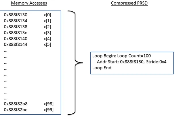
Figure 1.1 Regularly Strided Memory Access compressed to PRSD . . . 3
Figure 2.1 ScalaMemTrace compression . . . 5
Figure 2.2 Nested loop compression by ScalaMemTrace . . . 6
Figure 3.1 Data Flow of Cache Simulator . . . 8
Figure 3.2 PRSD Tree Structure . . . 9
Figure 3.3 Example for Population of Left and Right Context . . . 10
Figure 3.4 Internal Composition Between Left and Right Context . . . 12
Figure 3.5 Composition between Outer Loop and Inner Loop Context . . . 13
Figure 4.1 Pure Conflict Case . . . 17
Figure 4.2 Four Partial Conflict Cases . . . 18
Figure 4.3 Partial Conflict Analysis Example . . . 19
Figure 4.4 Example of Intra-Loop Analysis . . . 23
Figure 5.1 Execution Time for Varying Loop Nest Levels . . . 26
Figure 5.2 Execution Time for Matrix Multiplication . . . 26
Figure 5.3 Execution Time for Matrix Multiplication with Blocking . . . 27
Figure 5.4 Execution Time for SPEC Test Cases . . . 27
Figure 5.5 Execution Time for NAS Test Cases . . . 28
Figure 5.6 Memory Latency for Nested Loops . . . 29
Figure 5.7 Memory Latency for Matrix Multiplication . . . 29
Figure 5.8 Percent Miss Difference for Matrix Multiplication . . . 30
Figure 5.9 Percent Miss Rate Difference for Matrix Multiplication . . . 31
Figure 5.10 Memory Latency for Matrix Multiplication with Blocking . . . 32
Figure 5.11 Percent Miss Difference for Matrix Multiplication with Blocking . . . 33
Figure 5.12 Percent Miss Rate Difference Matrix Multiplication with Blocking . . . 34
Figure 5.13 Memory Latency for SPEC Benchmark Suite . . . 34
Figure 5.14 Percent Miss Difference for SPEC Benchmark Suite . . . 35
Figure 5.15 Percent Miss Rate Difference for SPEC Benchmark Suite . . . 35
Figure 5.16 Memory Latency for NAS Benchmark Suite . . . 36
Figure 5.17 Percent Miss Difference for NAS Benchmark Suite . . . 36
Figure 5.18 Percent Miss Rate Difference for NAS Benchmark Suite . . . 37
Figure 5.19 Timing results for Matrix Multiplication with Blocking . . . 37
Chapter 1
Introduction
Applications generally have millions of accesses to data in memory. Part of this data is stored in a cache so as to provide fast access to memory references that take advantage of spatial and temporal locality. However, this may not always be the case. Cache performance makes a huge impact on the runtime of an application. Thus, taking advantage of the cache by trying to keep data frequently by the application in cache would be the ideal situation. Identifying these data structures may be a difficult task for a user. One approach would be to use memory traces and a cache simulator to determine the cache performance. Cache simulators generally use full length traces, which contain information such as addresses ac-cessed and the type of access, and maintain a complete cache state, which is updated per memory access to obtain data on the hits and misses within the cache. Such trace files usually span Gigabytes of data and the data obtained from the cache simulator can only predict the current performance of the cache for the individual memory accesses. Analyzing these huge trace files along with the cache simulator data can be a time-consuming and cumbersome process.
In previous work, a tool (ScalaMemTrace) was developed which uses binary instrumentation [19] to generate memory traces and to compress these traces to near constant size by identifying and grouping similar memory access patterns into single entities.
There has been some previous work on cache analysis [18] where compressed traces have been used. But their approach does not consider the problem of identifying data structures causing cache misses. Our work allows the user to identify arrays that miss often within the cache and provides cache statistics at loop level granularity to better understand the reason behind the cache performance of an application. There are some compression techniques which have reduced I/O when passed to a trace-driven sim-ulator [17, 16]. However, the processing of theses traces before simulation does not provide a significant speedup in execution time.
1.1
Hypothesis
We hypothesize that with cache analysis of compressed traces, we can significantly reduce the cost of determining cache behavior time while achieving close resemblance in accuracy of predicated cache behavior compared to conventional trace-based cache simulation.
1.2
Contributions
ScalaMemAnalysis (SMA) focuses on using the compressed traces topredict the performance of the cache for a uni-processor system by analysisinstead of simulation. The memory accesses within a loop have regular strides and each group of these accesses can be considered as an array as show in Figure 1.1. Our cache analysis algorithm is based on the concept of reuse distance [8], a metric to denote the number of distinct memory accesses between two identical memory accesses. We use a context-based reuse distance and create a context to keep track of the number of arrays that can fit within the cache. This context information is kept per loop and is used to predict the cache performance. Each loop is analyzed at every loop nesting level to determine the cache performance per loop level and performance changes with the composition of additional context information at each loop nesting. This information also provides an insight to the user as to which arrays/loops at which level degrade the performance of the cache.
There has been previous work on compressing traces and simulating cache performance [15, 17, 16], but this is the first framework to supportcompositionalanalysis to determine cache performance, to the best of our knowledge.
Our experimental results indicate that the accuracy of our method close to our reference trace-driven simulator and results in a near constant execution time which is a significant speedup over Dinero IV and allows unprecedented scalability of cache simulations/analysis.
Chapter 2
ScalaMemTrace
ScalaMemTrace [4] is a novel technique for collecting memory traces in a scalable manner. It performs a scalable trace compression on-the-fly. The tool generates near-constant size compressed trace files that preserve the temporal order of accesses.
2.1
Overview
A RSD (Regular section descriptor) [11] describes the memory being accessed. It contains information such as the address accessed. address stride and access type(read/write). A PRSD (Power RSD) contains information about the loop enclosing the RSDs. It contains information such as the loop count and the number of RSDs present in the loop and address pattern meta-data (strides). An example PRSD and RSD can found in Section A.
The memory trace compression scheme is based on the PRSD abstraction [20] which preserves the order of memory references and generalizes memory access patterns across threads. An example of a PRSD generation is shown in Figure 1.1.
A binary instrumentation tool, Pin [19], is used to extract memory accesses (loads and stores) from an application and the output is fed to a compressor module, which recognizes repetitive behavior of memory access patterns on-the-fly and produces a compressed trace file.
Each new entry is added to the list of memory traces. Each memory access has a unique signature attached to it, which is computed by using a stack-walk. The unique signature generation is a necessary step since a single instruction can perform multiple memory operations. The stackwalk generates a series of program counter values, which are XORed to produce a unique signature for each memory trace. This is the criteria for recognizing memory access patterns and compressing them. The compressed memory trace contains RSDs and PRSDs, which represent memory accesses and loop nests, respectively.
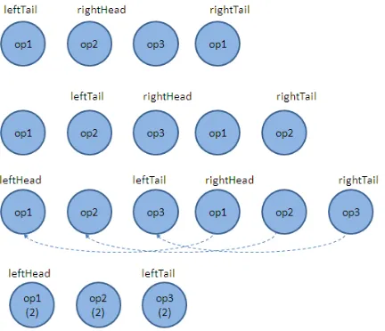
Figure 2.1: ScalaMemTrace compression
the right tail. A matching node is searched for and marked as left tail. The right tail and left tail are traversed in reverse to find a matching sequence. On finding a matching sequence, the right portion is merged with the left portion and the RSD count is incremented. This process repeats for subsequent sequences of op1, op2 and op3 until the pattern disappears.
2.2
Redesign
The objective of ScalaMemTrace was to generate an accurate compression with respect to the count of the number of memory references and their access pattern. Thus, when the compressed trace file was replayed using the replay tool, it generated the same number of references as the original trace file. In certain cases however, the right addresses were not generated since the main criteria used for compression was to ensure matching of signatures. Data structures with different strides at different loop levels, in case of a nested loop, was not accounted for.
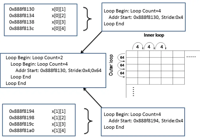
ScalaMemTrace has been redesigned by expanding the data structures to support multi-level stride information. The criteria for a pattern match now includes matching stride data between traces. Thus, only traces with a match in sign and stride will be added to expand a PRSD. When the stride changes, a new PRSD is created. The compression then occurs between these levels of PRSDs to create a nested PRSD.
matching PRSD lengths and RSD strides, they can be compressed to a nested PRSD with a second level stride of 0x64 as shown in the figure. The new stride is calculated as the difference between the two start addresses of the two RSDs before the nested PRSD compression.
Chapter 3
ScalaMemAnalysis Design
Let us discuss the idea of cache performance analysis instead of simulation. It includes a description of the context-based reuse distance along with algorithms to facilitate cache analysis. A more thorough description will be given in Section 4.
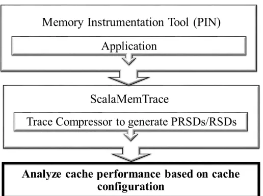
Figure 3.1 shows a high-level overview of the blocks involved in the process. An application is first executed inside a binary instrumentation tool, which captures all memory references, i.e., all loads and stores to memory. The instrumentation is modified to also perform a stack walk for each memory ref-erence to provide a unique signature per memory refref-erence. The output of the tool is in a format that contains information such as the address, type and signature of each memory reference . This infor-mation is piped into the ScalaMemTrace tool, which compresses the memory references by identifying patterns based on signature and calculated stride information to generate RSDs and PRSDs. The gen-erated compressed trace is processed by our cache analyzer along with the specified cache parameters. This allows us to perform a detailed analysis of the how the different data structures preform at different loop levels in terms of their cache behavior.
3.1
Assumptions and Definitions
Three types of misses which are commonly distinguished in a uni-processor cache. They are compulsory, capacity and conflict misses [23]. Compulsory misses are those misses caused by the first reference to a location in memory. Capacity misses are those misses that occur regardless of associativity or block size, solely due to the finite size of the cache. Conflict misses are those misses which occur due to mapping of multiple cache lines to the same cache set and could have been avoided with a higher associativity or better mapping.
Figure 3.1: Data Flow of Cache Simulator
with our analysis would require an additional overhead in data structures and computation which is undesirable.
Our analysis accepts in three cache configuration parameters, namely the cache size, the block size and the cache associativity.
When we discuss ”arrays” present in the cache, arrays represent a strided RSD within a loop. The loop length multiplied by the stride gives the total number of bytes within the array. The reference to a wayin cache refers to an entire column of blocks in the cache i.e. set 0 to setnwhere n = (total blocks / associativity).
The context information can be defined as follows:
Context={a,b,c..,x:SC≤CC} (3.1) where
a,b..= arrays present in the cache context
SC = aggregate size of all array blocks in the cache context
CC= cache capacity
allocation policies as it is not necessary for our analysis since we do not maintain a complete cache state, such as trace-driven simulator would.
3.2
PRSD Tree Structure
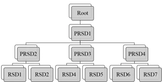
The compressed trace file contains PRSDs, which are transformed into a tree as shown in Figure 3.2. The blocks markedPRSDare the loop heads indicating the accesses below denote a loop. They contain information such as the number of memory accesses in the loop and the loop length. The blocks marked RSDare the actual memory accesses. They contain information such as the address accessed and (for a loop) stride information depending on the nesting level. Each RSD member also has containers to hold cache performance data per loop nest level. Figure 3.2 contains one outer loop, three inner loops with each of the inner loop having two RSDs each. The RSDs will contain strides to indicate the actual memory location referenced between successive iterations.
Figure 3.2: PRSD Tree Structure
3.3
Context-Based Reuse Distance
Each loop head has a left and right context. The left context contains the first set of arrays in the loop bounded by the cache capacity. The right context contains the last set of accesses in the loop bounded by the cache capacity. The right context is ordered from Least Recently Used (LRU) to Most Recently Used (MRU) which is done in order to emulate a Least Recently Used Replacement policy of the cache. This can be modified if required to emulate other replacement policies.
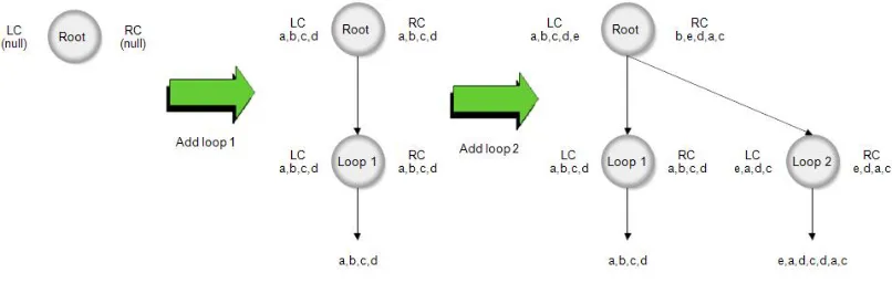
Figure 3.3: Example for Population of Left and Right Context
Figure 3.3 shows an example of how the left context and right contexts are populated with the addition of each loop to the root node. The first loop has four array accesses (a,b,c,d), which are added to the left and right context of the loop. The context information is copied onto the root node since there is no data to compose. When the second loop is added, the left context of the loop is set to the first set of accesses while the right context text is set to the last set of accesses in decreasing order as shown. When this data is composed with the root’s context information, the left and right contexts of the root exhibit the same properties after composition.
3.4
Algorithms for Context Composition
Each PRSD is read sequentially from the compressed trace file and processed when it is read. The tree is initialized with a root node, which is created as a placeholder (Rootin Figure 3.2). It can be considered as a loop head with one iteration.
If the PRSD is a loop head, a new node is created in the tree, and the following data is added as children to this node. The end of the loop is derived from the information present in the loop head.
If the PRSD scanned is a memory access, a child node is added to the current loop head, which contains information such as start address and stride per loop level.
access, the array is compared with the right context to check if the array has already been accessed, i.e., if it is present in the right context. If so, the element is moved up in the list to the MRU position (lines 6-8). If the array has not been accessed previously and is not in the context information, the array is added to the right context if there is no conflicting array and there is enough remaining cache capacity (lines 12-15). If either of the conditions do not hold, the context is modified to make space for the new array and is added to the context (lines 17-18). Classifiers are assigned to the arrays to indicate cache performance at the current loop level.
Algorithm 1AddNewNode (nodeIn f o)
1: Input:A PRSD read from the compressed trace file
2: if(nodeIn f ois a loop head)then
3: Add node as child to current loop head
4: Move pointer to new loop head
5: else .nodeIn f ois a memory access
6: for(i=rightContextCountto 0)do
7: if(nodeIn f o==rc→node[i])then
8: Reorder right context to move node to MRU
9: break
10: end if
11: end for
12: if(nodeIn f onot found in right context)then
13: if(Enough space left in cache)then
14: Add node to right context at MRU
15: Add node to left context
16: else
17: Remove LRU/conflicting array from right context
18: Add node to right context at MRU
19: end if
20: end if
21: end if
22: if(All addresses have been added to loop)then
23: callEndOfLoopComp(currLoopHead,parentLoopHead)
24: end if
This can be defined as follows:
Figure 3.4: Internal Composition Between Left and Right Context
where
X = New array
|X|= Size of array
L= LRU array in context
When all children have been added to the current loop, the loop composition occurs. Before the actual composition, initial pre-processing occurs where the right and left contexts of the current loop are composed to adjust for the effects of conflicting arrays as show in Figure 3.4. This is an essential step to recognize if there are any conflicting arrays in the right context which can affect the arrays in the left context. This composition is done with the same procedure Algorithm 1. In the example, arrayc conflicts withaas per LRU scheme. When the internal composition occurs, it can be seen that arrayb, too, conflicts, indicating that all 3 arrays have conflict misses.
At the loop composition stage, the current loop has been evaluated as an individual loop and its cache performance is predicted. The right and left context of this loop have been populated to indicate the arrays accessed that are still present in cache.
the right context of the parent, which contains the latest accesses seen in the parent loop with the left context of the current loop, which contains the first accesses seen by the loop in order to predict how the current loop affects the cache data in the context of its parent loop. This composition is described in Algorithm 2.
If the parent loop context data has not been initialized, it indicates that the first access under the parent loop is the current loop. Thus, the context data from the current loop are passed onto the parent loop since the parent loop has no context data for composition to occur (lines 3-5).
If the parent loop already has context information, each element of the current loop’s left context is compared to the parent loop’s right context to check if the array has been accessed previously. If the array has any conflicting data in the right context occupying the same cache sets, this array is removed from the right context of the parent loop to make space for the new array in the current loop and the new array is appended to the right context at the end (lines 7-9). If the array did have a previous access, the array is moved to up the right context to maintain ordering (lines 11-12). In both cases, the cache performance counters at the current loop level are suitably adjusted to reflect the new changes. A match in the context indicates the array is already present in cache and the counters for the array will have hits assigned to them. If the array is not present, misses are assigned equal to the number of blocks being accessed in that loop.
A sample composition is shown in Figure 3.5. The first array (arrayb) of the inner loop is found in the outer loop context and is marked as a hit. Then the outer loop is reordered to move arraybto the MRU location. The next array (arraye) is not found in the context. This it is marked as a miss and will be added to the outer loop context.
At the end of the composition, the parent loop’s left context parses more arrays if there is space left in the context (lines 17-18). The right context of the parent and the current loop are composed to ensure that the parent loop retains any older arrays in addition to the new arrays from the current loop within the space constraint by the cache capacity to reflect the latest state of the cache (line 20). This is used for subsequent loops or array accesses.
Algorithm 2EndOfLoopComp(currLoopHead,parentLoopHead)
1: Input:Current loop head being processed and its parent
2: Recompose the left context and right context of the current loop
3: if(parentLoopHeadleft/right context uninitialized)then
4: parentLoopHead→LC=currLoopHead→LC
5: parentLoopHead→RC=currLoopHead→RC
6: else .ComposeCurrentLoopHead→LCandparentLoopHead→RC
7: for(i= 0 tocurrLoopHead→LCCount)do
8: for(j=parentLoopHead→RCCountto 0)do
9: Find the conflicting array (if any) and remove it.
10: end for
11: if(Match found)then
12: ReorderparentLoopHead→RCto move array to MRU
13: else .Match not found
14: Add the new element toparentLoopHead→RC
15: end if
16: end for
17: if(parentLoopHead→le f tContexthas enough space)then
18: Add any new elements toparentLoopHead→LC
19: end if
20: RecomposeparentLoopHead→RCandcurrLoopHead→RC
21: end if
Chapter 4
ScalaMemAnalysis Implementation
This section describes the techniques used to implement the algorithms described in the previous section.
4.1
Assumptions
One of our main assumptions is that SMA only considers arrays that are entirely (not partially) present in the cache. But sometimes, only part of an array may be present in cache. In this case, the array is assumed to benotpresent in the cache. The time and code complexity would increase prohibitively to process and maintain partial arrays in our analysis.
4.2
Array Classifiers
Each array in the context has a category [22] or classifier assigned to it. These classifiers describe the behavior of that array with respect to the current loop being analyzed. These classifiers are modified as we move up the nesting levels and as long as the array remains in context. The contribution to the total misses of the loop under which the array is accessed is based on the classifier it has been assigned during analysis. A list of classifiers and its description are as follows:
• ALWAYS HIT: The array is present in cache resulting in all hits for the current loop.
• FIRST MISS: The array only misses on the first blocks being brought into the cache. The misses do not multiply for outer loops.
• CAP MISS: The capacity misses multiply as the array accesses are repeated by outer loos.
• FIRST HIT: The array only hits on the first blocks and the rest of the accesses are conflict misses.
• ALWAYS MISS: All elements accessed in the array are misses.
Each classifier helps to describe the array behavior, which is helpful during loop composition be-tween inner and outer loop. ALWAYS HIT provides an indication that the array has been brought into the cache previously and will remain in cache. FIRST MISS usually indicates a cold misses when the array is brought into the cache for the first time. Also, this indicates there is enough space in the cache for the array to remain in cache. CAP MISS and CONF MISS occurs when the array cannot remain in cache due to exceeding cache capacity or excessive number of ways in cache, respectively. These misses multiply when traversing up the loop nest. FIRST HIT occurs when an array is present in cache, but for a certain loop the array haspureconflict misses with another array within the same loop. Thus, only each first access of each block of the array result in hit. ALWAYS MISS is assigned to arrays with pureconflict misses. There can be certain other cases, such as an outer loop array is constantly being removed by an inner loop array. This case is covered in section 4.7.
4.3
Pure Conflicts
There are two possible cases of conflicts that can arise between two arrays. The first case is a pure conflict, where the arrays being examined map to the exact same blocks in the cache. The next case is a partial conflict, where only parts of the array overlap. This is discussed in the next subsection.
To detect pure conflicts, i.e. when two arrays completely overlap with each other and constantly replace each other with every iteration, we scan through the right context to match the incoming array for a pure conflict with the arrays present in the context information. When a pure conflict is detected, it indicates that the way in cache is used by the array in the context information. In the next step, the cache associativity is checked to see if there is another way available for the incoming array to occupy. If so, we proceed scanning the context for anymore conflicts and handle them in the same manner.
In case no more ways are left, the current array scanned in the context is removed in order to create space for the new array. This array is removed from the context and the new array is placed at the beginning of the context (at the MRU location). The context is always scanned from MRU to LRU in order to detect the LRU array that is conflicting and thus needs to be removed from the context. Since these two arrays are constantly conflicting with each other, they are both considered an ALWAYS MISS.
This is defined as:
Wused+Wneeded≤CA→Context=Context∪ {X} (4.1) Wused+Wneeded>CA→Context=hContext− {A}i ∪ {X} (4.2) X ←ALWAY S MISS;A←ALWAY S MISS (4.3)
X = New array
A= Old array
Wused= Number of ways used in cache
Wneeded = Number of ways required by X
CA= Cache associativity
Figure 4.1: Pure Conflict Case
Now, it is possible for an array to occupy more than one way, i.e., more than one way of associativity in the cache. But what should be understood here is when there is memory access under a loop it is interleaved with other memory accesses within the same loop. Thus each access inside a loop references only one block of the cache in one loop iteration. If all first blocks of each memory access can fit into the available cahce blocks, then there will no be pure conflict misses even if each array requires more than one column. However, at the end of the loop, only part of each array is left in the cache. If this is the case, then the array is removed from the context as per our assumptions.
4.4
Partial Conflicts
The next case considers partial conflicts, i.e., two arrays overlap partially and overlap in the cache when there is not enough space in terms of cache capacity or the number of ways to hold both arrays.
Figure 4.2: Four Partial Conflict Cases
the incoming array and the starting cache set of the array present in cache. A similar calculation is performed for the end sets of the two arrays. Then, based on the sign of the two differences calculated, four cases are distinguished. Next, the number of blocks actually overlapping is calculated. This is easy to calculate once we determine which case we are dealing with.
Yet again, there is a possibility of an array crossing ways. The overlap detection algorithm is robust enough to handle all possible cases of detection. The main objective is to calculate how many blocks are overlapping and the location of overlap relative to the incoming array. Based on the absolute start cache set of both arrays and the number of blocks each array occupies, the sets are adjusted to ensure overlap detection is possible even across cache associativity boundaries. Overlap is detected using the inequation checkx1 <= y2 && y1 <= x2, where [x1,y1] and [x2,y2] are the starting and ending cache sets of the two arrays being examined.
Once the overlapping region has been calculated, the incoming array is split into non-overlapping and overlapping regions. The overlapping region then has its ways incremented since there already exists a block in that region. This step ensures the incoming array can fit in the cache. If the new ways is greater than the cache associativity, then the overlapping region is marked as a conflict miss and the conflicting array is marked to be deleted from the context. Again, partial array information is not maintained as per our assumptions. Thus, if there is a partial conflict, the conflicting array is marked to be completely removed from the context. However, the array is not immediately removed from the context as it is possible for the conflicting array to conflict with other arrays. If it were removed from context immediately, there would be a loss of information. Thus, the array is marked to be deleted, which happens when all the arrays for the current loop have been processed. This process is repeated over all arrays with overlapping regions in the right context to analyze all conflicting arrays and the regions of conflict. The conflicting arrays are each considered a CONF MISS since both only partially conflict.
This can be defined as follows:
Wused+Wneeded >CA→ContextDel=ContextDel∪ {A,X} (4.5)
X←CONF MISS;A←CONF MISS (4.6)
where
ContextDel= Set of arrays that need to be removed from the context at the end of loop.
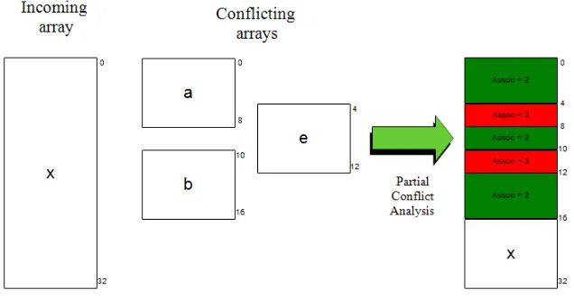
An example of the partial conflict analysis is show in Figure 4.3. We can see that there are three partially conflicting arrays (a,b,e) with the incoming array (x). Composing these conflicts together, the final state of the incoming array is as follows: sets (0-3, 9, 11-16) occupy the second way in the cache. Sets (4-8, 10-12) occupy the third way in the cache. Sets (17-32) occupy the first way in cache. Thus, if the cache is configured for only 2 ways of associativity, this array will partially miss in cache.
Figure 4.3: Partial Conflict Analysis Example
4.5
Handling Varying Strides
When the arrays being analyzed have varying strides, the process of analysis and assigning classifiers changes. It becomes more complex to compensate for two arrays having different strides since one array will be accessing more blocks than the other for the same number of loop iterations.
havecapacity misses. This is a better case than a conflict miss as not all accesses to the array will result in a miss. Also, both of theses arrays are marked to be deleted since only part of each array will be left in the cache at the end of the loop. This is only the case when the conflicting arrays have the same loop depth, i.e., they both belong to the same loop. Arrays with different loop depths are covered in the next sub-section.
However, if the incoming array accesses more blocks than the conflicting array and there are enough ways in the cache, the array is treated as one of the four partial conflict cases, and the appropriate as-sociativities of each chunk of the array are calculated before the analysis proceeds. Both arrays are considered a CONF MISS since they conflict. However, with varying strides there can be some cold/-capacity misses, which will be assigned to the array with the larger stride, i.e., the array which accesses more cache blocks.
This can be generalized as follows:
Context=Context∪ {X} (4.7)
ContextDel=ContextDel∪ {A,X} (4.8)
X←CONF MISS;A←CONF MISS (4.9)
where
A,X = Arrays with varying strides
4.6
Forward Stride Analysis
Recognizing conflicting arrays at a certain loop level as pure conflicts does not necessarily mean they will conflict in outer loops since the strides associated with the arrays for outer loops may vary. Thus, any conflict misses assigned may not necessarily be multiplied by a loop trip count when going from an inner to an outer loop. This situation is difficult to identify and rectify by inspecting the conflict misses in the outer loops given the compostional nature of our analysis. Thus, we perform a forward stride analysis at the loop level when these conflicts have been identified. As the name suggests, the conflicting arrays are analyzed by looking ahead in their stride information and trying to identify potential non-misses. This is done by calculating the number of blocks accessed at each loop level for each array, which can be easily calculated using the stride information per loop level. With this information, it is possible to identify the reduction in the number of conflict misses if any and to then assign a factor for reduction of the misses when the appropriate loop level is reached.
examined. We handle this case by having separate streams for each set of conflicting misses. The reduc-tion factor assigned per stream only modifies the conflict misses predicted for that stream at the time the outer loop level is reached. Thus, controlling conflict misses per stream does not interfere with other streams.
4.7
Handling Varying Loop Depth
Handling conflicting arrays at varying loop depths, i.e., when arrays present in the context information are accessed at either an outer loop nest or an inner loop nest relative to the conflicting array, requires special consideration.
Similar to the previous case, when two arrays are classified to conflict, they do not necessarily experience misses for all accesses to the arrays as misses. A difference in loop depth indicates whether to consider the entire array for conflict analysis or just a single block. The array on the outer loop, i.e., with a lower loop depth, is considered to have conflict misses on all accesses since, for every iteration of the outer loop, the inner loop executes multiple times. And since there is a conflict between an array in the outer loop with an array in the inner loop, the conflicting array in the outer loop will be constantly replaced for each iteration of the outer loop, resulting in a conflict miss for every access of that array. Thus, if any of the conflicting arrays are present in the context and have a lesser loop depth than the incoming array, they need to be removed from the context and have their array classifier updated. Here, the array with the higher loop nesting level is a CONF MISS whereas the array at the lower loop nesting level becomes an ALWAYS MISS since the outer loop array always misses as explained.
This can be defined as:
NX<NA→Context=hContext− {X}i ∪ {A} (4.10) NX>NA→Context=hContext− {A}i ∪ {X} (4.11)
X,A←CONF MISS|ALWAY S MISS (4.12)
where
NX = Loop nesting depth of X
NA = Loop nesting depth of A
4.8
Classifier Modifiers
When an array exceeds cache capacity, all arrays classified as FIRST MISS will change to CAP -MISS, i.e., the capacity misses multiply by the loop length as we move one level from an inner to an outer loop.
4.9
Tracking Cache Capacity and Associativity
With each array addition to the context, the number of ways of the cache and the capacity used by the cache needs to be tracked. This can be done by tracking the maximum number of ways used in both the pure conflict and partial conflict case.
While tracking the number of ways used in the cache, if an array in the context conflicts with the incoming array and if the array in the context has a deeper loop depth, then the number of ways used will be incremented by the number of ways occupied by the new array. However, if both conflicting arrays are inside the same loop, then the number of ways used is only increased by one since we need to keep in mind that the accesses to these arrays are interleaved. Thus, only one block of each array is being accessed per iteration.
Keeping track of used cache capacity is accomplished by aggregating the number of blocks brought into cache per array. This only holds true if the arrays are not conflicting. When arrays conflict, only the blocks that do not conflict needs to be added.
It is also important to keep in mind that the arrays within the loop analysis are considered to be brought into cache block-wise. When calculating the number of ways used or the cache capacity used, the arrays are considered as a whole. Our objective is to analyze the number of ways that will be used by the cache at the end of the loop. Thus, for the intra-loop analysis, each array will be considered block wise for ensuring all arrays can fit within the cache. However, for loop composition, each array has to be considered in its entirety since the entire array should be present in the cache at the end of the loop. The calculation for the number of ways may yield a different result indicating that not all arrays fit within the cache. An example is show in Figure 4.4.
Consider four arrays (a,b,c,d) to fit within a 4-way cache with 4 sets. Each array requires 7 sets and all arrays start at set 0 (a1...a7,b1..b7,c1...c7,d1...d7). Consider one block is accessed per iteration. Thus, during intra-loop analysis, the accesses pattern of the blocks is as follows:a1,b1,c1,d1, ...,a7,b7,c7,d7. With a four way cache, there will not be any conflicts between arrays, which gives the illusion of a FIRST MISS case. However, at the end of the loop, we can see that each array is only partially cached as show in Figure 4.4.
4.10
Special Cases
Figure 4.4: Example of Intra-Loop Analysis
Under certain conditions, the overlap detection algorithms may return false positives. Such a case occurs when the last elements of an array and the first elements of an array share the same block. This is possible since the compiler allocates memory in a contiguous manner and only ensures the data is word aligned, but not block aligned. Such a case should not cause any conflict misses. This can be handled by examining the data returned from the overlap detection and by then continuing analysis ignoring the overlap function.
From the loop depth analysis, we can observe that if an array from the outer loop conflicts with an array of the inner loop, both arrays are marked to be removed from the context. However, for a better analysis model, it would be wiser to keep the inner loop array in context, i.e., only one block of the inner loop array will need to be brought in per outer loop iteration as only one block will conflict between both arrays per outer loop iteration. This can be recorded as an extra conflict miss for the inner loop array.
But this potentially results in an array to be present in the context although it was replaced. This is possible when arrays cross over to many ways. A boundary case exists when an array brought into cache at an inner loop conflicts with more than one array of the outer loop. Thus, this may create a false hits, i.e., the context is checked for an array when it actually is not present. This can be handled by keeping count of the number of ways used and verifying if the all the arrays present in the context (arrays from both the inner and outer loops) can fit into the cache. If the hit is recognized as false hit, conflict misses are assigned instead of hits to the examined array.
Chapter 5
Experimentation Results
This section describes our results in comparison to a cache simulator with respect to execution time and accuracy.
5.1
Test Framework
SMA is compiled using gcc v4.1.2 running on an AMD Opteron machine. The testcases are all in the form of compressed traces as output from ScalaMemTrace. The output from our SMA provides a breakdown of the loops and the number of hits and misses at each loop level.
We also maintain the uncompressed trace file as output by the binary instrumentation tool (PIN). All traces generated were from programs compiled with -O2 optimization to ensure a realistic number of memory accesses performed. The uncompressed trace is fed into a cache simulator to provide output of the same cache statistics as SMA. We use DineroIV [7], a trace-driven uni-processor cache simulator from the University of Wisconsin, as our reference to measure the accuracy and time taken for SMA over a simulation.
5.2
Timing
We assessed a number of test cases for a specific cache configuration and compared the execution times for SMA and DineroIV.
All the experiments utilize a constant cache configuration of 16KB cache size, 64 bytes blocksize and a direct mapped cache.
Figure 5.1: Execution Time for Varying Loop Nest Levels
We observe that SMA has a constant execution time whereas the DineroIV execution time rises exponentially with increasing number of loops.
Figure 5.2 depicts the timing results for increasing matrix sizes in matrix multiplication.
Figure 5.2: Execution Time for Matrix Multiplication
execution time increases exponentially. This is due to the fact that the trace-driven simulator needs to maintain a complete cache state and has to read the traces from an uncompressed file such that I/O becomes a bottle-neck with increasing trace sizes.
Figure 5.3: Execution Time for Matrix Multiplication with Blocking
Figure 5.3 depicts the timing results on a log scale for blocked matrix multiplication with varying block sizes. The timing results here show that the execution is constant for SMA and almost constant for Dinero IV. However, the execution time is much higher for the simulator.
Figure 5.5: Execution Time for NAS Test Cases
Figure 5.4 shows the execution time between SMA and DineroIV on a log scale for test cases from the SPEC CPU 2006 [12] benchmark suite. Figure 5.5 shows the execution time between SMA and DineroIV on a log scale for test cases from the serial version of the NAS [1] benchmark suite v3.3. In most cases tracing with compression of our analysis incurs less overhead on the execution cost then tracing without compression for DineroIV since the latter results in significantly lesser I/O costs. The execution time of our analysis is dependent on the level of compression achieved and the number of arrays present. For EP, our execution is worse than the reference due to insufficient compression achieved resulting in a large number of RSDs present, which requires more time to process.EP, has a conditional statement which generates irregular access patterns and breaks compression.
These timing results have shown that SMA exhibits significantly less execution time compared to a trace driven simulator for a variety of scenarios.
5.3
Accuracy
of nested loops for a given test case.
Figure 5.6: Memory Latency for Nested Loops
The latency is very close to that of DineroIV (under 2%) . It is easier for SMA to handle arrays with constant stride since the complexities of varying strides are not present in these test cases.
We move on to test cases with varying loop depths and array strides and first consider Matrix mul-tiplication. Figure 5.7 shows the memory latency for various matrix multiplication runs for different matrix sizes. We observe that the accuracy remains close to our reference in the most part (within 8%).
However, there are certain spikes in the figure when the data cannot fit in the cache. Thus, more misses are reported with SMA since we do not consider partial arrays to be present within the cache. An other contribution to these extra misses are the array strides exceeding the blocks sizes as mentioned in our special cases (Section:4.10).
Figure 5.8 shows the percent difference in misses between SMA and Dinero IV for the matrix multiply cases. The percent difference in misses in general stays within the 20% range. However, we
Figure 5.8: Percent Miss Difference for Matrix Multiplication
do observe certain small spikes up to around 45%. This can be attributed to small cache sizes, which make analysis harder, when data does not fit within the cache. We also see two big spikes for the 64K cache. These are corner cases where a lot more misses are predicted since we do not track partial data remaining within the cache on conflicts when the arrays exceed cache size.
Figure 5.9 shows the percent difference in miss rate between SMA and Dinero IV. Miss rate here is defined as the difference in the misses divided by the total number of memory references. The miss rate stays within 4% for all the matrix multiply cases. Trends of the percent miss rate mirror the percent difference in misses for the most part. We do not see the spikes here since the total number of references in the two cases are dominant as compared to the misses from SMA or DineroIV.
Figure 5.9: Percent Miss Rate Difference for Matrix Multiplication
with the case when an array stride exceeds the block size as discussed in Section 4.10, which makes it harder to analyze such cases. However, this can be an indicator that no spatial locality is present in the application.
Figure 5.11 shows the percent difference in misses between SMA and Dinero IV for matrix multiply with blocking cases. The percent differences in misses stays within the 40% range in many cases. There are a few spikes which lie between 60-80%. Theses are usually due to the smaller cache sizes that retain partial data not considered by our analysis. There is one dominant spike, which again due to a small cache size, where we report more conflict misses than there actually may be since the arrays analyzed exceed cache capacity so that conflict analysis is not performed.
Figure 5.12 shows the percent difference in miss rate between SMA and Dinero IV for matrix multiply with blocking cases. The percent miss rate is similar to the percent difference in misses for the most part. We do see similar spikes as before. However, the miss rate stays within 8% for all the test cases.
Figure 5.13 shows the memory latency results for test cases from the SPEC CPU 2006 [12] bench-mark suite. Most test cases are within a 6% difference in latency. There are a few spikes at the beginning, again attributed to the small cache size and data accessed exceeding the cache size.
Figure 5.14 shows the percent difference in misses between SMA and Dinero IV for the SPEC benchmark test cases. We observe a slightly different trend in this case. Most of the differences are within a 40% range. There are few spikes above this region for lower cache sizes for the same reason as seen in the figure 5.13.
Figure 5.10: Memory Latency for Matrix Multiplication with Blocking
spikes from the percent difference in misses is not seen here since the number of memory references far exceeds the difference in misses. We stay within a 3% difference except for two outliers for small cache sizes for the same reasons as the previous figure.
Figure 5.16 shows the memory latency results for the serial version of test cases from the NAS [1] benchmark suite v3.3. The accuracy of the cases varies with different cache configurations. We observe 3 of the 5 cases do very well and stay within a 1-2% difference in latency.FTspikes in low cache sizes. MGperforms consistently worse than the others due to varying strides and partial data overlap that is not accounted for in our analysis. However, we still stay within a 9% difference from our reference.
Figure 5.17 shows the percent difference in misses between SMA and Dinero IV for the NAS bench-mark test cases. Here, most of the test cases differs by less than 40%. There are a few outliers for small cache sizes. There is one spike forMG, which is due to partial data overlap not accounted for in our analysis.
Figure 5.18 shows the percent difference in miss rate between SMA and Dinero IV for the NAS benchmark test cases. The figure again follows the trends of the percent difference in memory latency. Most case lie within a 2% difference and overall a 4% difference since the number of memory references far exceeds the number of misses in most cases by 1-2 orders of magnitude.
5.4
Case Study
Figure 5.11: Percent Miss Difference for Matrix Multiplication with Blocking
64B blocksize and is 2-way associative. We expose the compressed trace for the same execution to our analysis and compare the results.
For timing purposes, we recorded the uncompressed trace for the first three cases and compared the execution time on a logarithmic scale between SMA and DineroIV as shown in Figure 5.19. Our SMA has a near constant execution time due to perfect compression properties of matrix multiply. However, DineroIV follows an exponential trend and does not scale well. The figure only shows the first three points for DineroIV since the simulation time had exceeded 30 minutes, which made it unfeasible to continue time larger test cases.
In Figure 5.20, we represent the three metrics we have introduced for accuracy, i.e., the percent difference in misses, the percent difference in miss rate and the percent difference in memory latency between SMA and the hardware counters. Our results stay well within a 5% difference for all cases which indicates that our method can scale easily to large problems. There is a single spike in the graph which is due to the way the data strides in the memory. More partial data is retained in this case in the outer loops resulting in fewer misses, which is not accounted for by our analysis.
Figure 5.12: Percent Miss Rate Difference Matrix Multiplication with Blocking
Figure 5.14: Percent Miss Difference for SPEC Benchmark Suite
Figure 5.16: Memory Latency for NAS Benchmark Suite
Figure 5.18: Percent Miss Rate Difference for NAS Benchmark Suite
Chapter 6
Related Work
Previous work on cache analysis [18] utilizes compressed traces have been used. But their approach does not consider the problem of identifying data structures causing cache misses. Janapsatya et al. [15] talk about compressing program traces and perform a partial decompression for cache simulation.
The idea of reuse distanceto predict reuse patterns of the whole program [9] and to use the reuse distances to estimate capacity miss rates of a fully associative cache [24] have been explored. StatCache [2] is a sampling-based data-locality technique analysis for fully associative caches. Reuse distance has also been used to provide cache hints [3] to specify at which cache level the data is likely to be found.
Dinero IV [7], is one of many toold to support exact cache simulation for an uni-processor archi-tecture given a cache configuration. The also exists work on trace-driven multi-processor simulation [14, 13, 6]. Some compression techniques which have reduced I/O when passed to a trace-driven simu-lator [17, 16]. However, the processing of theses traces before simulation does not provide a significant speedup in execution time.
Chapter 7
Future Work
Our attempt at a compositional approach towards cache analysis is only the beginning. The first im-provement would be to improve the accuracy in the case of handling strides that exceed the block size (Section 4.10). Another improvement can be to provide suggestions to users by identifying and reporting highly conflicting data structures.
SMA is currently only targeted for uni-processor systems. This can be generalized to instantiating the tool per thread basis. Thus, one may analyze cache performance of multi-threaded programs and eventually make it possible to extrapolate the memory behavior of multi-threaded applications to larger number of threads.
Chapter 8
Conclusion
Uncompressed trace-driven simulation requires excessively large trace files and maintains complete cache states which, increases computation time and may not scale as trace sizes increase. The simula-tion output may be hard to analyze to pin-point performance bottle-necks of an applicasimula-tion. We utilize ScalaMemTrace [4] to obtain trace files from applications running under PIN, a binary instrumenta-tion tool. Such traces contain the memory addresses referenced, a unique signature associated with the memory access and the type of access (load/store). We then perform on-the-fly compression and produce compressed trace file in the form RSD/PRSDs.
We have developed ScalaMemAnalyis, a novel approach towards compostional cache analysis from compressed traces that uses an extended version of the reuse distance theory. We use a context-based reuse distance analysis to maintain information of arrays (i.e., a strided RSD) that can fit within a cache, given the cache configuration, i.e., the cache size, block size and associativity. The key criteria to ensure data structures can fit within the cache and remain within the cache are cache capacity and associativity. We discuss conflict cases and we develop a method to handle varying loop nesting depths and strides within the analysis and special cases which need to be considered.
REFERENCES
[1] David H Bailey, Eric Barszcz, John T Barton, David S Browning, Russell L Carter, Leonardo Dagum, Rod A Fatoohi, Paul O Frederickson, Thomas A Lasinski, Rob S Schreiber, et al. The NAS parallel benchmarks. International Journal of High Performance Computing Applications, 5(3):63–73, 1991.
[2] Erik Berg and Erik Hagersten. StatCache: a probabilistic approach to efficient and accurate data locality analysis. In Performance Analysis of Systems and Software, 2004 IEEE International Symposium on-ISPASS, pages 20–27. IEEE, 2004.
[3] Kristof Beyls and Erik H DHollander. Reuse distance-based cache hint selection. InEuro-Par 2002 Parallel Processing, pages 265–275. Springer, 2002.
[4] Sandeep Budanur, Frank Mueller, and Todd Gamblin. Memory trace compression and replay for SPMD systems using Extended PRSDs. The Computer Journal, 55(2):206–217, 2012.
[5] Pat Conway, Nathan Kalyanasundharam, Gregg Donley, Kevin Lepak, and Bill Hughes. Cache hierarchy and memory subsystem of the AMD Opteron processor. IEEE micro, 30(2):16–29, 2010.
[6] Luiza MN Coutinho, Jos´e Leandro D Mendes, and Carlos APS Martins. Mscsim-multilevel and split cache simulator. InFrontiers in Education Conference, 36th Annual, pages 7–12. IEEE, 2006.
[7] Trace-Driven Uniprocessor Cache Dinero IV. Simulator. URL: http://www.cs.wisc.edu/˜markhill/DineroIV, 2012.
[8] Chen Ding and Yutao Zhong. Reuse distance analysis. University of Rochester, Rochester, NY, 2001.
[10] Somnath Ghosh, Margaret Martonosi, and Sharad Malik. Cache miss equations: An analytical representation of cache misses. InProceedings of the 11th international conference on Supercom-puting, pages 317–324. ACM, 1997.
[11] Paul Havlak and Ken Kennedy. An implementation of interprocedural bounded regular section analysis. Parallel and Distributed Systems, IEEE Transactions on, 2(3):350–360, 1991.
[12] John L. Henning. SPEC CPU2006 Benchmark Descriptions. SIGARCH Comput. Archit. News, 34(4):1–17, September 2006.
[13] Ravi Iyer. On modeling and analyzing cache hierarchies using CASPER. In Modeling, Anal-ysis and Simulation of Computer Telecommunications Systems, 2003. MASCOTS 2003. 11th
IEEE/ACM International Symposium on, pages 182–187. IEEE, 2003.
[14] Aamer Jaleel, Robert S Cohn, Chi-Keung Luk, and Bruce Jacob. CMP $im: A Pin-based on-the-fly multi-core cache simulator. InProceedings of the Fourth Annual Workshop on Modeling, Benchmarking and Simulation MoBS, co-located with ISCA, pages 28–36, 2008.
[15] Andhi Janapsatya, Aleksandar Ignjatovic, Sri Parameswaran, and Joerg Henkel. Instruction trace compression for rapid instruction cache simulation. InProceedings of the conference on Design, automation and test in Europe, pages 803–808. EDA Consortium, 2007.
[16] E.E. Johnson, Jiheng Ha, and M. Baqar Zaidi. Lossless trace compression. Computers, IEEE Transactions on, 50(2):158–173, Feb 2001.
[17] Eric E Johnson and Jiheng Ha. Lossless address trace compression for reducing file size and access time. InInternational Phoenix Conference on Computers and Communications, IEEE Press, Los Alamitos, CA, USA, pages 213–219. Citeseer, 1994.
[19] Chi-Keung Luk, Robert Cohn, Robert Muth, Harish Patil, Artur Klauser, Geoff Lowney, Steven Wallace, Vijay Janapa Reddi, and Kim Hazelwood. Pin: building customized program analysis tools with dynamic instrumentation. ACM Sigplan Notices, 40(6):190–200, 2005.
[20] Jaydeep Marathe, Frank Mueller, Tushar Mohan, Sally A Mckee, Bronis R De Supinski, and Andy Yoo. METRIC: Memory tracing via dynamic binary rewriting to identify cache inefficiencies. ACM Transactions on Programming Languages and Systems (TOPLAS), 29(2):12, 2007.
[21] Philip J Mucci, Shirley Browne, Christine Deane, and George Ho. PAPI: A portable interface to hardware performance counters. InProceedings of the Department of Defense HPCMP Users Group Conference, pages 7–10, 1999.
[22] Frank Mueller. Timing analysis for instruction caches.Real-Time Systems, 18(2-3):217–247, 2000.
[23] Wikipedia. Cache Miss — Wikipedia, The Free Encyclopedia.http://en.wikipedia.org/wiki/CPU -cache#Cache miss.
Appendix A
Code Samples
A.1
Sample RSD/PRSD
A.1.1 Loop Frame
The following frame indicates the beginning of a loop. The loopsize indicates number of frames follow-ing this frame that are present in the loop. The loopcount indicates the number of iterations of the loop. The sign field in this case is a dummy sign since it is a dummy frame to indicate the beginning of the loop.
attr:3 loopsize:6 loopcount:4 sign:0xc0ffeefeedc0ffee
gap: 0
start_value: (nil)
length: 4
stride: (nil)
tid_start_value: (nil)
tid_length: 1
tid_stride: (nil)
tid_bit_pattern: 0x1
tid_addr_stride: (nil)
node_id_start_value: (nil)
node_id_length: 1
node_id_stride: (nil)
node_id_bit_pattern: 0x1
Sign_len = 1
Sign:0xc0ffeefeedc0ffee
ref_id = 0xc0ffeefeedc0ffee
A.1.2 Standard Frame
This frame is similar to the loop frame. The first sign field contains an XOR of the different signatures obtained from a stackwalk. All the original signatures are indicated in the second sign field.
The type field indicates if the frame represents a load or store instruction
• Type 0x6c = ascii ”l” = Load frame
• Type 0x73 = ascii ”s” = Store frame
attr:5 loopsize:0 loopcount:1 sign:0x400437
gap: 0
start_value: 0x7fffe5cc7c7c
length: 1
stride: 0x4
tid_start_value: (nil)
tid_length: 1
tid_stride: (nil)
tid_bit_pattern: 0x1
tid_addr_stride: (nil)
node_id_start_value: (nil)
node_id_length: 1
node_id_stride: (nil)
node_id_bit_pattern: 0x1
Sign_len = 3
Sign:0x4004e1 0x4004bb 0x40046d
ref_id = 0x400437