Extension of low-thrust propulsion to the autonomous coplanar circular restricted four body problem with application to future Trojan Asteroid missions

to the autonomous coplanar circular restricted four body problem with

application to future Trojan Asteroid missions. In: 61st International

Astronautical Congress, IAC 2010, 2010-09-27 - 2010-10-01. ,

This version is available at

https://strathprints.strath.ac.uk/27453/

Strathprints is designed to allow users to access the research output of the University of Strathclyde. Unless otherwise explicitly stated on the manuscript, Copyright © and Moral Rights for the papers on this site are retained by the individual authors and/or other copyright owners. Please check the manuscript for details of any other licences that may have been applied. You may not engage in further distribution of the material for any profitmaking activities or any commercial gain. You may freely distribute both the url (https://strathprints.strath.ac.uk/) and the content of this paper for research or private study, educational, or not-for-profit purposes without prior permission or charge.

Any correspondence concerning this service should be sent to the Strathprints administrator: [email protected]

The Strathprints institutional repository (https://strathprints.strath.ac.uk) is a digital archive of University of Strathclyde research outputs. It has been developed to disseminate open access research outputs, expose data about those outputs, and enable the

Ceccaroni, M. and Biggs, J.D. (2010) Extension of low-thrust propulsion to the autonomous coplanar

circular restricted four bidy problem with application to future Trojan Asteroid missions. In: 61st

International Astronautical Congress, IAC 2010, 27 Sept -1 Oct 2010, Prague, Czech Republic.

http://strathprints.strath.ac.uk/

27453

/

Strathprints is designed to allow users to access the research output of the University of

Strathclyde. Copyright © and Moral Rights for the papers on this site are retained by the

individual authors and/or other copyright owners. You may not engage in further

distribution of the material for any profitmaking activities or any commercial gain. You

may freely distribute both the url (http://strathprints.strath.ac.uk) and the content of this

paper for research or study, educational, or not-for-profit purposes without prior

permission or charge. You may freely distribute the url (http://strathprints.strath.ac.uk)

of the Strathprints website.

EXTENSION OF LOW-THRUST PROPULSION TO THE AUTONOMOUS COPLANAR CIRCULAR RESTRICTED FOUR BODY PROBLEM WITH APPLICATION TO FUTURE

TROJAN ASTEROID MISSIONS

Marta Ceccaroni

Advanced Concepts Space Laboratory, Glasgow, UK [email protected]

James Biggs

Advanced Concepts Space Laboratory, Glasgow, UK [email protected]

An Autonomous Coplanar Circular Restricted Four Body Problem (CRFBP) is considered, where the massless body is a low-thrust spacecraft. “Natural” and “artificial” (i.e. created with the use of continuous low-thrust propulsion) equilibrium solutions are identified, that have the potential to be exploited in future science missions. Results show that, with zero thrust, there are unstable equilibrium points close to the third primary. However, artificial equilibrium points, displaced from the natural ones, can be generated with the use of constant low-thrust. Furthermore, these points are proved to be stable in certain regions about the third primary mass. This is particularly advantageous since it means that it would be possible to continuously maintain a spacecraft about these strategic observation points, close to the smaller primary, without the need for state feedback control. The Sun-Jupiter-Trojan Asteroid-Spacecraft system is considered, as a particular case of the Autonomous Coplanar CRFBP. Curves of artificial equilibrium points are then identified. Furthermore, the stability analysis of these points reveals the region where they are stable. In this region four bounded orbits close to the Asteroid are proved to exist, that can be reached and maintained with a constant low-thrust lower than10µN.

Key words:Four Body Problems·Low-thrust Propulsion·L4·Trojan Asteroid

I. INTRODUCTION

The use of continuous low-thrust propulsion in four body systems could enable a range of potential appli-cations for several fields such as space physics, human exploration, planetary science, asteroid observation and many more.

The present studies on the dynamics of four body problem fall into two general categories:

• where the CRFBP is analyzed as a perturbed Three Body Problem (Hill’s approximation). In this case the fourth body is set to be at a large distance from the other assumed three bodies such that it can be considered a perturbation.

Two examples of this case can be found in Scheeres [1], and the bicircular model considered by Cronin et al.[2], where both models are used to approximate the dynamics of the Sun-Earth-Moon-Spacecraft system;

• where two or three of the primary masses are set to be equal and the planets are in a particular

configura-tion such as the Symmetric, Collinear CRFBP (see [3] or [4]). Generally speaking these systems are motivated by mathematical interest rather than a particular application.

On the other hand, the use of continuous low-thrust propulsion, has so far been confined to two and three-body systems. Space mission design for low thrust spacecraft has been extensively investigated from the late 1990’s. So far the two major types of low-thrust propulsion, which have been studied in this context, are solar sails and solar electric propulsion (SEP), the latter considered in this paper.

Research on this topic are, at present, mainly focussed on finding artificial equilibria as in [5], [6] or [7], on generating periodic halo orbits (see, for example, [8], [9] or [10]), or on the systematic cataloguing of non-Keplerian orbits as in [11].

In this paper the interaction between these two relatively new topics is considered and explored both for mathematical interest as well as to identify possible applications for mission design.

To this end an Autonomous Coplanar CRFBP is

zed, with the objective of identifying completely new orbits for future mission applications.

A low-thrust spacecraft is assumed, on the basis of the technical capability of the QinetiQ thrusters [12], which can generate a thrust of approximately250mN. Moreover we assume a capability of 300mN maxi-mum thrust to account for feasible future advances in low-thrust propulsion systems.

Results show that, with zero thrust, there are unstable equilibrium points close to the third primary. However, artificial equilibrium points, displaced from the natural ones, can be generated with the use of constant low-thrust. Furthermore, these points are proved to be stable in certain regions about the smaller primary. This is particularly advantageous since it means that it would be possible to maintain a spacecraft around strategic observation points about the third primary continuously without the need for state feedback control.

Finally, the particular case of the Sun-Jupiter-Asteroid-Spacecraft Autonomous Coplanar CRFBP is analyzed. In this case the third primary mass is taken to be small to reflect estimates of asteroid masses predicted to be trapped at the triangular Lagrangian points of the Sun-Jupiter-Spacecraft system. Curves of artificial equilibrium points are then identified. The stability analysis of these points reveal the region where they are stable.

This investigation could potentially be useful for designing missions to the Jupiter Trojans. This set of asteroids, captured around theL4andL5points of the Sun-Jupiter-Spacecraft system, has been recognized as present target for space science missions; furthermore, understanding them may lead to clues to the origin and dynamical evolution of Jupiter itself [13]. Currently, the Trojan Asteroids are completely unexplored and largely unknown and any visit by a spacecraft will revolutionize our current understanding of these bodies [14]. Moreover, this paper highlights the possibility to maintain strategic observation points close to a Jovian Trojan with reduced requirements on fuel and without the need for a state feedback control.

II. THE AUTONOMOUS COPLANAR CRFBP

The Autonomous Coplanar Circular Restricted Four Body Problem (CRFBP) is the problem of describing the dynamics of the motion of a “zero mass” body

PS subject to the gravitational field generated by an

assigned three body system (P1, P2 and P3) on a two dimensional space. In this paper we analyze this problem with the additional assumption that the third

PrimaryP3has to be small enough such that it does not effect the motion of the other two massive bodies (and, for this reason, it will be identified hereafter with the generic name of “Asteroid”).

The position of the Asteroid is set to correspond to one of the triangular Lagrangian points of the

P1−P2−Spacecraf tRestricted Three Body System, which means that the Primaries form an equilateral triangle. It is well known, in fact, that these points are stable for values of the mass parameterµsmaller than Routh’s critical mass −9±

√

69

18 in non-dimensional units [15].

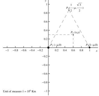
Moreover the orbits of the three Primaries are taken to be circular, revolving around the barycenter of P1 and P2 with constant angular velocity ω such that, choosing a frame of reference Ox,y, centered in the

center of rotation and revolving with the same angular velocityωof the bodies, the three masses are fixed. The units of distance and mass are then scaled with the dis-tance betweenP1andP2and the sum of their masses respectively, while the gravitational constantGand the rotational velocityωare set to be one.

In this non dimensional units letµ,1−µandǫbe the scaled mass ofP2,P1andP3respectively:

µ= m2

m1+m2 1−µ= m1

m1+m2

ǫ= m3

m1+m2

As the planets are fixed and the origin of the system of reference is set in the barycenter of the major pri-maries, we can, without loss of generality, take the po-sition ofP1andP2to be(−µ,0)and(1−µ,0) respec-tively, which implies that the position of the Asteroid (see [16]) must be(Lx, Ly) = (1₂−µ,

√

3

2 )as in Fig.1.

P3H

1 2

-Μ, 3 2

L

P1H-Μ,0L P2H1-Μ,0L

PSHx,yL

Unit of measure 1=106_Km

y

x 0.2 0.4 0.6 0.8

-0.2

-0.4

-0.6

-0.8 1

-1

0.2 0.4 0.6 0.8

-0.2

-0.4

-0.6

-0.8 1

-1

The dynamics of the massless spacecraft (whose po-sition is expressed in non-dimensional cartesian coor-dinatesx, y) is described by the system:

_¨

x= 2 ˙y−∂Ω

∂x

¨

y=−2 ˙x₋∂_∂yΩ (1)

were theaugmentedoreffectivepotential is:

Ω =−x

2_+y2

2 − (1−µ)

r1 −

µ r2 −

ǫ r3

the distance of the spacecraft from each of the three primaries is:

r1=p(x+µ)2+y2

r2= p

(x+µ−1)2_+y2

r3=p(x−Lx)2+ (y−Ly)2

∂Ω

∂x ( ∂Ω

∂y), denotes the partial derivative of Ω with

respect tox(y), while the “dot” denotes the differenti-ation with respect to time.

In order to find the equilibrium points of the system, the velocitiesx,˙ y˙and the accelerations¨x,y¨are set to be zero in (1) obtaining:

∂Ω

∂x = 0 ∂Ω

∂y = 0

(2) Or equivalently                   

x− (1−µ)(x+µ)

√

(x+µ)2 +y2 3−

µ(x−(1−µ))

√

(x−(1−µ))2 +y2 3

− ǫ(x−Lx) q

(x−Lx)2 +(y−Ly)23

= 0

y− (1−µ)y √

(x+µ)2 +y2 3−

µy √

(x−(1−µ))2 +y2 3

−q ǫ(y−Ly) (x−Lx)2 +(y−Ly)23

= 0

(3)

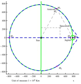
The green, continuous and the blue, dashed lines in Figure 2 represents the first and the second equation of system (3) respectively; the two lines intersect only six times forming the equilibrium points of the system as it would become clear zooming in as in Figure 3.

Asteroid

Sun Jupiter

M1 M2 M3

M4 M5

M6

Spacecraft

200 400 600 800

-200 0

-400 -600 -800 200 400 600 800 -200 -400 -600 0 -800

Unit of measure 1=106_{Km x}

y

Figure 2: Equilibrium Points; the six intersections of the lines are the solutions of system (3): the equi-librium points of the system.

Asteroid

M4

M5

388.414 388.418 388.422 388.426 388.429 388.433 674.042 674.045 674.049 674.053 674.057 674.061 674.065

Unit of measure 1=106

Km x

y

Figure 3: Equilibrium Points; zooming on the Asteroid and the two equilibrium points close to it.

The qualitative dynamics close to the asteroid do not change for different massesǫ_∈ (0, µ)of the Asteroid in that there are always two equilibrium points config-ured approximately at the same angle relative to the as-teroid. However, quantitatively, as the mass increases the equilibrium points are displaced further from the asteroid, as shown in Figure 4. Thus, we would con-clude that the only assumption on the mass of the As-teroid is that it has to be small enough such that it does not affect the motion of the other two Primaries.

3 2 1 3 2 1 L L L L 1

1 ® m3=1014_Kg

2 ® m3=1015_Kg

3 ® m3=1016_Kg

Asteroid

388.414 388.418 388.422 388.426 388.429 388.433 674.042 674.045 674.049 674.053 674.057 674.061 674.065

Unit of measure 1=106_{Km x}

y

Figure 4: Equilibrium Points;∀ǫ_∈(0, µ)the two lines intersects twice in the region close to the Asteroid.

Hereafter, for simplicity of notation, (xe, ye) will

indicate a generic equilibrium solution of system (3).

III. STABILITY ANALYSIS

For the stability analysis a translation of the coordi-nates to the generic equilibrium point(xe, ye)is

per-formed.

x′=x−xe

y′ _=y−y

e (4)

For simplicity of notation the indices abovex′andy′

are ignored.

The linearized motion close to the point(xe, ye)is:

       ˙

x=vx

˙

y=vy

˙

vx= 2vy+αx+χy

˙

vy=−2vx+χx+βy

(5)

with

α= 1 +(1−µ)

h

2(xe+µ)2−ye2i

q

(xe+µ)2 +y2

e

5 +

µh2(xe+µ−1)2−ye2i

q

(xe+µ−1)2 +y2

e

5

+ǫ

h

2(xe−Lx)2−(ye−Ly)2i q

(xe−Lx)2 +(ye−Ly)25

β= 1 +(1−µ)

h

−(xe+µ)2 +2ye2i

q

(xe+µ)2 +y2

e

5 +

µh−(xe+µ−1)2 +2ye2i

q

(xe+µ−1)2 +y2

e

5

+ǫ

h

−(xe−Lx)2 +2(ye−Ly)2i q

(xe−Lx)2 +(ye−Ly)25

χ= 3

(

(1−µ)[(xe+µ)ye] q

(xe+µ)2 +y2

e

5 +

µ[(xe+µ−1)ye]

√

(xe+µ−1)2 +ye+25

+qǫ[(xe−Lx)(ye−Ly)] (xe−Lx)2 +(ye−Ly)25

)

Therefore the four eigenvalues of the system are:

Ψ1,2=± r

−(4−α−β)+√(4−α−β)2−4αβ+4χ2 2

Ψ3,4=± r

−(4−α−β)−√(4−α−β)2−4αβ+4χ2 2

(6)

It can be shown that, fixing a specific massǫ_∈(0, µ)

for the Asteroid, and evaluating the eigenvalues corre-sponding to both the equilibrium points, only one of them will have positive Real part, which implies that the natural equilibrium points are bothsaddle×center

points, i.e. linearly unstable, and therefore nonlinearly unstable.

Evaluating the eigenvalues for the Sun-Jupiter-Trojan Asteroid-Spacecraft system, where the mass of the Asteroid is set to be1015_{Kg(reasonable, since the} total mass of all the Trojan Asteroids is equal to0.0001

times the mass of the Earth∼5.9736×1020_{Kg). Then,} as expected, both the equilibrium pointsM4 andM5 are unstable.

In particular, in non dimensional units, evaluating them inM4= (M4x, M4y) = (0.499044; 0.866021)yields:

Ψ1,2=±2.07049

Ψ3,4=±2.50695i

While forM5 = (M5x, M5y) = (0.499049; 0.86603)

we find:

Ψ1,2=±2.07047

Ψ3,4=±2.50693i

IV. THE LOW-THRUST AUTONOMOUS COPLANAR CRFBP

The idea of this paper is to investigate the dynamics of a low-thrust spacecraft in the Autonomous Coplanar

CRFBP. Using the thrust propulsion our spacecraft can create artificial equilibrium points suitable for Asteroid observation missions. In addition a subset of these novel equilibrium points are proved to be stable such that the motion will remain bounded in a small region about them, with relatively low fuel requirements and without the need for a state feedback control.

Given a maximum thrusting capabilityF expressed inmN, which can be developed by the spacecraft, and an approximate weight for the spacecraft Ws,

eval-uated in Tons, the maximal acceleration in the non-dimensional units is given by:

anondim =WsF mN

T =F×

10−6

Ws · m s2 = F×10−6

Ws · Kg m2 m

3

Kg·s2 = F×_Ws10−6 d

2

P₁/P₂

(m1+m2)

1

G

(7)

wheredP1/P2means the distance in meters between the

two major Primaries.

Indicating the acceleration withanˆ=axx¯+ayy¯where

a=qa2

x+a2yis the magnitude andnˆis the direction

of the acceleration itself,awill therefore be contained in(0;anondim).

As mentioned in previous sections, an optimistic but realistic, “near term”, reachable maximal thrusting powerFis taken to be300mN.

In order to estimate the range of possible acceleration on the spacecraft we fix it’s mass to be1T.

For the Sun-Jupiter-Trojan Asteroid-Spacecraft system the non-dimensional value of the maximum accelera-tionanondimwill therefore be1.36765.

Moreover the acceleration has to be constant in the direction of the perturbation, namely

∂

∂x(anˆ) = ∂

∂y(anˆ) = 0 (8)

Adding low-thrust to system (1) it becomes:

¨

x= 2 ˙y₋∂_∂xΩ+ax

¨

y=−2 ˙x−∂Ω

∂y +ay

(9)

with

Ω =−x2+2y2 − (1−µ)

r1 −

µ r2 −

ǫ r3

a=qa2

x+a2y ≤anondim

r1=

p

(x+µ)2_+y2

r2=

p

(x+µ₋1)2_+y2

r3=

p

(x₋Lx)2+ (y−Ly)2

Again, to find the equilibrium points, the velocities

˙

ax=∂_∂xΩ

ay= ∂_∂yΩ (10)

That can also be seen as:

_a=

|∇Ω|

ˆ

n=−∇Ω

|∇Ω|

(11)

System (11) states that, in order to get a new equilibrium point, the acceleration on the spacecraft due to the thrusters has to be equal in magnitude (first equation) but opposite in direction (second equation) to the acceleration on the spacecraft due to the gravitational field at that point.

V. STABILITY ANALYSIS OF THE LINEARIZED SYSTEM

Notice that, with a constant thrust, system (9), once linearized, is equal to the linear system in (5) and therefore the linear stability of the equilibrium points resulting from system (11) will be given by the analysis of the eigenvalues in (6).

By the Lyapunov Stability theorem (see for example [17]), in order to obtain a linearly bounded motion, the eigenvalues must have Real part less than or equal to zero. In our case, recall (6), we cannot have a non zero Real part, as it would imply thatRe(Ψ1)> 0or

Re(Ψ2) = Re(−Ψ1) = −Re(Ψ1) > 0 and/or the same forΨ3,Ψ4, thus leading to asaddle×saddle or a saddle × center unstable equilibrium point respectively.

Therefore, in this case, it is only possible to have linearly bounded motion where Re(Ψk) = 0,

k= 1,2,3,4

Thus, recalling (6), the conditions for the four eigenvalues to be purely Imaginary are:

(4−α−β)2

−4αβ+ 4χ2

≥0

−(4−α−β) +p

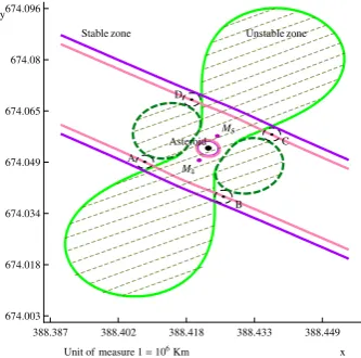
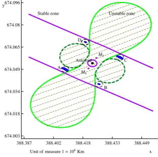
(4−α−β)2_{−4αβ+ 4χ}2_≤0 (12)

System (12) is satisfied by the “stable zone” of Figure 5.

In particular the first inequality of the system is verified by the points outside the dark-green, dashed line, while the second by those outside the green, continuous line. The intersection of these two zones, namely the external part of the “four leaf clover” zone, is then the area in which the linearized motion is stable. Notice that, as shown before, the equilibrium pointsM4 and

M5are linearly unstable.

Asteroid

M4 M5

Unstable zone Stable zone

388.387 388.402 388.418 388.433 388.449 674.003

674.018 674.034 674.049 674.065 674.08 674.096

Unit of measure 1=106_{Km x}

y

Figure 5: Linearly stable-unstable zones; system (12) is satisfied by the points outside the “four leaf clover”, the linearly stable zone.

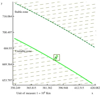
Of course there exist an external limit of the linearly stable zone as represented in Figure 6. In particular the first inequality of the system is verified by the points between the dark-green, dashed lines, while the second by those between the green, continuous lines. The in-tersection of these two zones is then the actual area in which the linearized motion is stable.

Unstable zone Stable zone

350.249 365.815 381.382 396.948 412.515 428.082 653.797

669.364 684.93 700.497 716.064

Unit of measure 1=106_{Km x}

y

Figure 6: The external stability boundary of the linearly stable zone;(for displaying purpose the zone inside the square is magnified by∼50times).

In the Sun-Jupiter-Trojan Asteroid-Spacecraft sys-tem, the maximal possible thrust to remain within the stability boundary will approximately be of magnitude

0.4826mN.

Anyway, in this paper, the actual thrust used is lower than10µN, that will enable to create artificial equilib-rium points in the area between the two dark, purple lines in Figure 7.

Four artificial equilibrium points A, B, C, Dare chosen in the linearly stable zone, at a distance from the

unstable zone equal or higher than 2000km (see Figure 7), since we want to remain as close as possible to the Asteroid but far enough from the unstable zone, such that even with injection errors the spacecraft will remain in the stable zone (see Fig 7).

For the Sun-Jupiter-Trojan Asteroid-Spacecraft sys-tem the four points are at a distance of approximately

15000kmfrom the Asteroid.

Asteroid M4

M5

Unstable zone Stable zone

A

B C D

388.387 388.402 388.418 388.433 388.449 674.003

674.018 674.034 674.049 674.065 674.08 674.096

Unit of measure 1=106_{Km x}

y

Figure 7: Adding the low-thrust; using a thrust lower than10µN, four equilibriaA, B, C, D are cre-ated in the stable zone, reachable with a thrust

∼0.0089mN.

To evaluate the thrust required to create an artificial equilibrium point, for example inA = (Ax;Ay), the

computation of the gravitational field in this point is needed.

In the Sun-Jupiter-Trojan Asteroid-Spacecraft system, in non-dimensional units, it is:

ax=−Ax+√(1−µ)(Ax+µ)

(Ax+µ)2_+A2

y

3 +

µ(Ax+µ−1)

√

(Ax+µ−1)2_+A2

y

3

+√ ǫ(Ax−Lx)

(Ax−Lx)2_+(Ay−Ly)23 =−0.0000195028

ay=−Ay+√ (1−µ)Ay

(Ax+µ)2_+A2

y

3 +

µAy √

(Ax+µ−1)2_+A2

y

3

+√ ǫ(Ay−Ly)

(Ax−Lx)2_+(Ay−Ly)23 =−0.000035642

(13) Such that the magnitude of required thrust is:

a=qa2

x+a2y = 0.0000406289(∼0.0089mN)

(14) This thrust is represented by the pink line in Figure 7 and, as we can clearly see, it is approximately the same thrust required to create the other three equilibrium

pointsB,CandD.

We will analyze in detail the motion forA, since all the four points have similar behaviors as we will show graphically later on.

VI. INTEGRATING THE LINEARIZED MOTION

CallingAthe Jacobian matrix corresponding to system (5), namely:

A=



  

0 0 1 0

0 0 0 1

α χ 0 2

χ β −2 0



  

(15)

The eigenvectors of the system are four vectors fj ∈

C4_{, j= 1, ...,4such that}

Afj= Ψjfj, j= 1, ...,6 (16)

Recalling that linearizing the system (9) yields the linear system (5), whose eigenvalues are those in (6), we take an equilibrium point within the linearly stable zone (i.e. with purely imaginary eigenvalues), and thus rearrange the eigenvalues in the form:

Ψ1=λi

Ψ2=−λi

Ψ3=νi

Ψ4=−νi

(17)

where

λ=

q

(4−α−β)−√(4−α−β)2_−4αβ+4χ2

2

ν=

q

(4−α−β)+√(4−α−β)2_−4αβ+4χ2

2

(18)

λ,µ_∈R_.

Being the eigenvalues two couples of complex con-jugated values, the eigenvectors must be concon-jugated too, namelyf2 =f1∗andf4 = f3∗, and therefore we

need just to findf1andf3.

With a few algebraic manipulations it is possible to calculate their explicit expressions:

f1= [1,−_β+χ_λ2,0,−

2λ2

β+λ2]T +i[0,_β+2λ_λ2, λ,−

χλ β+λ2]T

f3= [1,−χ(α+ν

2

)

χ2_+4ν2,0,−

2ν2(α+ν2)

χ2_+4ν2 ]T +i[0,2ν_χ2(α₊₄+_νν22), ν,−

χν(α+ν2₎

χ2_+4ν2 ]T

(19)

M=      

1 0 1 0

−β+χλ2 β+2λλ2 −

χ(α+ν2 ) χ2 +4ν2

2ν(α+ν2 ) χ2 +4ν2

0 λ 0 ν

− 2λ2 β+λ2 −

χλ β+λ2 −

2ν2 (α+ν2 ) χ2 +4ν2 −

χν(α+ν2 ) χ2 +4ν2 )

      (20)

Applying the transformation of coordinatesM−1 _on

X= [x, y, vx, vy]T, yields the new coordinates

ג_{= [ξ1, ξ2, ψ1, ψ2]}T_{, namely:}

ג_=M−1_{X (21)}

The transformationM is performed on the system (5) to find it’s expression in the new coordinates:

˙

ג_=M−1_˙

X=M−1AX=M−1A Mג (22)

that can be rewritten as:

˙

ג_=A′ג _{with A}′_=M−1_{A M (23)}

WhereA′_is:

A′=



  

0 λ 0 0

−λ 0 0 0

0 0 0 ν

0 0 −ν 0



  

(24)

Callingג_{0= [ξ}0

1, ξ20, ψ01, ψ20]T the array of the initial conditions of system (23), its solutions will be:

ג₍t) =ג₀eA′t (25)

For the well known properties of the exponential of a matrix, system (25) can be rewritten in a coordinate form as:       

ξ1(t) = cos (λt)ξ10+ sin (λt)ξ02

ξ2(t) = cos (λt)ξ20−sin (λt)ξ01

ψ1(t) = cos (νt)ψ10+ sin (νt)ψ20

ψ2(t) = cos (νt)ψ20−sin (νt)ψ10

(26)

Therefore the solution of system (9), given by

X(t) =Mג(t), are:

                

x(t) =ξ10cos (λt) +ξ02sin (λt) +ψ10cos (νt)

+ψ0 2sin (νt)

y(t) =−λ2c_+b(ξ01cos (λt) +ξ20sin (λt))

+ 2λ

λ2_+b(ξ0₂cos (λt)−ξ0₁sin (λt))

−cc(2ν₊₄2+_νa2)(ψ10cos (νt) +ψ20sin (νt))

+2ν_c2(₊₄ν2+_νa2)(ψ02cos (νt)−ψ10sin (νt)) (27)

Notice that, evaluatingx(0),y(0),vx(0) = ˙x(0)and

vy(0) = ˙y(0), as expected, yields:

    x(0) y(0)

vx(0)

vy(0)

    =M     ξ0 1 ξ0 2 ψ0 1 ψ0 2     (28)

which is equal to (21) evaluated att= 0.

These resulting orbits, solution of the linearized sys-tem, are expressed in the system of reference translated to the artificial equilibrium point xe, ye (recall (4))

such that they must be translated back to the barycenter ofP1andP2.

a) after 1 Jovian year (_∼12 Terrestrial years)

A

388.406 388.407 388.408 388.409 388.41 674.048 674.049 674.049 674.049 674.05 674.05 674.05

Unit of measure 1=106_{Km x}

y

b) after 2 Jovian years (_∼24 Terrestrial years)

A

388.406 388.407 388.408 388.409 388.41 674.048 674.049 674.049 674.049 674.05 674.05 674.05

Unit of measure 1=106_{Km x}

y

c) after 12 Jovian year (_∼150 Terrestrial years)

A

388.406 388.407 388.408 388.409 388.41 674.048 674.049 674.049 674.049 674.05 674.05 674.05

Unit of measure 1=106_{Km x}

y

Figure 8: The solution of the linearized system; the purple, continuous line is the analytic solution of the linearized system while the green, dashed line is the numerical integration of the linearized system.

The behavior of the analytic solution of the lin-earized system, as shown by the purple, continuous line in Figure 8 a), b), c), starting sufficiently close to the point A, remains, as expected, bounded close to the ini-tial point for a long period of time.

Just as a check, in the same graph the numerical in-tegration is also performed represented by the green, dashed line. As expected the numerical error (i.e. the distance between the two solutions), although small, increases with time confirming the analytical solution and underlining the limits of the numerical method.

VII. INTEGRATING THE FULL NONLINEAR SYSTEM

The next, final step is to investigate the full nonlinear system in (9) and perform a numerical integration with Mathematica using a Runge Kutta method, starting sufficiently close to our point A. The result of the integration, when starting with a null initial velocity, is shown by the blue line in Figure 9.

The light purple, dashed line in the graph is, once more, the analytic solution of the linearized system. The comparison of the two solutions underlines that, although quantitatively different, the qualitative dy-namics behave in a similar, bounded way. As a result

A

388.406 388.407 388.408 388.409 388.41 674.048

674.049 674.049 674.049 674.05 674.05 674.05

Unit of measure 1=106Km x y

Figure 9: The bounded orbit around A; the blue, con-tinuous line is the numerical integration of the non-linear system, the purple, dashed line is the analytic solution of the linearized system.

of the application of the same method to the points

B, C and D, the other three orbits are determined that, starting sufficiently close to each point, remain bounded around it.

In particular, for each of the four points, the motion remains within the 2000km circular domain outside the unstable zone as in Figures 10 and 11.

At last notice that, considering the couples A-C and B-D, the behavior of the orbits in each couple is very similar and furthermore the motion of the second couple is bounded in an area smaller than the2000km.

Asteroid M4

M5

Unstable zone Stable zone

A

B C D

388.387 388.402 388.418 388.433 388.449 674.003

674.018 674.034 674.049 674.065 674.08 674.096

Unit of measure 1=106_{Km x}

y

Figure 10: The resulting orbits; thrusting∼0.009mN, each orbit remains in the2000kmdomain.

a) Zooming on the orbit around the A point

A

388.406 388.407 388.408 388.409 388.41 388.411 674.047

674.048 674.049 674.05 674.051 674.051

Unit of measure 1=106_{Km x}

y

b) Zooming on the orbit around the B point

B

388.424 388.425 388.426 388.426 388.427 388.428 674.037

674.038 674.038 674.039 674.04 674.041

Unit of measure 1=106

Km x

c) Zooming on the orbit around the C point

c

388.436 388.436 388.437 388.438 388.439 674.056

674.056 674.057 674.06 674.059 674.059

Unit of measure 1=106_{Km x}

y

d) Zooming on the orbit around the D point

D

388.417 388.418 388.419 388.419 388.42 388.421 674.066

674.067 674.068 674.069 674.07 674.07

Unit of measure 1=106

Km x

y

Figure 11: The four resulting bounded orbits; start-ing close to each point we will remain within the

2000kmcircular domain outside the unstable zone.

VIII. SUMMARY

An Autonomous Coplanar CRFBP has been formu-lated for both the purpose of mathematical interest as well as to investigate potential applications in the Sun-Jupiter-Trojan Asteroid-Spacecraft system.

A stability analysis of the linearized motion reveals that the natural equilibrium points of the system are unstable. A constant low-thrust is added to the space-craft, which can generate a thrust up to300mN. It is then shown that a region of stable artificial equilibrium points close to the Asteroid can be created using this low-thrust propulsion.

As a result completely novel, bounded orbits are proved to exist, that in the Sun-Jupiter-Trojan Asteroid-Spacecraft system can be maintained with a constant thrust lower than 10µN oriented in a fixed direction. Furthermore these orbits remain within a

2000km circular domain inside the linearly stable zone and approximately15000kmfrom the Asteroid.

In summary the possibility to maintain, with limited fuel requirements, strategic, observational positions close to an Asteroid is illustrated. This require-ment is of huge importance for any discovery mission either for observational, scientific or commercial fields.

References

[1] Scheeres, D. J. ‘The Restricted Hill Four-Body Problem with Applications to the Earth Moon Sun System’.Celestial Mechanics and Dynamical As-tronomy, Vol. 70, No. 2 :pp. 75–98, 1998.

[2] Cronin, J., Richards, P. B., Russell, L. H. ‘Some periodic solutions of a four-body prob-lem’. Icarus, Vol.3:pp. 423, 1964.

[3] Michalodimitrakis, M. ‘The circular restricted four body problem’. Astrophysics and Space Sci-ence, Vol. 75, No.2 :pp. 289–305, 1981.

[4] Papadakis, K. E. ‘Asymptotic orbits in the re-stricted four body problem’.Planetary and Space Science, Vol. 55, No. 10 :pp. 1368–1379, 2007.

[5] Morimoto, K., Yamakawa, M. Y., Uesugi, H. ‘Ar-tificial Equilibrium Points in the Low-Thrust Re-stricted Three-Body Problem’. Journal of Guid-ance, Control, and Dynamics, Vol. 30, No. 5 :pp. 1563–1568, 2007.

[6] McInnes, C. R., McDonald, A. J., John, F. L., MacDonald, E. W. ‘ Solar sail parking in re-stricted three-body systems’. Journal of Guid-ance, Control, and Dynamics, Vol. 17, No. 2 :pp. 399–406, 1994.

[7] Baig, S., McInnes, C. R. ‘Artificial Three Body Equilibria for Hybrid Low-Thrust Propulsion’.

Journal of Guidance, Control, and Dynamics, Vol. 31, No. 6 :pp. 1644–1655, 2008.

[8] Morimoto, K., Yamakawa, M. Y., Uesugi, H. ‘Pe-riodic Orbits with Low-Thrust Propulsion in the Restricted Three-Body Problem ’. Journal of Guidance, Control, and Dynamics, Vol. 29, No. 5 :pp. 1131–1139, 2006.

[9] Waters, T., McInnes, C. R. ‘Periodic orbits above the ecliptic plane in the solar sail restricted 3-body problem’. Journal of Guidance, Control, and Dynamics, Vol. 30, No. 3 :pp. 687–693, 2007.

[10] Baig, S., McInnes, C. R. ‘Artificial halo orbits for low-thrust propulsion spacecraft’. Celestial Mechanics and Dynamical Astronomy, Vol. 104, No. 4 :pp. 321–335, 2009.

[11] McKay, R., Macdonald, M., Bosquillon de Fres-cheville, F., Vasile, M., McInnes, C.R., Biggs, J. ‘ Non-Keplerian Orbits Using Low Thrust, High ISP Propulsion Systems’. In60th International Astronautical Congress, 2009.

[12] Wallace, N. C. ‘Testing of the QinetiQ T6 thruster in support of the ESA Bepicolombo Mercury mis-sion’. In Proceedings of the 4th International Spacecraft Propulsion Conference (ESA SP-555),

[13] Shoemaker, E. M., Shoemaker, C. S., Wolfe, R. F. ‘Trojan asteroids: populations, dynamical struc-ture and origin of the L4 and L5 swarms’. In As-teroids II, Proceedings of the Conference, Tucson, AZ, 1988.

[14] Rivkin, A. S., Emery, J., Barucci, A., Bell, J. F., Bottke, W. F., Dotto, E., Gold, R., Lisse, C., Licandro, J., Prockter, L., Hibbits, C., Paul, M., Springmann, A., Yang, B. ‘The Trojan As-teroids: Keys to Many Locks’.SBAG Community White Papers, 2009.

[15] Deprit, A., Deprit-Bartholome, A. ‘Stability of the triangular Lagrangian points’. Astronomical Journal, Vol.72:pp. 173, 1967.

[16] Ambrosetti, A., Prodi, G.‘A Primer of Nonlinear Analysis ’. Cambridge University Press, 1993.

[17] Arnold, V. A., Kozolov, V. V, Neishtadt, A. I.

‘Mathematical aspects of classical and celestial mechanics. (Dynamical systems. III)’. Springer-Verlag, 2006.

[18] Conley, C. C. ‘Low Energy Transit Orbits in the Restricted Three Body Problem’. SIAM Journal on Applied Mathematics, Vol. 16, No. 4 :pp. 732– 746, 1968.

[19] Koon, W. S., Lo, M., Marsden, J. E., Ross. S. ‘Dy-namical Systems, the Three-Body Problem and Space Mission Design’. Marsden Books, 2008.