IAC-08-C1.2.10
COMPARATIVE STUDY ON THE APPLICATION OF EVOLUTIONARY OPTIMIZATION TECHNIQUES TO ORBIT TRANSFER MANEUVERS
Edmondo A. Minisci
Department of Aerospace Engineering, University of Glasgow, Scotland e-mail: [email protected]
Giulio Avanzini
Department of Aerospace Engineering, Politecnico di Torino, Italy e–mail: [email protected]
Abstract
Orbit transfer maneuvers are here considered as benchmark cases for comparing performance of different op-timization techniques in the framework of direct methods. Two different classes of evolutionary algorithms, a conventional genetic algorithm and an estimation of distribution method, are compared in terms of performance indices statistically evaluated over a prescribed number of runs. At the same time, two different types of problem representations are considered, a first one based on orbit propagation and a second one based on the solution of Lambert’s problem for direct transfers. In this way it is possible to highlight how problem representation affects the capabilities of the considered numerical approaches.
1. Introduction
In this paper the performance of different optimization techniques are analyzed and compared in the frame-work of the determination of minimum fuel – minimum time orbit maneuvers. In particular, two different evo-lutionary methods, namely a conventional Multi Ob-jective Genetic Algorithm (MOGA) [1] and the Multi-Objective Parzen-Based Estimation of Distribution Al-gorithm (MOPED) [2], are combined with a standard orbit propagation code and a new solution method for Lambert problem [3], resulting in a total of four possi-ble optimization approaches.
Optimization of orbit maneuvers has been investi-gated for a long time, and many different approaches have been proposed in the scientific literature. The long standing interest for this class of problems is ap-parent, when one considers the importance of achieving a prescribed orbit within a given time frame while min-imizing the amount of fuel used. Any saving on fuel required for a given (set of) maneuver(s) results into either a longer operational life (more maneuvers can be performed given the amount of fuel available at the be-ginning of the mission), a higher available payload for the same launch weight (where a higher probe weight at the end of an interplanetary travel means more sci-entific instruments on board), a smaller total launch weight (which immediately results into a reduction of launcher weight and cost), or any combination of the above possibilities.
For this reason, reliable optimization procedures are of paramount importance during all phases of space mission analysis and design, from preliminary steps, where the mission scenario can be simplified in order to achieve a quick idea of viable solutions, to the de-sign of the sequence of operations, where each mission step is addressed in order to estimate as carefully as possible operational requirements.
From the mathematical standpoint, the minimization problem is often made more complex by engineering constraints. In simple cases, the total mission time and/or the transfer time must lie within prescribed limits or a given target orbit must be reached within tight accuracies. In more complex scenarios a certain sequence of events must take place in either a prescribed place or at a prescribed time, e.g. because of require-ments on communications with the ground station. The resulting optimization problem is often a multi–modal one, where local minima seriously challenge the con-vergence capability of optimization algorithms onto a global optimal solution.
the function is pursued starting from one or more initial guesses until some convergence criterion is satisfied.
Direct methods based on steepest descent approaches (such as gradient based methods or sequential– quadratic programming) are fast and sufficiently re-liable, from the numerical standpoint, when the op-timization problem is well–behaved. Unfortunately, given an initial guess, the algorithm converges onto a local minimum lying inside the same convex basin of attraction, so that extensive computation is necessary to span the whole search space when a global minimum is searched. Constraints can be enforced by either a penalty method or by a Lagrange multipliers approach [7], but sometimes even finding a single feasible solution may not be a trivial task. The optimization problem can easily become ill–conditioned because of the pres-ence of tight or competing constraints that prevents the algorithm from converging.
For all these reasons evolutionary algorithms (EAs) offer an interesting alternative [8], where rather than a purely random search or a computationally expensive systematic search on regular grids, the evolution of a population of candidate solutions is driven towards a global optimum by the fitness of its individuals. The computational effort is still considerable, but it is usu-ally possible to span selected portions of the search space while leaving out of the analysis those regions where an optimal solution is less likely to be found. As a further advantage it is easier to tackle multi–objective problems by means of the dominance criterion [1]. If a steepest descent method was employed, this situation would require the solution of several minimization pro-cesses of a weighted combination of the considered merit functions for different values of the weights.
Evolutionary algorithms include a very wide range of numerical procedures, that range from genetic algo-rithms (GAs) [9] to evolutionary strategies (ESs) [10] and differential evolution (DE) [11]. They are a pow-erful global optimization method, and, although con-vergence to a global optimum is only guaranteed in a weak probabilistic sense, they are well suited for a wide range of both combinatorial and continuous problems. Surprisingly enough, a systematic comparison of dif-ferent optimization techniques has been seldom consid-ered in the literature, in spite of the fact that differ-ent approaches may achieve differdiffer-ent performance de-pending on the considered problem. Although some works proposed a comparison between pairs of algo-rithms over some specific problem, [12,13], a first at-tempt to identify those global optimization algorithms that outperform all others over different classes of orbit transfer problems (namely two–impulse transfers, low– thrust transfer and low–energy transfers in the frame-work of the restricted three–body problem) was devel-oped by Di Liziaet al. [14], demonstrating that
differ-ential evolution methods perform particularly well on most of the problems, compared to other algorithms. More recently, Vasileet al. [15] proposed some perfor-mance metrics for comparing global optimization meth-ods, discussing the actual significance of the considered performance indexes and proposing some criteria to evaluate the actual usefulness of each algorithm. They addressed specifically black–box problems in space tra-jectory design, focusing their attention on stochastic based approaches.
As a matter of fact, there are different (and often competing) metrics that must be considered when com-paring the performance of optimization algorithms, es-pecially when dealing with evolutionary methods (num-ber of function evaluations, accuracy of the solution, capability of converging onto the global optimum, re-peatability of the solution, and so on), so that it is often not trivial to identify the “best” algorithm in every re-spect. Moreover, together with the type of orbit trans-fer and the class of optimization method employed, the representation of the orbital problem may play a role in the capabilities demonstrated by an optimization al-gorithm, because of the characteristics of the resulting search space and its functional relation with the objec-tive function(s).
of the results is one of the most important aspects, when dealing with stochastic methods. This means that the computation effort for a reliable evaluation can become overwhelming, when multi–objective problems are con-sidered, the solution of which is not a single optimal so-lution but a whole population spread along the Pareto front. Since it is not possible to perform an infinite number of runs for each case, it would be important to estimate the error on the indexes computed for a limited number of tests, which can be very low, de-pending on the available computational resources. In the framework of this preliminary analysis, only 20 runs for each case were performed, and results are analyzed on the basis of the confidence level. A more detailed statistical analysis of the actual properties of the index distributions will be considered as the next step of this research. For the same reason the analysis was limited to relatively simple orbit transfer cases.
The two optimization algorithms are briefly pre-sented in the next Section of the paper. More details can be found in [16], [2] and [12]. In Section 3, after pre-senting problem geometry, objectives and constraints, two different orbit transfer parameterizations are con-sidered. The first one is based on the use of velocity increment components as optimization variables, where thef-gmethod based on Lagrangian coefficients [17] is employed for propagating the orbits along coasting arcs between thrust impulses, thus solving a shooting prob-lem. In the second case the transfer orbit is determined by means of the solution of the Lambert problem [17,3], where the considered initial and final positions repre-sent the optimization variables. Then, a discussion on possible metrics for evaluating algorithm performance is reported in Section 4.
In Section 5 a first set of results deals with a very sim-ple problem, that is, the coplanar transfer between cir-cular orbits, the minimum–fuel solution of which is the well–known Hohmann transfer. This is done in order to compare the obtained results with those presented in the available literature [12,18–20]. A second simple example, namely the direct transfer between coplanar generic elliptical orbits, allows for a visualization of the comparison because of the small dimension of the search space. In this way it is possible to refine the definition of the metrics for the evaluation of the performance of different optimization algorithm with respect to ana-lytically determined results. Two more complex prob-lems are finally considered, with wider search spaces: a three impulse transfer [19,20] and the simultaneous transfer of two spacecraft from the same Low Earth Orbit (LEO) to different positions on the geostationary orbit (GEO) [12]. A Section of Conclusions ends the paper.
2. Evolutionary Optimization methods
For this work two multi-objective optimization algo-rithm are used. The first is a standard Genetic Algorithm (GA), the NonDominated Sorting Genetic Algorithm-II (NSGA-II), which still represents one of the best multi-objective GA (MOGA) in the literature. The second one is an Evolutionary Algorithm (EA) which belongs to the sub-class of Estimation of Distri-bution Algorithms (EDAs). A brief description of both algorithms is here presented, pointing out similarities and main differences, in order to allow the reader to better understand the analysis of the reported results.
2.1 Non–Dominated Sorting Genetic Algorithm–II (NSGA-II)
In the NSGA-II the dominance depth is used to classify the population. A crowding parameter is also deter-mined in order to rank the individuals inside each class of dominance. For each element of a class, the crowd-ing parameter is obtained as the sum of the difference of the cost functions of the nearest elements in the cost function space, divided by the range spanned by the population with respect to each objective function. In-side each class, the individuals with the higher value of the crowding parameter obtain a better rank than those with a lower one, forcing to explore the Pareto front.
The unconstrained version of the algorithm can be briefly described as follows. Initially, a random parent populationP0 is created. The population is sorted by means of the non-domination criterion, whereas each individual is assigned a fitness parameter equal to its non–domination level. A fitness value equal to 1 (best cases) is assigned to the non–dominated individuals, that form the first layer. Those individuals dominated only by members of the first layer form the second one and are assigned a fitness value of 2, and so on. In gen-eral, for dominated individuals, the fitness is given by the number of dominating layers plus 1 and minimiza-tion of fitness index is pursued by the algorithm.
The new parent population can now be used for se-lection, crossover and mutation to create a new child populationQt+1of sizeNindand iterate the process.
In this work the real-coded, constrained version (sim-ulated binary crossover, SBX, and polynomial muta-tion) has been used. Constraints were handled accord-ing to the constraint-domination principle [16], which discriminates between unfeasible and feasible solution during the non–dominated sorting procedure. The defi-nition of constrained–domination is: a solutioniis said to constrained–dominate a solutionj, if (a) solution i
is feasible and solutionjis unfeasible; or (b) solutioni
andjare both unfeasible, but solutioniis closer to the constraint boundary; or (c) if both solutions are fea-sible but idominates j with respect to the objectives functions.
The parameters to be set are: size of the population,
Nind, crossover probability, pc, mutation probability,
pm, and distribution indexes for crossover and muta-tion,ηc andηm, respectively.
2.2 Multi-Objective Parzen-Based Estimation of Distribution Algorithm (MOPED)
The MOPED algorithm is a multi-objective optimiza-tion algorithm for continuous problems that uses the Parzen method to build a probabilistic representation of Pareto solutions, with multivariate dependencies among variables. The Parzen method [4] pursues a non-parametric approach to kernel density estimation and it gives rise to an estimator that converges every-where to the true Probability Density Function (PDF) in the mean square sense. Should the true PDF be uniformly continuous, the Parzen estimator can also be made uniformly consistent. In short, the method allo-cates exactlyNindidentical kernels, each one centered on a different element of the sample.
Similarly to what was done in [21] for multi-objective Bayesian Optimization Algorithm (moBOA), some techniques of NSGA-II are used to classify promising solutions in the objective space, while new individu-als are obtained by sampling from the Parzen model. NSGA-II was identified as a promising base for the algo-rithm mainly because of its intuitive simplicity coupled with brilliant results on many problems. The major differences between MOPED and NSGA-II, due to the classification and search techniques, are recalled in the sequel.
2.2.1 Classification and Fitness evaluation
The individuals of the population are classified in a way that favors the most isolated individuals in the objec-tive function space, in the first sub-class (highest dom-inance) of the first class (best suited with respect to problem constraints).
If the problem is characterized by m constraints
ci(x),i= 1,2, ..., m, such thatcj(x) = 0 indicates that thej–th constraint is satisfied, the first step in the eval-uation of the fitness parameter is the determination of the degree of compatibility of each individual with the constraints. The compatibility, indicated by the sym-bolcp, is measured as the weighted sum of unsatisfied constraint. Once the value ofcpis evaluated for all the individuals, the population is distributed over a prede-termined number of classes, 1 +Ncl. TheNbest individ-uals that satisfy all the constraints, such that cp= 0, are in the first class. The remainder of the population is divided in the other groups, each one containing an approximately equal number of individuals, given by round(Nind−Nbest)/Ncl.
The second class is formed by those individuals with the lower values of the constraint parameter and the last one by those with the highest values. For each class, individuals are ranked in terms of dominance cri-terion and crowding distance in the objective function space, using the NSGA-II techniques. After ranking all the individuals of the population, from the best to the worst one, depending on their belonging to a given class and dominance level and the value of their crowd-ing parameter, a fitness value f linearly varying from 2−α (best individual of the entire population) to α
(worst individual), with α∈[0; 1), is assigned to each individual. This fitness value determines the weighting of the kernel for sampling the individuals of the next generation. As an example, for α = 0, the best so-lution (f = 2) provides a kernel with twice as much possibilities of generating new individuals for the next generation than the central one, placed at half of the classification (for a corresponding value off= 1), while the kernel for the worst one (f= 0) is prevented from generating new individuals. Higher values ofαare usu-ally employed for allowing sampling of regions of the search space far from the current best solutions.
2.2.2 Building the model and sampling
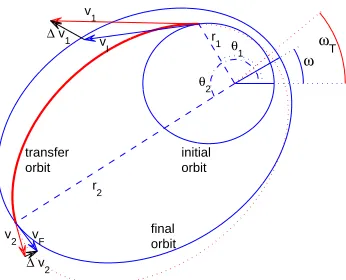
ω ωT
initial orbit transfer
orbit
final orbit
r
1 θ 1
r
2
θ2
v
I
∆ v
1
v
1
vF v2
∆ v
[image:5.595.91.264.134.274.2]2
Figure 1: Geometry of the orbit transfer
The parameters to be set for the MOPED algorithm are: size of the population,Nind, number of constraint classes,Ncl, the fitness coefficient,α, the sampling pro-portion,τ.
3. Problem Statement
3.1 Geometry, Objectives and Constraints
The geometry of a generic two–impulse coplanar orbit transfer is depicted in Fig. 1. Both the initial and the target orbits are defined by means of their orbital elements, indicated by the subscript I and F, respec-tively. Problem geometry is defined by 6 quantities only, namely semi–major axis,aI andaF, eccentricity,
eI andeF, angle between the periapsis, ∆ω, and initial spacecraft position on the initial orbit, θσ0. Assuming the periapsis of the initial orbit as reference for angles, the argument of the periapsis for the initial and target orbits areωI= 0 anωF = ∆ω, respectively.
The transfer is accomplished by means of two im-pulses, ∆~v1 and ∆~v2, identified by their magnitude ∆v=||∆~v||and angle with respect to the tangential direction,φ. The first impulse at timet1=tW (where
tW indicates the waiting time on the initial orbit) in-jects the spacecraft on the transfer orbit (thick line in Fig. 1); the second one at timet2=tF =t1+tT(where
tTis the transfer time) injects the spacecraft on the tar-get orbit and completes the prescribed maneuver. The parameters of the transfer orbit will be identified by the subscriptT.
If the initial orbit is circular, its periapsis is not de-fined and the periapsis of the target orbit is assumed as reference for the anomalies. If both orbits are circular, as for the Hohman transfer case, the problem is sym-metric and the spacecraft position at injection time has
no influence on the transfer, so thatt1= 0 andθσ0= 0 are assumed without loss of generality.
In all the considered cases, one of the objective func-tions is the total velocity increment, namely
∆vtot = ||∆~v1||+||∆~v2||
The total transfer time, given by the sum of waiting and transfer times,tF, is included in the analysis as the sec-ond merit function, for multi–objective optimization. If a rendez–vous problem is dealt with, a further problem parameter is the target position at the initial time,θτ0. In such a case a constraint on the final spacecraft po-sition is represented by the conditionθσ2=θτ2, where the subscriptsσ andτ indicate spacecraft and target, respectively.
Other constraints are included in the analysis. In particular, only arcs of elliptic orbits will be consid-ered as admissible transfer trajectories, so that a first constraint is
eT<1
When considering planet centered orbits, the transfer orbit must remain higher than a prescribed minimum over the surface. Such a condition is enforced by means of the inequality
rT ,min≥krPI,
whererT ,min is the minimum radius along the transfer orbit arc, while rPI = aI(1−eI) is the initial orbit periapsis and k ≤ 1 is a prescribed coefficient. Note that if the transfer orbit periapsis lies outside of the considered transfer arc, it is rT ,min = r1 ≥ rPI, and the constraint is not active.
3.2 Definition of benchmark cases
As stated in the Introduction, this preliminary analy-sis is focused more on the methodological aspects of the problem of comparing different optimization ap-proaches, including how the orbit transfer is repre-sented in the optimization process. For this reason, only relatively simple cases (two–impulse transfers be-tween circular and elliptical orbits, three–impulse trans-fer with rendez–vous on the target orbit and a simul-taneous two–impulse transfer for two formation–flying satellites) are considered as test benchmarks for the considered approaches. All the relevant data relative to these cases are summarized in Tab. 1. These cases are sufficient for outlining the major findings of this preliminary study. More complex scenarios will be the object of forthcoming research.
3.2.1 Case 1: Direct transfer between circular orbits
Table 1: Orbits for benchmark cases
Case No. of satellites Planet µ aI eI aF eF
1 1 Mars 4.2828 104 km3s−2 8 000 km 0 15 000 km 0
2 1 Earth 3.9860 105 km3s−2 6 721 km 0 26 610 km 0.667
3 1 Earth 3.9860 105 km3s−2 7 000 km 0 42 000 km 0
4 2 Earth 3.9860 105 km3s−2 7 000 km 0 42 000 km 0
solution can be derived analytically (the well–known Hohmann transfer, for the minimum–fuel problem [17]), this case was often used in the past as a preliminarily assessment of the capabilities of EAs in the framework of orbit maneuver optimization [18–20]. In particular, [18] and [19] represent two of the first examples of ap-plications of GAs to orbit maneuver problems, while [12] offers maybe the first attempt of comparing dif-ferent evolutionary approaches on the same problem, although in a relatively qualitative way.
The case considered, taken from [20], is the trans-fer between two circular Mars orbits of diftrans-ferent radii. As a difference with respect to the cited applications of GAs, both fuel consumption and trasfer time are as-sumed as objective functions to be minimized so that the Hohmann transfer represents one of the extremes of the Pareto front in the ∆vtot–tT plane.
Together with the constraint on the eccentricity of the transfer orbit, e < 1, the minimum distance con-straint is also enforced with k = 1. The geometry of the problem is defined by the ratio of the radii,rF/rI, and the waiting time has no influence on the transfer (including the optimal one), because of the radial sym-metry of the problem.
3.2.2 Case 2: Direct transfer with rendez–vous A slightly more complex case was considered by A. Re-ichert in her work [18], where transfers between generic elliptical orbits were also dealt with. Only if the el-lipses are aligned a Hohmann–like optimal transfer is easily determined. In the general case, the lines of the apsides of the two orbits form a certain angle, ∆ω, and the variation of ∆vtot as a function of the extremes of the transfer arc is more complex.
The geometry of the problem is described by a higher number of parameters, namely the ratio of the semi– major axes, aF/aI, the eccentricities, eI and eF, and the angle ∆ω. The solution depends on the initial spacecraft positions, θσ at time t= 0, even when the initial orbit is circular (e.g. a circular LEO), so that
eI = 0 and ∆ωis no longer defined.
In this paper, a further constraint is added on the fi-nal position, that is, the spacecraft must reach a target on the final orbit (rendez–vous problem). In this sce-nario the solution depends also on the initial position of the target, θτ at time t = 0. A further constraint
is introduced on the final position, θσ = θτ at time
t=tF ≡t2.
The data used for Case 2 and reported in Tab. 1 are representative of a transfer from a circular LEO to a high eccentricity semisynchronous orbit. The transfer depends on two parameters only, namely tW and tT. Figure 2 represents a contour plot of ∆vtot as a func-tion of these two parameters (white<3 m/s, black>15 m/s). The shaded areas represent unfeasible solutions where constraints on eccentricity and/or minimum ra-dius are violated. The variation of ∆vtot in thetW–tT plane is characterized by several local minima. As a consequence, the Pareto front in the ∆vtot–tT plane is expected to exhibit several arcs.
t W [h]
t T
[h]
0 2 4 6 8 10 12 14 16
[image:6.595.310.500.398.604.2]1 2 3 4 5 6 7 8
Figure 2: ∆vfor Case 2.
3.2.3 Case 3: Three–impulse transfer
Similar cases were also analyzed in [19] and [20], al-though for different geometries and, apparently, with the only purpose of demonstrating the possibility of generalizing the optimization approach to a genericn– impulse transfer. In the present application a constraint on the final position is considered, so that the inter-mediate velocity increment can be used to correct the trajectory along the path and make the rendez–vous with the target somehow easier. Constraints on the ec-centricity and minimum distance from the planet sur-face are enforced for both arcs, exactly as for the two– impulse transfer.
3.2.4 Case 4: Simultaneous transfer of 2 satellites A final more complex application is considered, where two formation–flying satellites, indicated by the letters
A and B are launched simultaneously from the same position on LEO towards two prescribed longitudes on GEO shifted by an angle ∆λ [12]. In this case the algorithm minimizes the total ∆vrequired by the for-mation, ∆vF F = ∆vtot,A+ ∆vtot,B, and the maneuver timetman, that is, the time at which the last spacecraft achieves its prescribed position,tman= max(t2,A, t2,B). As a matter of fact, two–impulse orbit transfers be-tween circular orbits is considered with the constraint that the initial position is the same for both satellites. Also the constraints considered for Cases 2 and 3 apply in the same form as before to both spacecraft.
3.3 Representation of Orbit Transfers
In this paragraph the functional dependencies of merit functions and constraints with respect to the un-knowns of the optimization problem will be expressed, in order to highlight the differences between the two considered representations of the orbit transfer problem for Keplerian motion: the first one, based on a standard orbit propagation algorithm (f-gmethod based on La-grangian coefficients); the second based on the solution of the Lambert problem.
In this latter case the required ∆v is obtained af-ter the solution of the Lambert problem as a function of the orbit parameters of the orbit that contains the transfer arc, while in the first case magnitude and di-rection of the velocity increment are among the opti-mization variables, while the final position and transfer time are obtained from orbit propagation. As a conse-quence number of optimization variables (that is, the dimension of the search space) and the representation (or even the presence) of constraints may vary, when describing the transfer in different terms, thus affecting the performance of the optimization algorithm used.
3.3.1 Orbit propagation
When orbit propagation is used for determining the op-timal two–impulse transfer, the optimization variables
are magnitude and direction of the velocity increment of the two impulses, namely ∆v1 and φ1 for the first impulse, and ∆v2andφ2for the second one (where the angleφiis counted with respect to the local tangent to the orbit), together with the orbital anomalies θ1 and
θ2=θ1+∆θof the corresponding positions. The vector of optimization variables is thus given by
x= (θ1,∆v1, φ1,∆θ,∆v2, φ2)T∈R6
A total of 5 constraints is enforced: 3 equality con-straints on semi–major axis, aF, eccentricity, eF, and argument of the periapsis,ωF, for the final orbit, and two inequality constraints for the transfer orbit, that is,
eT<1 andrmin> kaI(1−eI).
When a transfer between circular orbits is consid-ered (Case 1), the symmetry of the problem makes θ1 loose any influence on both the objective functions. For this reason the variable is assumed to be zero and the search space dimension is reduced to 5. All the other aspects of the optimization problem remain unchanged. A sixth constraint is added for the rendez–vous prob-lem (Case 2), in which case the spacecraft must achieve a prescribed position at the final time, after the sec-ond impulse. This requires that also the position of the target on the final orbit is propagated.
The extension to ann–impulse case (Case 3) simply requires that more optimization variables are added and the orbit propagation algorithm is appliedntimes. For the three impulse case (Case 3) it is
x= (θ1,∆v1, φ1,∆θ1,∆v2, φ2,∆θ2,∆v3, φ3)T ∈R9 withθi+1=θi+ ∆θi.
Inequality constraints apply to both arcs, so that a total o 4 inequality constraints need to be enforced, plus the usual three equality ones on the final orbit.
The simultaneous two–impulse transfer of two space-craft duplicates the number of optimization variable, with respect to Case 2, with the only exception of the starting point, which is common to both satellites. The vector of optimization variables is
x = (θ1,∆v1,A, φ1,A,∆v1,B, φ1,B,
∆θA,∆θB,∆v2,A, φ2,A,∆v2,B, φ2,B,)T∈R11 and 6 equality constraints plus 4 inequality constraints are enforced.
In all the above mentioned cases, each one of the equality constraints on orbit parameters and spacecraft final anomaly (rendez–vous condition) is enforced by means of two inequality constraints in the form
aF,des−εa≤aF ≤aF,des+εa
eF,des−εe≤eF ≤eF,des+εe
ωF,des−εω≤ωF ≤ωF,des+εω
whereεa,εe,εω, andεθ are the assumed tolerances. 3.3.2 Lambert Problem
The solution of the two–point boundary value problem for Keplerian motion, also known as Lambert’s problem [17], is represented by the determination of the orbit parameters of an orbit having a specified transfer time
tdes between two prescribed positions in space,P1 and
P2. Several algorithms have been derived for solving it, from the seminal works of prof. R.H. Battin [22] to a recent algorithm developed by G. Avanzini (see [3] and references therein).
Most of the methods are based on a parameterization of the set of orbits passing troughP1 and P2 with re-spect to some auxiliary variable. The method described in [3] exploits a novel parametrization in terms of the transverse eccentricity vector componentet, perpendic-ular to the direction of the chord connectingP1andP2. As far as the transfer timetT is a monotonic function ofet, the latter is used as the unknown for the equation
tT(et) =tdes.
It should be noted that, when a Lambert algorithm is used for defining the geometrical properties of either a two–impulse transfer orbit or the last trajectory arc for then–impulse case, the constraints on the final position of the spacecraft at the end of the transfer are inher-ently satisfied, and the required ∆~v’s are identified by simple vector operations as
∆~v1 = ~v1−~vI ∆~v2 = ~vF −~v2
where the initial and final velocities ~vI and ~vF are known from the properties of the (given) initial and final orbits, while~v1 and~v2 are determined from the orbital elements of the transfer arc.
This fact greatly simplifies the structure of the feasi-ble solution space, inasmuch as, together with the num-ber of equality constraints, also the numnum-ber of optimiza-tion variables is reduced. This is done at the expenses of a higher computational cost for the evaluation of a single individual of the population of candidate solu-tions, which requires the iterative solution of the Lam-bert problem for the considered set of transfer param-eters (starting and arrival positions on the initial and final orbits and transfer time).
For Case 1 the problem is almost over–simplified, the number of optimization variables being reduced to only two, that is,
x= (∆θ, tT)T∈R2
withθF = ∆θ. Also Case 2 can be easily cast in a form where only two optimization variables are present,
x= (tW, tT)T ∈R2
If on one side, the transfer between elliptical orbits de-pends on the waiting time on the starting orbit, the ad-ditional rendez–vous constraint dictates the final posi-tion at the end of the transfer, where the target posiposi-tion at the final timetW+tT is easily found from the knowl-edge of its initial position at timet= 0 by application of an orbit propagation algorithm. As a matter of fact, in both these first two cases, the Pareto front could be directly traced with very simple numerical techniques. For the three–impulse transfer (Case 3) the search space is spanned by the vector
x= (tW, tT1, r1,∆θ1, tT2)T ∈R5
where r1 and ∆θ1 assign the position of the interme-diate impulse, whiletT1 andtT2 are the transfer times along the first and the second coast arc, respectively.
On the converse, the vector of optimization variables for the simultaneous transfer of two spacecraft (Case 4) is
x= (tW, tT A, tTB)
T ∈R3.
For all the above mentioned cases, inequality con-straints on eccentricity and minimum radius apply to transfer orbit segments as before, but all the equality constraints are now exactly satisfied by the problem representation itself. Although inequality constraints reduce the size of the admissible region in the search space, the subset of feasible solutions has the same di-mension of the search space. A very different situation is encountered when orbit propagation is used for rep-resenting the transfer. As an example, Case 4 is char-acterized by 11 unknown and 8 constraints, resulting in a three–dimensional subset of feasible solutions in a 11–dimensional search space.
4. Test Methodology
The optimization algorithms adopted in this work be-long to the wide class of stochastic algorithm. These methods are expected to converge to the global solu-tion of the problem if the number of evaluasolu-tions of the system model Neval is sufficiently high. Equivalently, lettingPsbe the probability to find the global solution,
4.1 Comparison metrics
All the benchmark problems considered in this work are constrained and multi-objective. Therefore the perfor-mance of the algorithms must be measured in terms of constraint satisfaction and approximation of the global Pareto front.
A first index gives information about the capability of the algorithm of finding at least one feasible solu-tion. Given the total number of runs for the algorithm,
Nrun, the index PF S is the ratio between the number of times the algorithm is able to find at least one fea-sible solution, NrunF, and the total number of runs:
PF S=NrunF/Nrun.
As for the two main goals of MOEAs, that is, (i) convergence to the true Pareto optimal front, and (ii) distribution of the population over the whole front, it is necessary to introduce two parameters that evaluate both these properties. In this work, the metrics pro-posed by M. Vasile were adopted [23]:
Mconv = 1 Np Np X i=1 min j∈Mp 100
˛ ˛ ˛ ˛ ˛ ˛ ˛ ˛
gj−fi
gj ˛ ˛ ˛ ˛ ˛ ˛ ˛ ˛ (1)
Mspr =
1 Mp Mp X j=1 min i∈Np 100
˛ ˛ ˛ ˛ ˛ ˛ ˛ ˛
fi−gj
gj ˛ ˛ ˛ ˛ ˛ ˛ ˛ ˛ (2)
Given theMpsolutionsgjused to describe (or to ap-proximate) the global Pareto front, and theNpelements
fiin the Pareto front obtained from a given run of the optimization algorithm,Mconvis the sum overNpof the distance of each element in the particular front consid-ered from the closest element of the global front. This figure of merit clearly indicates how close the obtained front is to the global one. On the other hand,Mspr is the sum over all the elements in the global Pareto front of the distance of each element in the global front from the closest one in the front obtained for the considered run. This parameter measures how well the individuals of the obtained front cover the whole global front.
MconvandMsprcan assume different values for each run. A Gaussian PDF is usually assumed for these pa-rameters, described by mean value and variance, com-puted by taking into account only those runs that have at least one individual in the feasible region.
4.2 Integral approach for comparison metrics
The aggregated form briefly described above reflects the common practice for the evaluation of performance indexes of stochastic algorithms, but it has a signifi-cant methodological and practical fault that needs to be underlined, because thea priori hypothesis that the PDFs are Gaussian is usually far from true. The ac-tual PDF depends on a) the considered problem, b) the algorithm and c) the value ofNM AX. Its shape is
unknown and it can be multi–modal. As an example, both multi–objective performance indexes,Mconv and
Mspr, would be 0 at convergence, forNM AX→ ∞, with a PDF represented by a Dirac function centered in zero. For NM AX <∞both metrics are strictly positive by definition, so that, for very high values of NM AX one expects a PDF more similar to an exponential than a Gaussian one. Only for relatively low values ofNM AX the values of Mconv and Mspr will be distributed on both sides of the most likely one.
For this reason, in the absence of any actual knowl-edge about the true shape of the PDF, a practical and useful, yet correct and rigorous approach is based on extracting from the test results the success probabil-ity, which is the probability that the considered in-dex is beyond a predefined threshold. As an exam-ple, PS(Mconv < θconv) is the probability that the index Mconv achieves a value less than the threshold
θconv. These probabilities can be evaluated over a lim-ited number of runs with a better confidence then the PDF could be, so that it provides a more reliable merit function for optimization algorithm capabilities.
At this point, two indexes of success,PF S,Mconv and
PF S,Mspr, can be derived by combining constraint sat-isfaction probability and multi–objective requirements, that is:
PF S,Mconv = PF SPS(Mconv< θconv) (3)
PF S,Mspr = PF SPS(Mspr< θspr) (4) The first one is the product of the probability to find at least one solution in the feasible region times the probability that the indexMconv has a value less than the threshold θconv. If one assumes that Mconv = ∞ for those runs which are not able to find feasible so-lutions,PF S,Mconv is equivalent toPS(Mconv < θconv) computed on the basis of the whole set of runs. 4.3 Critical aspects and practical solutions
In order to compute the two multi-objective metrics,
Mconv and Mspr, the knowledge of the global front is required, either in analytic form or as a large set of global solutions. At the moment, such an information is not available, but it is possible to extract the best approximation of the global front from the whole set of available solutions, to be used as the reference global front.
knowing a priori the relation between the number of runs,Nrun, and the error on the estimation of the suc-cess index.
A commonly adopted starting point for sizing the sample of a binomial distribution is to assume that both the normal approximation for the sample proportionp
of successes (i.e. p ∼ N{θp, θp(1−θp)/n}, where θp is the unknown true proportion of successes) and the requirement that P r[|p−θp| ≤ derr|θp] are at least equal to 1−αp[24]. This leads to expression:
Nrun≥θp(1−θp)χ2(1),αp/d 2
err (5) that can be approximated conservatively with
Nrun≥0.25χ2(1),αp/d 2
err (6)
valid forθp= 0.5.
In the framework of this preliminary test campaign, relatively modest computational resources were avail-able, so that the above relations could not be used to size Nrun on the basis of an acceptable error level. Rather, the same relations were used in order to es-timate the error on the evaluation of the considered probability forNrun= 20. From Eq. 6 one has:
derr≥
q
0.25χ2
(1),αp/Nrun (7) For Nrun = 20, with a 95% confidence level (αp = 0.05), the measured success index can be affected by an error as high asderr&0.15.
5. Results
In order to allow for a fair and easy comparison be-tween the two optimization codes over the considered cases, code parameters were kept fixed, whenever pos-sible. For the NSGA-II code, the following values were adopted: crossover probability, pc = 0.9; mutation probability,pm= 1/dim(wheredim is the dimension of the search space); distribution indexes for crossover and mutation, ηc = 5 andηm = 5, respectively (val-ues that should allow a good exploration of the search space).
For the MOPED code the parameters were: number of constraint classes,Ncl= 10%Nind; fitness coefficient,
α= 0.5; sampling proportion,τ = 1.
For both codes, Nind and the maximum number of generations were set for each case on the basis of the expected degree of difficulty.
All the results in terms of performance indexes are listed in Table 2. Each particular case will be de-tailed and commented separately in the next subsec-tions. Only at the end, general properties and specifi-cations will be discussed.
5.1 Transfer between circular orbits
[image:10.595.345.460.250.353.2]The first and easiest test case was approached by Lam-bert method usingNind= 100 andNgenM AX = 20, for a total of 2000 evaluations of the system model, with following parameters and related bounds: x1 is the ∆θ of the transfer arc (x1 ∈[0.1,2π−0.1]),x2 is transfer time (x2∈[0.05, TF], whereTF is the period of the des-tination orbit). The minimum-fuel solution obtained by Lambert approach is shown in Figure 3.
Figure 3: Min–fuel transfer manoeuvre for Case 1.
0 1 2 3 4 5 6 7
0 1 2 3 4 5 6
∆ v
Ttot
PROP LAMB
Figure 4: Best reference Pareto fronts for Case 1.
As for all the other test cases by Lambert method, both the algorithms always successfully find the feasi-ble region, PF S = 1, and in this particular case they apparently have the same effectiveness in covering the whole front. On the other hand, there is an appre-ciable difference in terms of convergence onto the best front. The whole reference front, reported in Fig. 4, is better approximated over its whole extension by the solution reported in Fig. 5, whereMspr ≈1, then in Fig. 6, where the reported solution is characterized by
Mspr>2.
[image:10.595.314.493.411.556.2]ad-Table 2: Performance indexes - For all of the cases: Nrun= 20,θconv= 0.35,θspr= 1.25
¯
Mconv σ2(Mconv) M¯spr σ2(Mspr) PF S PS,Mconv PS,Mspr PF S,Mconv PF S,Mspr
Case 1.L
MOPED 0.245 0.0023 1.62 0.122 1 1 0.15 1 0.15
NSGA2 0.378 0.0073 1.48 0.067 1 0.35 0.2 0.35 0.2
Case 1.P
MOPED 0.19 0.02 6.2 2.11 0.95 0.89 0 0.85 0
NSGA2 61.41 9996.34 88.61 10595.66 0.2 0.25 0 0.05 0
Case 2.L
MOPED 0.07 0 5.8 15.21 1 1 0 1 0
NSGA2 0.09 0 2.04 0.14 1 1 0 1 0
Case 2.P
MOPED 0.3 0.01 0.58 0.06 1 0.8 1 0.8 1
NSGA2 110.5 11316.4 493.56 117304.3 0.55 0 0 0 0
Case 3.L
MOPED 20.52 165.24 5.553 2.451 1 0 0 0 0
NSGA2 4.68 27.62 4.88 27.36 1 0.2 0.25 0.2 0.25
Case 3.P
MOPED 42.84 5048.54 115.13 20814.72 0.65 0.15 0 0.1 0
NSGA2 18.35 465.67 61.92 2632.77 0.65 0.31 0 0.2 0
Case 4.L
MOPED 0.359 0.0026 1.19 0.00943 1 0.45 0.75 0.45 0.75
NSGA2 0.443 0.0035 1.21 0.046 1 0.05 0.65 0.05 0.65
Case 4.P
MOPED 5.68 62.27 34.61 735.7 0.8 0.5 0 0.4 0
NSGA2 NaN NaN NaN NaN 0 0 0 0 0
0 1 2 3 4 5 6 7
0 1 2 3 4 5 6
∆ v
Ttot
best reference single run
Figure 5: Run with Mspr = 1.066 < θspr = 1.25 for Case 1. lambert
ditional constraints (in this case εa = 20 km, εe = 0.005, and εω = 0.02 rad), it was approached with
Nind= 200 andNgenM AX = 400, for a total of 80000 evaluations of the system model. The bounds on the search variables were as follows: magnitude of the first impulse: x1 ∈ [0.02,1]; direction of the first im-pulse: x2 ∈ [−0.2π,0.2π]; position of the second im-pulse: x3 ∈ [0.2π,2π]; magnitude of the second im-pulse: x4 ∈ [0.02,1]; direction of the second impulse:
x5∈[−0.6π,0.6π].
0 1 2 3 4 5 6 7
0 1 2 3 4 5 6
∆ v
Ttot
best reference single run
Figure 6: Run with Mspr = 2.128 > θspr = 1.25 for Case 1. lambert
[image:11.595.77.516.152.403.2]5.2 Transfer Between Elliptical Orbits with Rendez-vous
A first more demanding test for the considered algo-rithms is represented by the optimization of orbit trans-fer between elliptical orbits, when a prescribed target on the final orbit has to be reached at the end of the maneuver. In this case, when the Lambert formulation is used, the algorithms where set withNind= 100 and
NgenM AX = 20, for a total of 2000 evaluations of the system model, with the following parameters and re-lated bounds: waiting time (tW =x1 ∈[0,10.8; trans-fer time: tT =x2∈[0.03,10.8].
[image:12.595.82.265.519.658.2]Both the algorithms demonstrate to be able to con-verge to the best front, but none of them can spread the individuals over the whole front. In Figure 7 the minimum-fuel solution obtained by Lambert approach is shown.
Figure 7: Min–fuel transfer manoeuvre for Case 2.
2 4 6 8 10 12 14
0 2 4 6 8 10
∆ v
Ttot
PROP LAMB
Figure 8: Best reference Pareto fronts for Case 2.
When the same case is modeled in terms of orbit propagation, the resulting optimization problem proved again to be more complex to solve. Given the additional
constraints,εa= 40 km,εe= 0.002,εθ= 0.01 rad, and
εω = 0.01 rad, Nind= 200 andNgenM AX = 600 were used, for a total of 120000 evaluations of the system model. The optimization parameters were bounded as follows. Position of the first impulse: x1∈[−0.2π,14π]; magnitude of the first impulse: x2 ∈[1.6,4]; direction of the first impulse: x3 ∈[−0.2π,0.2π]; position of the second impulse: x4 ∈[0.2π,2π]; magnitude of the sec-ond impulse: x5 ∈ [0.004,1.6]; direction of the second impulse: x6∈[−0.6π,0.6π].
Again for this constrained case the difference tween the performance of the algorithms is evident, be-ing much higher than the expected error derr both in terms ofPF S andPS,Mconv, but in the present case the MOPED algorithm successfully spreads the solutions along the front.
5.3 Three–impulse transfer
The three–impulse transfer with target on the final orbit is one of the two more complex cases handled. The version with the Lambert formulation, significantly more complex than the first two cases, was approached with Nind = 100 and NgenM AX = 300. The opti-mization variables were: the waiting time, tW =x1 ∈ [0,1.62); the transfer time for the first arc, tT ,1 =
x2 ∈ [0.03,21.54]); the radius of the second impulse,
r2 = x3 ∈ [7010,105410]); the amplitude of the first transfer arc (∆θ=x4∈[0.01,2π−0.01]); and the trans-fer time for the second arc (tT ,2=x5∈[0.03,21.54]).
Figure 9: Min–fuel transfer manoeuvre for Case 3.
0 5 10 15 20
0 2 4 6 8 10 12 14
∆ v
Ttot
PROP LAMB
Figure 10: Best reference Pareto fronts for Case 3.
When the same case is modeled by orbit propaga-tion, the constraints are enforced with the following tolerances: εa = 140 km, εe = 0.002, εθ = 0.01 rad, and εω = 0.01 rad, while Nind = 500 and
NgenM AX = 1200, for a total of 600000 evaluations of the system model. The position of the first impulse was bounded asx1∈[−2π/100,2π]); the magnitude of the first impulse was x2 ∈ [0.6,3], while its direction was
x3 ∈[0,0.2π]; the second impulse, delivered in a posi-tionx4 ∈[2π/100,2π]), had magnitudex5 ∈[0.003,3] and direction x6 ∈ [−0.4π,0.4π]; the third impulse was delivered in position x7 ∈ [2π/100,2π], with a magnitude equal to x8 ∈ [0.003,3] and a direction
x9∈[−0.6π,0.6π]).
[image:13.595.310.492.336.474.2]In this case the indices demonstrate comparable per-formance, although a mild prevalence of NSGA-II algo-rithm must be recognized. It should also be noted that none of the algorithms covers the whole reference front, for the considered sets of algorithm parameters.
Figure 11: Min–fuel transfer manoeuvre for Case 4.
5 10 15 20 25 30 35
0 2 4 6 8 10
∆ v
Ttot
PROP LAMB
Figure 12: Best reference Pareto fronts for Case 4.
5.4 Simultaneous transfer of 2 satellites
Case 4 with Lambert formulation was approached with
Nind= 100 andNgenM AX = 100 and with the following parameters: waiting time tW =x1 ∈ [0,1.62; transfer time for the first satellite tT ,A = x2 ∈ [0.03,21.54]; and transfer time for the second satellite (tT ,B =x3∈ [0.03,21.54]).
The algorithms appear equivalent in terms of both
PF S andPS,Mspr, but MOPED looks superior in terms of PS,Mconv. In Figure 9 the minimum-fuel solution obtained by the Lambert approach is shown.
When the case is modeled by a propagation method,
the position of the second impulse for satellite A is
x4 ∈ [2π/100,2π]; its magnitude x5 ∈ [0.003,2.7]), while its direction is x6 ∈ [−0.6π,0.6π]; the magni-tude of the first impulse for satellite B is x7∈[1.5,3], with direction x8 ∈ [0,0.2π]; the position of the sec-ond impulse for satellite B is x9 ∈ [2π/100,2π], with a magnitude equal tox10∈[0.003,2.7] and a direction
x11∈[−0.6π,0.6π].
In this case a comparison is not possible because none of the 20 runs of the NSGA-II provided any feasible solution. The result is somehow unexpected and will be investigated.
5.5 Remarks and comments
There are few comments and remarks that need to be pointed out. First of all, it appears evident from the tests that an approach by propagation method is not the best choice. Compared to the the Lambert ap-proach, propagation requires to handle a higher num-ber of design variables and constraints and, even if the MOPED algorithm appears capable of always reaching the feasible region, the optimization approach becomes extremely expensive.
Also, discrepancies between the best reference fronts obtained by the two modeling approaches demonstrate two major findings of this research: a) constraints, es-pecially for more complex cases, tend to bias the search towards a relatively limited portion of the feasible re-gion of the search space; this means that the coverage of the entire front in one run becomes unlikely and, since our reference fronts are the union of relatively few runs, they are not even complete; b) ideally, in order to find a truly global solution of the problem, the search for all the design variables should be allowed to vary be-tween−∞and∞; this was not done, in order to avoid regions where the model is not valid and to limit the computational time, but in such a way it is not easy to provide the considered approaches with exactly equiv-alent search spaces.
A second observation concerns the unquestionable superiority of the Lambert approach. Even if it can be considered as demonstrated, the presented results can only be seen as “qualitative” and “relative”, because of the relatively small number of test runs for each case. The aim of this work was to provide new ideas for future extensive tests, that, based on a wider range of results, will allow for a more correct interpretation of the data. At present the obtained index values are affected by the following problems:
• a low value ofNrun, in this case, influences twice the precision of the results: a) a high value ofderr allows to distinguish between the algorithms only when the discrepancy in terms of indexes is very high; b) the best Pareto front is itself a product
of the runs, therefore also the confidence on the reference front is low whenNrunis small; • sinceθconvandθsprare fundamental for the
deter-mination of the merit index, a standard value for all of the cases may not be the best choice. Part of the future work will be aimed at standardiz-ing the models, both in terms of variable bounds and constraint levels (ǫa, ǫe, ǫθandǫω), in order to use them as benchmarks for constrained optimization algorithms.
6. Conclusions and Future Work
An approach for comparing performance of Evolu-tionary Optimization Algorithms has been developed and tested over a set of 4 benchmark case, using two dif-ferent multi–objective optimization codes: a standard genetic algorithm and a Parzen–based estimation of dis-tribution algorithm. Two different representation of the orbit transfer problem were also adopted, for a total of 4 possible different optimization approaches. With re-spect to the second are-spect, modeling the transfer orbit by solving a Lambert problem allows for a direct en-forcement of constraints on the final position (includ-ing rendez–vous), which greatly simplifies the solution of the optimization problems, by reducing the number of optimization variables at stake. At the same time, orbit propagation still offers a good benchmark for test-ing the capabilities of different algorithms over con-strained problems. As for the optimization codes, the adopted version of MOPED algorithm performs usually better than the adopted version of NSGA-II, although the limited number of runs available makes this state-ment somehow questionable and the comparison only qualitative.
In this respect, considering the proposed comparison metrics for multi–objective optimization as representa-tive of the actual performance of the algorithms, future research will be addressed towards improving (i) the evaluation of the statistical properties of the perfor-mance indices adopted, by means of a higher number of runs, and (ii) the standardization of the test cases, by making the search space truly equivalent.
References
1. K. Deb,Multi-Objective Optimization Using
Evo-lutionary Algorithms. John Wiley & Sons, NY,
2. M. Costa, E. Minisci, “MOPED: a Multi-Objective Parzen-based Estimation of Distribu-tion algorithm”, Second InternaDistribu-tional Confer-ence on Evolutionary Multi-Criterion Optimiza-tion, EMO 2003, Faro, Portugal. Springer - LNCS 2632. 2003, pp. 282–294
3. G. Avanzini, “A Simple Lambert Algorithm”, J. Guid. Control & Dyn., Vol. X(5), 2008, in print.
4. L. Casalino, G. Colasurdo, and D. Pastrone, “Indirect approach for minimum-fuel aeroassisted transfers,” AIAA/AAS Astrodynamics Confer-ence, San Diego, CA, July 1996, AIAA Paper 96– 3592.
5. M. La Mantia, and L. Casalino, “Indirect Opti-mization of Low-Thrust Capture Trajectories,”J. Guid. Control & Dyn., 29(4), 2006, 1011–1014.
6. C.L. Ranieri, and Cesar A. Ocampo, “Indirect Optimization of Two-Dimensional Finite Burning Interplanetary Transfers Including Spiral Dynam-ics,”J. Guid. Control & Dyn., 31(3), 2008, 720– 728.
7. D.P. Bertsekas, Constrained Optimization and
Lagrange Multiplier Methods, Athena Scientific,
1996.
8. T. B¨ack,Evolutionary Algorithms in Theory and Practice: Evolution Strategies, Evolutionary
Pro-gramming, Genetic Algorithms, Oxford Univ.
Press. 1996.
9. M. Mitchell. An introduction to genetic
algo-rithms, MIT Press, 1998.
10. H.G. Beyer, and H.P. Schwefel, “Evolution Strate-gies: A Comprehensive Introduction”, Journal Natural Computing, 1(1):3-52, 2002.
11. K.V. Price, R.M. Storn, and J.A. Lampinen.
Dif-ferential Evolution. A Practical Approach to
Global Optimization. Natural Computing Series,
Springer, 2005.
12. G. Avanzini, E.A. Minisci, and D. Biamonti, ”Minimum-Fuel/Minimum-Time Maneuvers of Formation Flying Satellites”, AAS/AIAA Astro-dynamics Specialist Conference, Big Sky, Montana (USA), August 2003. AAS Paper 03-654.
13. C.R. Bessette, and D.B. Spencer, “Performance Comparison of Stochastic Search Algorithms on the Interplanetary Gravity-Assist Trajectory Problem,” J. Spacecraft & Rockets, 44(3), 2007, 722-724.
14. P.L. Di Lizia, G.M. Radice, D. Izzo, M. Vasile, “On the Solution of Interplanetary Trajectory De-sign Problems by Global Optimisation Methods”, Proceedings of GO 2005, pp. 1–7.
15. M. Vasile, E. Minisci, and M. Locatelli, ”On Test-ing Global Optimization Algorithms for Space Trajectory Design”, AIAA/AAS Astrodynam-ics Specialist Conference and Exhibit, Honolulu, Hawaii (USA), August 2008, AIAA paper 2008-6277.
16. K. Deb, A. Pratap, S. Agarwal, and T. Meyarivan, “A Fast and Elitist Multiobjective Genetic Algo-rithm: NSGA-II”, IEEE Transactions on Evolu-tionary Computation, 6(2), April 2002.
17. R.H. Battin, An Introduction to the
Mathemat-ics and Methods of AstrodynamMathemat-ics, Revised Ed. ,
AIAA Education Series, Reston, Virginia (USA), 1999, Chpts. 4, 5.
18. A.K. Reichert, “Using a Genetic Algorithm to De-termine the Optimum Two-Impulse Transfer Be-tween Co-Planar, Elliptical Orbits,” inIndustrial Applications of Genetic Algorithms, C.L. Karr and L.M. Freeman editors, CRC Press, Boca Raton, FL (USA), 1999, pp. 111–133.
19. Y.H. Kim, and D.B. Spencer, “Optimal Spacecraft Rendezvous Using Genetic Algorithms,”J. Space-craft & Rockets, 39 (6), 2002, 859–865.
20. O. Abdelkhalik, and D. Mortari, “N-Impulse Orbit Transfer Using Genetic Algorithms,”J. Spacecraft & Rockets, 44(2), 2007, 456–459.
21. N. Khan, D.E. Golberg, and M. Pelikan, “Multi-objective Bayesian Optimization Algorithm”, Technical Report IlliGAL 2002009, University of Illinois at Urbana-Champain - IlliGAL, 2002. 22. R.H. Battin, “An Elegant Lambert Algorithm,”J.
Guid. Control & Dyn., 7(6), 1984, 662–670.
23. M. Vasile, “Hybrid Behavioural-Based Multiob-jective Space Trajectory Optimization”, on
Multi-Objective Memetic Algorithms, Springer Series of
Studies in Computational Intelligence, 2008, to ap-pear.