Novel numerical optimisation of the Hohmann Spiral Transfer

IAC-12-C1.6.7 Page 1 of 11 IAC-13-C1.6.7

NOVEL NUMERICAL OPTIMISATION OF THE HOHMANN SPIRAL

TRANSFER

Steven Owens

Advanced Space Concepts Laboratory/University of Strathclyde, Glasgow, Scotland,

[email protected]

Malcolm Macdonald

Advanced Space Concepts Laboratory/University of Strathclyde, Glasgow, Scotland,

[email protected]

__________________________________________________________________________________

As the revenue of commercial spacecraft platforms is generated by its payload, of which the capacity is maximised when fuel-mass is minimised, there is great interest in ensuring the fuel required for the trajectory to deliver the satellite to its working orbit is minimum. This paper presents an optimisation study of a novel orbit transfer, recently introduced by the authors through an analytical analysis, known as the Hohmann Spiral Transfer . The transfer is analogous to the bi-elliptic transfer but incorporating high and low-thrust propulsion. This paper has shown that substantial fuel mass savings are possible when utilizing the HST. For a transfer to Geostationary Earth Orbit it is shown that a fuel mass saving of approximately ( ) is possible for a wet mass of – whilst satisfying a time constraint of 90 days. Several trends in the gathered data are also identified that determine when the HST with high or low-thrust plane change should be used to offer the greatest fuel mass benefit.

__________________________________________________________________________________

I.NOMENCLATURE

g – standard gravitational acceleration, m/s2

µ - gravitational constant, km3/s2

mdry – spacecraft mass without fuel, kg

mwet – spacecraft mass with total fuel, kg

ΔVH(C/E) – high-thrust only system velocity

requirement (circular/elliptical initial orbit), m/s

ΔVHSTH(C/E) –HST high-thrust phase velocity

requirement (circular/elliptical initial orbit), m/s

ΔVHSTL – HST low-thrust phase velocity

requirement, m/s

IspH – high-thrust system specific impulse, s

IspL – low-thrust system specific impulse, s

ΔV – total velocity requirement, m/s

ΔVi – velocity requirement to transfer between

specified orbits, m/s

ΔVf – velocity requirement to transfer between

specified orbits, m/s

υi – initial orbit velocity at beginning of specified

transfer, m/s

υf – target/intermediate orbit velocity at end of

specified transfer, m/s

υt1– transfer orbit velocity at node associated with

initial orbit, m/s

υt2– transfer orbit velocity at node associated with

final orbit, m/s

ΔI – total plane change, radians

s –plane change at specified node, %

Tr – spacecraft thrust, mN

a – semi-major axis, m

p – semi-latus rectum, m

e – eccentricity

i – inclination, radians

υ – true anomaly, radians

ω – argument of perigee, radians

E – eccentric anomaly, radians

rp – radius of perigee, m

IAC-12-C1.6.7 Page 2 of 11

r – Instantaneous radius of spacecraft

ri – initial orbit perigee radius, m

rt – target orbit radius, m

rc – intermediate orbit apogee radius, m

rX – intermediate orbit perigee radius, m

R1 – target /initial perigee orbit ratio

R2 – intermediate apogee/initial perigee orbit ratio

f – modified equinoctial element

h – modified equinoctial element

g – modified equinoctial element

L – modified equinoctial element

τ – auxiliary positive variable

t – time, days

tMAX – maximum allowable transfer time, days

f– force, N

λσ– locally optimal orientation vector for element σ

̂ – locally optimal orientation unit vector for element σ

λb– locally optimal orientation blended vector

̂ – – locally optimal orientation blended vector

Wσ– optimized weighting constant for each element

σ

Figure Acronyms

HST HT C – Hohmann Spiral Transfer (HST) with high-thrust plane change, circular initial orbit

HST HT E – Hohmann Spiral Transfer (HST) with high-thrust plane change, elliptical initial orbit

HST LT C – Hohmann Spiral Transfer (HST) with low-thrust plane change, circular initial orbit

HST LT E – Hohmann Spiral Transfer (HST) with low-thrust plane change, elliptical initial orbit

II.INTRODUCTION

As commercial satellites have an ever-increasing role in our everyday lives, there is great demand for more satellite platforms to accommodate the services offered such as telecommunications, Global Positioning System (GPS) and Earth-monitoring. As the revenue of such platforms is generated by its payload, of which the capacity is maximised when fuel-mass is minimised, there is great interest in ensuring the fuel required for the trajectory to deliver the satellite to its working orbit is minimum. This paper presents an optimisation study of a novel orbit transfer, recently introduced by the authors through an analytical analysis, known as the Hohmann Spiral Transfer (HST). The transfer is analogous to the bi-elliptic transfer but incorporating high and low-thrust propulsion. The high-thrust system is used to propel the spacecraft beyond the target orbit to an intermediate orbit where the low-thrust system is activated and used to direct the spacecraft on a spiral trajectory in-toward the target orbit.

IAC-12-C1.6.7 Page 3 of 11

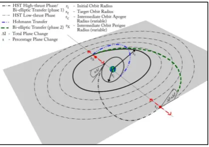
Figure 1 HST with varying intermediate orbit apogee and perigee. Hohmann and bi-elliptic transfers are also shown

III. HST ANALYTICAL METHOD

Several papers published by the authors [1-4] have developed the analytical analysis of the HST. This involved the generation of critical specific impulse ratios, which determine the system performance requirements to ensure the fuel mass of the HST is equal to that of the compared transfer (Hohmann or bi-elliptic). The critical ratios are derived from the fuel mass fractions of each transfer with the final form of the equation given in Eq. (1).

_{( ) ( )} (1)

Using these critical ratios, it is therefore possible to identify a fuel mass benefit using the HST. As for any mission, the target and initial orbits are known, as well as the inclination between these two orbits. This means there is only one variable remaining in the critical specific impulse ratio: the intermediate orbit radius, (the analytical constraint assumes this to be a circular orbit). In order to therefore introduce a fuel mass benefit, one or both of the following methods can be employed:

1. Increase the specific impulse ratio of the system i.e. improve the performance of the low-thrust system.

2. Increase the intermediate orbit radius, , which in turn reduces the critical specific impulse ratio (the general trend of the function is to decrease with increasing .)

In general, the larger the spacecraft specific impulse ratio compared to the critical specific impulse ratio, the greater the fuel mass benefit.

IV. HST NUMERICAL METHOD

The numerical method has been created for the main application of optimising the low-thrust section of the HST. However it can be modified to

include the high-thrust phase of the HST also. For this to work, it is assumed the high-thrust section is conducted through one or two impulsive burns. The first burn is used to enter the transfer orbit which takes the spacecraft beyond the target orbit. In the case where the low-thrust system is activated at the apogee of this orbit, this is the only high-thrust burn performed. In the case where the spacecraft enters an intermediate orbit at the apogee, a second high-thrust impulse is used to achieve this. It is worthwhile mentioning again that the analytical analysis assumed that the spacecraft enters a circular intermediate orbit at this far away point.

Low-Thrust Phase Methodology

Locally optimal control laws are used in the generation of the low-thrust phase of the HST within the numerical model. There are several locally optimal control laws which can be used to generate a trajectory, however as there are no orbit insertion requirements for the analysis in this paper only three or four control laws, depending on the optimisation problem, are required to conduct the trajectory calculation. Only three are utilised for the case where the HST employs a high-thrust plane change: the semi-major axis, eccentricity and radius of pericentre. The low-thrust section is therefore co-planar. For the case where the low-thrust system performs the plane change, the high-thrust phase is co-planar and the semi-major axis, eccentricity, inclination and radius of pericentre control laws are used to generate the low-thrust phase trajectory. If there are explicit mission constraints e.g. a specific insertion point on the geostationary belt, then additional control laws, including the argument of perigee and longitude of ascending node, can be used. By using only the minimum number of controls laws required to generate a trajectory ensures the software is optimized to suit the mission specification and the calculation time of the software is kept to a minimum.

Locally Optimal Control Laws

IAC-12-C1.6.7 Page 4 of 11

̂

where σ represents the respective element. The required force, in the Radial, Transverse and Normal Axes (RTN), to maximise the rate of change of σ, is a unit vector defined by By maximizing the force along , the instantaneous

rate of σ is also maximized. The variational equations are defined in Gaussian form as this allows each component of the perturbing acceleration to be identified[7,8].

Semi-Major Axis Control Law

The semi-major axis variational equation is given in Eq. (3) in classical elements.

√ [ ] [

]

By identifying and converting to modified equinoctial elements[9], the maximized direction vector is given in Eq. (4).

[ ]

[ ( ) ]

(4)

This can now be used to generate a locally optimal control law which focuses on maximizing the semi-major axis. This is also known as the energy gain control law as it gives a locally optimal variation in orbit energy.

Eccentricity Control Law

The eccentricity variational equation is given in Eq. (5) and is defined in classical elements.

[ ] [

] (5)

By identifying and converting to modified equinoctial elements, the maximized thrust direction vector is given in Eq. (6).

[ ] (6)

[

√ [ ][ ]

√

√

]

Radius of Pericentre Control Law

The radius of pericentre equation is given in Eq. (7) in classical elements. It can be seen that this variational equation is made up of both the semi-major axis and eccentricity equations.

( )

√ [ ] [

( )

( )( )

]

(7)

By identifying and converting to modified equinoctial elements, the maximized thrust direction vector is given in Eq. (8).

[

( ) ( )( )

]

[

[ ( √ ) _√ ]

( √ )( ) (

√ )

]

(8)

Inclination Control Law

The inclination control law varies to the previously defined. It depends only on the out of plane perturbation and as such a switching term is required in order to maintain the chosen rate of change, either positive or negative. It will change according to the argument of latitude. Eq. (9) gives the variational equation for inclination defined in classical elements.

√ [ ] [

( )] (9)

Identifying λi, converting to modified equinoctial

elements and applying the switching term as discussed, the maximized thrust direction vector is given in Eq. (10).

[

[ ( )]]

IAC-12-C1.6.7 Page 5 of 11

[

[ ( ) ( )]]

where √

Control Law Blending Method

As there are a maximum of four control laws involved in the trajectory generation process, each with their own maximized thrust vector, it is necessary to ‘blend’ these to generate a thrust vector that accommodates all the mission constraints. The blending method adopted for the numerical approach derives from a form of averaging that has previously been applied to solar sail trajectory design known as AnD (Accessibility and Deficit) blending[6,10]. The method is adopted here to suit low-thrust technologies without the limitations of a sail i.e. the thrust can be directed in any direction as and when it is needed. Several blending methods have previously been suggested: some which utilize weighting constants described as a function of time from the initial epoch[11,12]. The method used in this analysis is similar to the approach adopted by Petropoulos[13], which is independent of time and thus has the advantage of reduced simulation time as the weighting constants do not have to be calculated at every time-step.

The method used in this paper calculates the deficit (time to target) of each control law based on the maximized thrust vector if it were solely used and assuming a constant rate of change. These are normalized with respect to the largest, resulting with each control law receiving a score between zero and one: zero meaning the control law has achieved its target and one meaning it is furthest, in terms of time, from its target value. The control laws are then multiplied by an optimized weighting constant, , - discussed in detail in the optimization section - based on mission specification, before finally being blended using the averaging technique as is shown in Eq. (11). This now forms the maximized thrust direction vector; all symbols have the same meanings as previously discussed.

∑ ̂ ∑

where

(11)

High-Thrust Phase Methodology

As the numerical code is predominantly set up to accommodate low-thrust trajectory design, it is

necessary to modify it so that the high-thrust phase can be included to ensure this can also be optimized. The high-thrust phase is based on a ‘minimum energy’ two-impulse Hohmann transfer. For the case where the high-thrust phase also performs the plane change, it is assumed that this is split over the two impulse burns and conducted as a combined maneuver as is shown in Figure 1. This has been shown to be more fuel effective than performing each maneuver separately[14]. The method used to determine the optimal plane change split between the two impulses is described in the proceeding section. To ensure there is no unintended alteration to other orbital elements, it is assumed the line of nodes aligns with the major axis of the orbit.

It should be noted that this same plane change methodology is also applied to the compared transfer; Hohmann or bi-elliptic. For the bi-elliptic transfer, the velocity requirement is calculated for a plane change split across the first and second impulses as well as across the second and third impulses. For the case where the plane change is split across the first and second impulses, the third impulse is co-planar and similarly, for the case where the plane change is split across the second and third impulses, the first impulse is co-planar. The case where the plane change is split across the first and third impulses is not considered as it is assumed the second impulse should always be included as this is furthest from the central body and hence, should have a lower velocity requirement when performing the plane change. The case where the bi-elliptic performs the plane change over the first two impulses is shown in Figure 1, along with the Hohmann transfer.

Plane Change Split Methodology

In previous papers concerning the HST, the plane change split has been performed analytically to suit the analytical make-up of the paper[2,3]. Although the error associated with this was validated [15], this paper determines the optimal inclination split numerically using a Newton-Rhapson method[16]. To do this it is necessary to first determine the total velocity requirement of the high-thrust phase, including the plane change, as shown in Eq. (12). This is derived based on the law of cosines[17].

√ ( )

√ (( ) )

(12)

IAC-12-C1.6.7 Page 6 of 11 be partially differentiated with respect to and set

equal to zero to determine when the function is a minimum. The resultant function is shown in Eq. (13).

(( ) )

(13)

As appears on both sides, the newton rhapson method must be used to iterate and find a solution.

V. OPTIMIZATION METHOD

Algorithm

The optimization algorithm selected uses a constrained nonlinear optimization technique adapting a sequential quadratic programming (SQP) method. This is selected as it has a strict feasibility with respect to the bounds meaning every iterative step is taken within the specified limits[18]. This is necessary for this study as the constants cannot be negative otherwise the trajectory generation will fail. The algorithm is employed through the optimization tool, fmincon, which is part of the Matlab® mathematical programming software suite. The platform used in the study has a 64-bit operating system with an Intel ® Core ™ i7-3615QM CPU operating at 2.3 GHZ with 8 GB of RAM.

Application

The optimisation procedure adopted within this paper can be split into two parts:

1. HST high-thrust phase optimisation 2. HST low-thrust phase optimisation

The HST high-thrust phase optimisation involves two variables, an orbit ratio ( ⁄ ) and the intermediate orbit eccentricity, . This orbit ratio is introduced to the analysis, along with ( ⁄ ) to simplify the velocity requirement equations. The orbit ratio, , can be used by the optimiser to increases/decrease the intermediate orbit apogee in order to reduce the velocity requirement of the high-thrust phase. Additionally, the eccentricity, , of this intermediate orbit can also be modified by the optimiser to lower the velocity requirement of the high-thrust phase.

The HST low-thrust phase optimisation involves a maximum of four variables, or weighting constants as described previously in the discussion regarding control law blending. For the case where the

high-thrust phase performs the plane change, only three constants are required and are applied to the semi-major axis, eccentricity and radius of pericentre control laws. These constants are applied by the optimiser to effectively prioritise each control law dependent on the mission specification. For the case where the low-thrust system performs the plane change, four constants are used. In addition to the three control laws discussed previously, the inclination control law is also given a constant. The use of these constants reduces optimisation complexity as each control law is prioritised before each trajectory calculation as opposed to each control law being prioritised at every time-step.

In addition to the optimiser determining the weighting constants, it has to satisfy an inequality constraint. The constraint function used within the optimisation is detailed in Eq. (14).

(14)

Where is the maximum allowable transfer time and is determined by the mission specification. The current iteration transfer time is defined as .

Adaptation of Intermediate Orbit

To include the intermediate orbit eccentricity as an optimization parameter, it is necessary to modify the equation representing the intermediate orbit velocity. From fundamental astrodynamics, the definition of the radius of perigee and apogee are given in Eqns. (15) and (16)[19].

( ) (15)

( ) (16)

Where is the semi-major and is defined in Eq. (17).

(17)

By substituting Eqns. (16) and (17) into (15), the radius of pericentre, for the intermediate orbit with apogee radius, , is defined in Eq. (18).

( ) (18)

Note that this orbit perigee will be defined as from this point forward. It is noted when

IAC-12-C1.6.7 Page 7 of 11 Circular Initial Orbit – HT Plane Change

For the case where the high-thrust system performs the plane change, the velocity requirement, with the inclusion of as described previously, is defined in Eq. (19). The optimum percentage plane change split is calculated as described previously in Eq. (13), with the orbit velocities relevant to the transfer being considered.

√ √ [√ √ ( )

√

√

√ (( ) )]

(19)

Elliptical Initial Orbit – HT Plane Change

For the HST with high-thrust plane change initiating in an elliptical orbit, the velocity requirement, utilizing as detailed in the previous section, is defined in Eq. (20). The orbit ratios detailed earlier are also used.

√ √

[√ √

√

√

( )

√ √

( )

(( ) )]

(20)

Circular Initial Orbit – LT Plane Change

For the case where the low-thrust phase of the HST performs the plane change, the high-thrust phase velocity requirement, with substitution of and the orbit ratios defined previously, is defined in Eq. (21).

√ √ [√ √ √ ] (21)

Elliptical Initial Orbit – LT Plane Change

The high-thrust phase velocity requirement for the case where the initial orbit is elliptical and the low-thrust phase of the HST performs the plane change, is defined in Eq. (22). The equations for and the orbit ratios defined previously have been used to aid the optimization procedure.

√ √ [√ √ √ √ ] (22)

VI. RESULTS

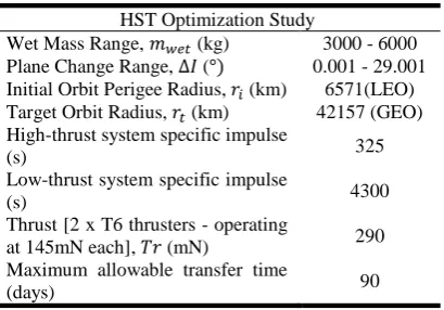
To demonstrate the capability of the optimization method described in this paper, a case study can be performed. The specification for this study is detailed in Table 1.

HST Optimization Study

Wet Mass Range, (kg) 3000 - 6000

Plane Change Range, ( ) 0.001 - 29.001 Initial Orbit Perigee Radius, (km) 6571(LEO) Target Orbit Radius, (km) 42157 (GEO) High-thrust system specific impulse

(s) 325

Low-thrust system specific impulse

(s) 4300

Thrust [2 x T6 thrusters - operating

at 145mN each], (mN) 290 Maximum allowable transfer time

(days) 90

Table 1 HST optimization study specification

A transfer from Low-Earth Orbit (LEO)/ Geostationary Transfer Orbit (GTO) to Geostationary Earth Orbit (GEO) is considered as this is a common transfer for large spacecraft. If the initial orbit is circular then the transfer is LEO-GEO and if the initial orbit is elliptical then the transfer is GEO. For the case of the GTO-GEO it is assumed the HST and bi-elliptic’s first high-thrust impulse is performed at the initial orbit perigee. The Hohmann transfer is performed as a one impulse manoeuvre at the initial orbit apogee. This impulse combines both the orbit raise and plane change. For the analysis, the high-thrust specific impulse is based on the 500N Bi-propellant European Apogee Motor1 and is a standard value amongst current technology[20]. The low-thrust system is based on the T6 thruster used in dual configuration [21,22]. A range of wet masses and plane changes are considered to give an overview of the HST performance. A selection of common GEO launch site latitudes are shown in Table 2 to relate the result to plausible launch scenarios.

Geostationary Earth Orbit Launch Site Latitudes Cape Canaveral, USA , ( ) 28.3 Kourou, French Giuana, ( ) 5.32 Sriharikota, India, ( ) 13.47

Xichang, China, ( ) 28.12

Table 2 Common geostationary earth orbit launch site latitudes[23]

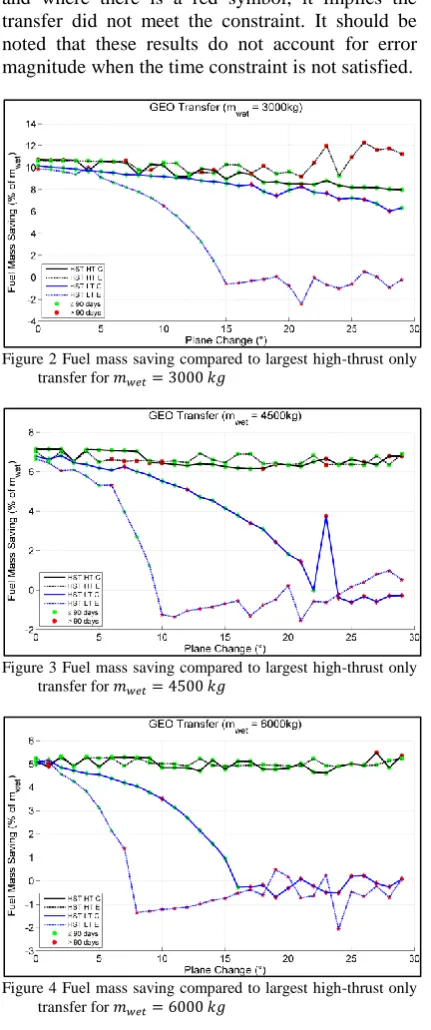
Figures 2 - 4 represent the fuel mass savings for the respective wet masses detailed in each figure title. The fuel mass saving is the difference between the HST dry mass and the largest dry mass delivered to

1

IAC-12-C1.6.7 Page 8 of 11 the target orbit by any of the high-thrust only

transfer comparisons. Each HST transfer is classified by the acronym detailed in the legend and defined at the beginning of the paper. Where there is a green symbol present, it infers the specified transfer has met the ninety day transfer constraint and where there is a red symbol, it implies the transfer did not meet the constraint. It should be noted that these results do not account for error magnitude when the time constraint is not satisfied.

Figure 2 Fuel mass saving compared to largest high-thrust only transfer for

Figure 3 Fuel mass saving compared to largest high-thrust only transfer for

Figure 4 Fuel mass saving compared to largest high-thrust only transfer for

From all three figures it is clear that the HST, utilizing a high-thrust plane change (circular or elliptical initial orbit), can deliver the largest fuel mass benefit and maintains a fairly constant fuel mass saving for all three wet masses considered. It can be seen that this is also true for the HST utilizing low-thrust plane change, starting in a

circular orbit, for a wet mass of . For the two remaining wet mass cases however it can be seen that there is a sharp decline in fuel mass saving with increasing plane change for both initial orbit cases considering the HST with low-thrust plane change. This would suggest that at smaller wet masses ( ), the HST with low-thrust plane change may be able to contend with the HST with high-thrust plane change. It is also evident with increasing plane change that the HST, utilizing low-thrust plane change, struggles to satisfy the transfer time constraint (identified by the increase in red markers). This is further accentuated with increasing wet mass and in some cases the high-thrust only transfer out-performs this version of the HST.

Table 3 gives a summary of the largest fuel mass savings for each wet mass case considered which satisfies the time constraint.

Max. Fuel Mass Savings Summary

Transfer _/ Saving (kg )

Plane Change ( ) HST HT C 320.07 / 10.67 3.001 HST HT E 317.99 / 9.09 0.001 HST HT C 321.6 / 8.04 2.001 HST HT C 321.6 / 7.15 1.001 HST HT C 320.73 / 6.41 1.001 HST HT C 320.57 / 5.83 0.001 HST HT C 319.83 / 5.33 2.001

Table 3 Largest fuel mass savings that meet the ninety day transfer constraint with specified transfer and plane change

It can be seen that the mass saving ( ) is fairly constant for all wet masses considered but the percentage saving of the wet mass ( ) is gradually decreasing with increasing wet mass. It is also found that the largest fuel mass savings occur at small plane change values and the HST with high-thrust plane change, starting in a circular orbit, offers the largest fuel mass saving for six out of seven case studies.

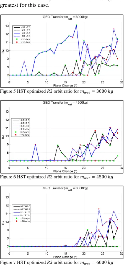
Figures 5-7 detail the orbit ratio for each transfer comparison. It can be seen a wet mass of

IAC-12-C1.6.7 Page 9 of 11 to the low-thrust system acceleration being the

greatest for this case.

Figure 5 HST optimized orbit ratio for

Figure 6 HST optimized orbit ratio for

Figure 7 HST optimized orbit ratio for

Figures 8-10 show the trends of the intermediate orbit eccentricity.

Figure 8 Intermediate orbit eccentricity for

Figure 9 Intermediate orbit eccentricity for

Figure 10 Intermediate orbit eccentricity for

It can be seen with increasing wet mass the maximum eccentricity in all HST variations reduces. It is also found that the general trend of the HST with high-thrust plane change (circular and elliptical initial orbit) is to increase intermediate orbit eccentricity with increasing plane change. Conversely, the HST with low-thrust plane change (circular and elliptical initial orbit) tends to decrease intermediate orbit eccentricity with increasing plane change.

VII.CONCLUSION

This paper has shown that substantial fuel mass savings are possible when utilizing the Hohmann Spiral Transfer (HST). For a transfer to Geostationary Earth Orbit it has been shown that a fuel mass saving of approximately

( ) is possible for a wet mass of – which satisfies a time constraint of . The HST with high-thrust plane change, starting in a circular initial orbit, offered the largest fuel mass saving for six out of seven case studies. With such a large fuel mass saving, it is thought a platform’s revenue could be improved by increasing the number of scientific payloads on-board.

IAC-12-C1.6.7 Page 10 of 11 HST with low-thrust plane change (circular or

elliptical initial orbit) may be able to compete with the HST high-thrust plane change.

The following trends have also been identified for the HST with high-thrust plane change (circular and elliptical initial orbit):

 As plane change increases

o the fuel mass saving stays fairly constant. o The intermediate orbit ratio tends to

increase.

o The intermediate orbit eccentricity tends to increase.

The following trends have also been identified for the HST with low-thrust plane change (circular and elliptical initial orbit):

 As plane change increases o the fuel mass saving reduces

o The intermediate orbit ratio tends to increase.

o The intermediate orbit eccentricity tends to decrease.

o The number of time constraint failures increases.

VIII. FUTURE WORK

Due to the sub-optimal nature of the high-thrust impulsive method, it is foreseen that future work will include the implementation of a method which optimizes each high-thrust impulsive burn in addition to the plane change distribution, , orbit ratio, , and intermediate orbit eccentricity, . As the methodology adopted for the HST high-thrust phase is the same used to determine the velocity requirement for the high-thrust only transfers (Hohmann and bi-elliptic), it is thought that the fuel mass saving will most probably stay the same. However, it is expected the overall dry mass delivered to the target will increase.

It is noted that this methodology, although adopted in this analysis for the HST, could be used to rapidly generate hybrid propulsion transfers of any nature. Future work will therefore consider different hybrid propulsion transfers and determine the feasibility of this methodology in comparison with other algorithms such as SEPSPOT[24]. A sensitivity study will also be performed to determine the error associated with the optimization process.

IX.REFERENCES

[1] S. Owens and M. Macdonald, “A Novel Method In Hybrid Propulsion Transfers,” in International Astronomical Congress, 2011, pp. 1–11.

[2] S. Owens and M. Macdonald, “An Extension and Numerical Analysis of the Hohmann Spiral Transfer,” in International Astronomical Congress, 2012.

[3] S. Owens and M. Macdonald, “Hohmann Spiral Transfer With Inclination Change Performed By Low-Thrust System,” in

23rd AIAA Spaceflight Mechanics Meeting, 2013.

[4] S. Owens and M. Macdonald, “Analogy to Bi-Elliptic Transfers Incorporating High- and Low-Thrust,” Journal of Guidance, Control, and Dynamics, vol. 36, no. 3, pp. 890–894, May 2013.

[5] A. E. Petropoulos, “Low-Thrust Orbit Transfers Using Candidate Lyapunov Functions with a mechanism for Coasting,”

AIAA.

[6] M. Macdonald and C. McInnes, “Analytical Control Laws for Planet-Centered Solar Sailing,” Journal of Guidance, Control, and Dynamics, vol. 28, no. 5, pp. 1038–1048, Sep. 2005.

[7] R. H. Battin, An Introduction to the Mathematics and Methods of

Astrodynamics, Revised Edition, Revised Ed. American Institution of Aeronautics and Astronautics, 1999, p. 799.

[8] A. Roy, Orbital motion, Fourth. IOP Publishing, 2005.

[9] M. J. H. Walker Ireland, B and Owens, J, “A Set of Modified Equinoctial Orbit Elements,” in in Celestial Mechanics 36, D. Reidel Publishing Company, 1985, pp. 409–419.

IAC-12-C1.6.7 Page 11 of 11 [11] C. Kluever, “Simple guidance scheme for

low-thrust orbit transfers,” Journal of Guidance Control and Dynamics, vol. 21, no. 6, pp. 19–21, 1998.

[12] J. Schoenmakers, J. Pulido, and R. Jehn, “SMART 1 Mission Analysis: Moon Option.”

[13] A. E. Petropoulos, “Simple Control Laws for Low-Thrust Orbit Transfers,” in

AAS/AIAA Astrodynamics Specialists Conference, 2003.

[14] D. A. Vallado, “Fundamentals of Astrodynamics and Applications,” in in

Fundamentals of Astrodynamics and Applications, 3rd ed., Microcosm Press and Springer, 2007, pp. 319–389.

[15] S. Owens and M. Macdonald, “A Complete Overview of the Hohmann Spiral

Transfer.” 2013.

[16] R. L. Burden and J. D. Faires, Numerical Analysis. Thomson Brooks/Cole Cengage Learning, 2011, pp. 48–56.

[17] S. Loney, Plane Trigonometry. Cambridge: University Press, 1893, pp. 173–183.

[18] J. Nocedal and S. J. Wright, Numerical Optimization. Springer, 2003, pp. 77–94.

[19] R. R. Bate, D. D. Mueller, and J. E. White,

Fundamentals of Astrodynamics. Dover Pubns, 1971, p. 198.

[20] M. Griffin and J. French, Space vehicle design Second Edition. 2004, p. 204.

[21] S. Clark, N. Wallace, Q. S. Division, and F. Guarducci, “Qualification of the T6 Ion Thruster for the BepiColombo Mission to the Planet Mercury,” in 32nd International Electric Propulsion Conference, 2011, pp. 1–23.

[22] J. S. Snyder, D. M. Goebel, R. R. Hofer, J. E. Polk, N. C. Wallace, and H. Simpson, “Performance Evaluation of the T6 Ion Engine,” Journal of Propulsion and Power, vol. 28, no. 2, pp. 371–379, Mar. 2012.

[23] W. Larson and J. Wertz, Space Mission Analysis and Design, Third. Microcosm

Press and K1uwer Academic PubUsbers, 1999, p. 733.