Coupled topology and pipe size optimization of water distribution systems

Coupled Topology and Pipe Size Optimization

of Water Distribution Systems

Salah H. A. Saleh1 and Tiku T. Tanyimboh2

Department of Civiland Environmental Engineering, University of Strathclyde Glasgow.

107 Rottenrow, Glasgow G4 0NG, UK

Salah H. A. Saleh, PhD Student

Department of Civil and Environmental Engineering, University of Strathclyde, Glasgow. 107 Rottenrow, Glasgow G4 0NG, UK.

Email: [email protected]

Tiku T. Tanyimboh, Senior Lecturer(Corresponding Author)

Department of Civil and Environmental Engineering, University of Strathclyde, Glasgow. 107 Rottenrow, Glasgow G4 0NG, UK.

Email: [email protected]; Tel: + 44 (0) 141 548 4366;

Fax: + 44 (0) 141 553 2066

This article was published in Water Resources Management (2013), 27(14): 4795-4814. DOI: 10.1007/s11269-013-0439-4.

Water Resources Management

November 2013, Volume 27, Issue 14, pp 4795-4814, DOI: 10.1007/s11269-013-0439-4

Coupled Topology and Pipe Size Optimization of Water Distribution Systems Salah H. A. Saleh, Tiku T. Tanyimboh

The final publication is available at www.springerlink.com;

Coupled Topology and Pipe Size Optimization of Water Distribution Systems

Salah H. A. Saleh and Tiku T. Tanyimboh

Department of Civil and Environmental Engineering, University of Strathclyde, Glasgow. 107 Rottenrow, Glasgow G4 0NG, UK

Abstract

This paper describes a new multi-objective evolutionary optimization approach to the simultaneous layout and pipe size design of water distribution systems. Pressure-deficient and topologically infeasible solutions are fully incorporated in the genetic algorithm without recourse to constraint violation penalties or tournaments. The proposed approach is demonstrated by solving three benchmark problems taken from the literature. New optimal layouts and/or new feasible solutions that are cheaper than the best solutions in the literature were found for both branched and looped network configurations. Specifically, a new best solution was generated for each of the above-mentioned benchmark problems. In addition, the case of the looped design of a hitherto branched network in the literature was considered. Detailed results are included that show that the proposed approach achieves good solutions efficiently and consistently.

Key words: water distribution system, topology optimization, penalty-free evolutionary approach, multi-objective optimization, genetic algorithm, EPANET 2

1. Introduction

Water distribution systems (WDSs) are a vital part of the infrastructure in developed societies. However, WDSs deteriorate with time and require periodic maintenance to maintain the system capacity at the required levels. This increases considerably the overall cost of the system. Even though the capital cost is made up of the costs of system components such as pipes, valves, tanks and pumps, the capital cost is mainly due to pipeline provision and construction (Djebedjian et al 2008). The operation cost is mainly due to energy and water treatment costs. Constructing and putting WDSs into operation is very expensive and it follows that good planning of the layout of the network of pipes can lead to a substantial reduction in the capital cost in addition to the long-term maintenance and operation costs.

cost is relatively low, they are easy to operate and are suitable for sparsely populated areas (Swamee and Sharma 2008). Branched systems have only one supply path from the source to any demand point (Swamee and Sharma 2008). This has the disadvantage of cutting off the water supply to the consumers downstream of any section of pipe that is not in service, e.g. due to a mains break. To reduce the effect of such situations, looped systems that have multiple supply paths from the source to the demand points are preferred. The reliability and cost of looped systems is highly dependent on the number of loops (Tanyimboh and Sheahan 2002; Tanyimboh and Setiadi 2008).

Most of the current investigations on WDS optimization have focused on designing a fixed layout. However, there are some situations in which designing a predefined layout is rarely optimal in real systems. For example, designing new systems or expanding existing systems where in general it will be impossible to determine the best configuration a priori. Determining the best layout is not only important for new systems. Expanding existing systems due to rehabilitation or upgrading purposes represents an opportunity to improve existing layouts, for example. Also, optimizing the layout of branched WDSs can achieve significant cost savings (Afshar 2007a). Despite the obvious benefits, joint layout and pipe size optimization has received little attention, probably because of the extra complexity involved (Morgan and Goulter 1985; Afshar 2007a) which in part is attributable to the strong coupling between the layout and pipe sizes.

infeasible solutions from the optimization process. Moreover, the fact that penalty functions incorporate factors that are problem-specific made the previous studies time-consuming. Layout and pipe size optimization in such approaches is preceded by a trial and error procedure to design a penalty function that is valid only for the network under consideration. This has the disadvantage of being laborious when employing such approaches to design new WDSs. In addition, there is no guarantee that the designed penalty function is optimal.

This paper describes a new penalty-free multi-objective evolutionary approach to the simultaneous layout and pipe size optimization of WDSs. We adopted an approach in which the entire solution space that consists of both feasible and infeasible solutions is exploited in full. In particular, infeasible solutions are not targeted and removed arbitrarily purely by virtue of their infeasibility or by the use of extraneous penalties. The effectiveness of the approach is demonstrated by solving three benchmark problems. Better solutions than the best solutions in the literature were found for all the above-mentioned benchmark problems. By optimizing the layout and pipe sizes simultaneously and assessing infeasible solutions rationally, new least cost designs and/or new optimal layouts were found. In addition, a hitherto branched design optimization problem in the literature was solved as a looped design.

2. LITERATURE REVIEW

(1982) developed an approach that contained two linear programs, one for determining the optimum layout and the other for pipe sizing. However, there was no guarantee that the designs generated would be fully looped as the criterion used was a simple requirement to connect each node using two pipes as opposed to two independent paths. Kessler et al. (1990) and Cembrowicz (1992) tackled the problem by choosing links for either addition or removal from a predefined base graph. The base graph is the network consisting of the full set of feasible links. All the above-mentioned approaches were based on an assumption that the problem could be divided into two separate optimization problems in which layout optimization is followed by pipe size optimization. However, the relationship between the layout and the pipe diameters is strong and sequential procedures as described above can be expected to yield suboptimal results.

Also, Afshar et al. (2005a) developed an iterative two-stage approach such that, in the first stage, the optimal diameters for a predefined layout are determined using a non-linear programming method. In the second stage, an iterative pipe removal search process is carried out to reduce the cost without undermining the node connectivity constraint. Any infeasible solutions generated in the early stages due to the randomness in creating the initial population of solutions by the GA are gradually discarded using constraint violation penalties. To ensure the feasibility of branched solutions, at least one independent path from the source nodes to each of the demand nodes is required. Afshar (2005b and 2007a,b) also proposed several approaches that basically restricted the evolutionary algorithms used to feasible solutions. These included a genetic algorithm using three modified roulette wheel selection schemes (Afshar 2007a), the conventional roulette wheel (Afshar 2007b) and a max-min ant algorithm (Afshar 2005b).

3. MAIN HYDRAULIC EQUATIONS

The performance of WDSs is governed by the following system of nonlinear equations. ( ) ( ) ,...,N j Q Q Q _j N out ij ij N in ij ij j j 1 = = −

∑

∑

ij = ∀

∑

0 (2)

h_ij =α L_ij

(

)

where N = number of nodes; l represents the set of pipes in the closed circuit of pipes that form a loop; Qj = demand or supply at node j;in(Nj) and out(Nj) = all

pipe flows to and from node j, respectively; α = dimensionless conversion factor (10.6844 in SI units); Cij, Dij, hij, Lij and Qij = Hazen-Williams roughness

coefficient, diameter, headloss, length and flow rate respectively for pipe ij; H_j

and des j

H = actual and desired head respectively at node j. The desired head is the head at a node above which demands are satisfied in full. Equation (1) is for conservation of mass while Equation (2) is for conservation of energy; and Equation (3) is the Hazen-Williams pipe friction headloss formula. Equation (4) ensures there is sufficient pressure at each demand node. In the UK, for example,

Hjdes is often taken as a minimum residual pressure head of 15m (Ofwat 2008).

Equations (1) to (3) are usually handled by employing a hydraulic simulator -- e.g. EPANET 2 (Rossman 2000), EPANET-MSX (Shang et al. 2008), PRAAWDS (Tanyimboh and Templeman 2010), EPANET-PDX (Siew and Tanyimboh 2012), etc. -- which ensures these equations are automatically satisfied. Various approaches have been used in the literature to address Equation (4) in the design process. We developed a novel unified feasibility measure that accounts for both nodal pressures and network topology. This is explained in detail in the following section.

4. PROBLEM FORMULATION

assumptions. (1) The network configuration including all of the feasible links is known. This network is termed the fully connected network herein. (2) The pipe diameters and the links to be included or excluded are the decision variables of the problem. The aim is to find and size the optimal subset of links. (3) Water demands are located at the nodes. In reality, demands occur along the pipes but for ease of analysis, they are aggregated and allocated at the nodes. (4) Node demands are known with certainty. Although nodal demands may be uncertain in practice, demands and other WDS aspects that can lead to uncertainty are not addressed herein. (5) The required pressure head at each demand node is given. (6) Finally, design is to be optimized based on the initial construction cost only. Even though the operational and other whole-life costs (Tanyimboh and Kalungi 2008) contribute significantly to the whole cost of the system, their inclusion is beyond this study.

If cij denotes the cost per unit length for pipe ij, the cost objective function can be

written as

∑

ij ij ij

1 c L

f Cost (5)

(

)

∑

RHD (6)

in which RHD is the residual head deficit for the entire network. In the case of a node having Hj≥Hdesj , it is assigned a deficit of zero. In other words, the residual head deficit RHD will be zero only if a design is feasible.

Secondly, to optimize the layout and pipe sizes simultaneously a pipe diameter of zero was introduced to enable different layouts to be generated by removing any link from the fully connected network (Afshar 2007b). A diameter of zero in Equation (5) yields zero cost, which reflects the real situation for a non-existent link. However, this results in an undefined value of the headloss in Equation (3). Therefore, to resolve this problem, the link removal case was modelled as a closed pipe when simulating the WDS. Since link removal takes place randomly especially in the early phases of the optimization, some nodes or even parts of the network can become disconnected from the source nodes. To avoid this, Equation (6) was extended to account for layout infeasibility. For a branched layout to be feasible, a minimum of one supply path is required for each demand node. For looped networks, at least two independent supply paths per demand node are required. The extent of layout infeasibility was quantified as the sum of the individual nodal shortfalls in the required number of independent supply paths. Accordingly, Equation (6) was augmented as follows.

(

)

(

)

[

]

ity Infeasibil Total f j des j j j j des j 2 < ∀ < ∀ − + − = =

where NPj is the number of independent supply paths for node j while R is the

minimum number of independent paths required. For a node with NPj ≥ R, the

second term in Equation (7) is assigned a value of zero. R = 1 for branched networks and R = 2 for looped networks. The total infeasibility in Eq. 7 is equal to zero if and only if a design is both topologically and hydraulically feasible.

Due to the large difference in the respective ranges of the objective function values in Equations (5) and (7), each objective was normalized to maintain the objectives within the interval [0, 1], i.e.

min , max ,

min , ,

i i

i j i

f f

f f

− −

(8)

in which fi,min and fi,max are the respective minimum and maximum values of the

ith objective function and fi,j is the value of the ith objective function for the jth

candidate solution in the current population.

5. COMPUTATIONAL SOLUTION

It is worth observing that EPANET 2 often produces unrealistic results of node pressures and pipe flows within parts of the network that are not connected to a source. For example, isolated nodes are assigned arbitrarily large negative pressures while pipes having an isolated upstream node are dealt with as if they are connected to the source. We resolved this problem by developing an algorithm for detection of both isolated nodes and pipes that assigns zero flow and pressure, respectively, to any pipes and nodes that are not connected to a source. By addressing the problem of disconnected network components we were able to assess the fitness of both feasible and infeasible solutions in a consistent and bias-free manner.

6. BENCHMARK EXAMPLES

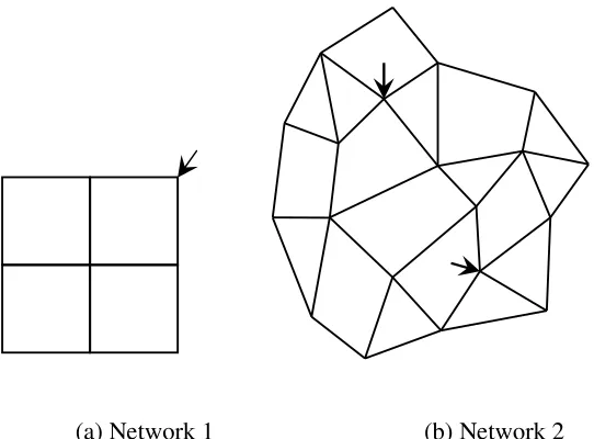
The two benchmark networks (Figure 2) considered are described briefly in turn in this section ahead of the results in Section 7. Both branched and fully-looped designs were considered for each of the two networks. A bit-wise mutation operator was used and mutation rates in the range 0.001 to 0.3 were investigated. This sensitivity analysis would appear to suggest that the optimum mutation rate is pm≈ 1/ng where pm = mutation rate and ng = chromosome length as determined

by the number of genes. A Core 2 Duo desktop computer that has a processor speed of 2.99GHz and 3GB of RAM was used.

Network 2 (Figure 2) is part of the Winnipeg system (Morgan and Goulter 1985). This network has 2 sources, 20 nodes and 37 pipes. The Hazen-Williams roughness coefficient for all pipes is 130. Allowing for pipe removal, the solution space of this network comprises a combined total of 1437 = 2.55×1042 hydraulically and/or topologically feasible and infeasible solutions. Using a 4-bit binary substring, since this network has 37 pipes, each solution was represented with a chromosome whose length is 148 genes. The resulting redundant codes from this representation were mapped to the link removal option. A uniform crossover operator was used to create two offspring from two parents using a crossover probability of 1. Bit-wise mutation was used to flip the selected bit either from 0 to 1 or from 1 to 0 using a mutation probability of 1/ng = 1/148.

7. RESULTS AND DISCUSSION

The results for the four design problems are discussed below in turn. We have included indicative statistics for the consistency and quality of the solutions. In the results tables that follow, the relative frequencies of the various solutions found in multiple runs of the GA are displayed graphically in terms of the deviations of the respective costs from the cost of the best known solution. Given any number of random GA runs and their respective least cost solutions, the relative cost deviation of each solution is defined here as the ratio of the deviation of the cost to the maximum cost deviation among the solutions under consideration.

7.1 BRANCHED DESIGN OF NETWORK 1

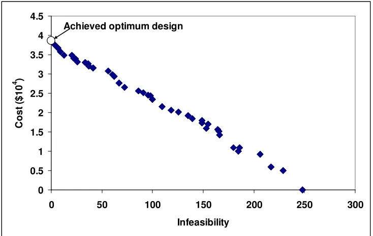
at the critical node would appear to suggest that the achieved solution is at least a near-global optimum. Figure 4 shows the best achieved Pareto Optimal Front (POF) for Network 1. With reference to Equation (7), the maximum infeasibility value of f2 = 248 (Figure 4) is the summation of the prescribed minimum nodal

residual pressure head of 30 m and the minimum required nodal connectivity of R = 1, for all the eight demand nodes, i.e. (30 + 1) × 8 = 248. With a cost of zero this solution is always non-dominated. This zero cost solution has no pipes. Consequently, selecting the zero cost solution for crossover results in link removal in the offspring. This zero cost solution is very important as it safeguards the potential for creating new layouts in every generation.

Table 2 summaries the results to date and demonstrates clearly the effectiveness of the proposed approach. The best design generated costs $38,600 and is actually the cheapest solution to date. The GA was run 10 times using different randomly created initial populations. A maximum of 200,000 function evaluations were allowed for each GA run. Using a population of 100, the optimum design having a cost of $38,600 was identified in 8 different runs out of 10. The best run took a CPU time of about 10 seconds after 10,400 function evaluations. The two remaining runs both found a feasible solution that costs $39,800. The average, median and maximum value of the least cost for the 10 GA runs were $38,840, $38,600 and $39,800 respectively. The standard deviation (SD), coefficient of variation (CV) and SD/f1* were $505.96, 0.0130 and 0.0131, respectively. f1* =

$38,600 is the cost of the optimal solution. It can be seen that the values of CV

and SD/f1* are small and similar. CV is indicative of the consistency of the results

whereas SD/f1* is indicative of the quality of the results; self-evidently the smaller

were also found by the 10 GA runs as shown in Table 2.

7.2 LOOPED DESIGN OF NETWORK 1

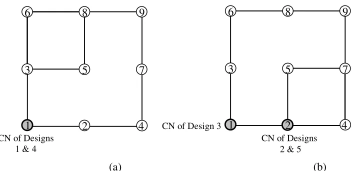
Network 1 was also optimized as a looped network. Two different optimal layouts each with an associated optimal design (Designs 1 and 2) were created (Figure 5 and Table 3). Figure 6 shows the best POF achieved. As all hydraulically and topologically feasible designs have an infeasibility value of zero the non-domination sorting procedure ensures that only the cheapest feasible design can survive at the feasibility boundary as the least cost looped design. There are a few hydraulically feasible branched designs next to the least cost looped design (Figure 6). The maximum infeasibility value of 258 is the sum of the nodal head deficit for all nodes with insufficient pressure and supply paths shortfall for all nodes with less than two independent supply paths. Since all of the 8 demand nodes in this design are not connected to the source node the first term of Equation (7) results in a residual head deficit of 8 × 30 = 240 m. In addition, all 9 network nodes contribute a further infeasibility value of 9 × 2 = 18 through the second term in Equation (7). Inherently, infeasible solutions dominate the POF (Figure 6); all feasible solutions except for the cheapest are dominated as explained above.

Using a population of 100, the GA was run 20 times due to the increased problem complexity and larger solution space using different randomly created initial populations. The complexity arises from the existence of alternative feasible flow distributions for looped networks. A maximum of 200,000 function evaluations per GA run were allowed. Interestingly, two different optimum designs having a

were achieved after 5,000 and 10,500 function evaluations respectively. The CPU time was about 4.8s and 10.1s for Designs 1 and 2 respectively. Designs 1, 2 and 3 in Table 3 were identified 5, 3, and 10 times respectively by the 20 random GA runs. Each of Designs 4 and 5 in Table 3 was found once. The average, median and maximum value of the least cost were $41,885, $42,200 and $42,300 respectively. The SD, CV and SD/f1* values were $406.88.96, 0.0097 and 0.0098,

respectively. It is worth highlighting that the least cost branched design of this network having a cost of $38,600 was identified 13 times by the 20 GA runs. This result is significant in that it suggests it may be possible to combine and solve the branched and looped least cost network design problems together.

7.3 BRANCHED DESIGN OF NETWORK 2

Tables 4 and 5 and Figure 7 show the results for the branched design of Network 2. The solution of $1,684,228 (Design 1) is the cheapest design to date while the near-optimal solution of $1,692,058 (Design 2) is also cheaper than the best solution in the literature. The layout of Design 1 has not been identified previously. Its creation here is, therefore, a remarkable achievement. Two single-source branched networks were created by removing 19 pipes (51%) out of 37 in each of Designs 1 and 2. 20 GA runs were performed using different randomly created initial populations. The termination criterion was 500,000 function evaluations. The least cost of f1* = $1,684,228 (Design 1) was identified two times

out of 20. Using a population of 100, this required 154,500 function evaluations and a CPU time of about 2.12 minutes according to the best POF. Design 2 was identified once among the 20 runs. The average, median and maximum values of the least cost were $1,753,359, $1,733,044 and $1,889,386 respectively. The SD,

shows the best achieved POF. A good distribution of solutions is evident. This may be attributable to the larger solution space made up of a large number of branched layouts and pipe size combinations.

7.4 LOOPED DESIGN OF NETWORK 2

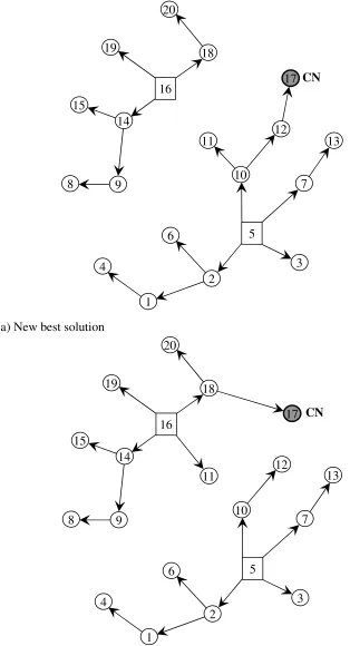
Tables 6 to 8 and Figure 9 show the results for the looped design of Network 2. Remarkably, three new feasible solutions that are cheaper than the previous best solution in the literature were created. A new layout was created also, as shown in Figure 9b. The new layout is that of the new cheapest solution of f1* = $1,972,559

(Design 3) that has only 25 pipes. The previous best solution has 26 pipes (Figure 9a). 20 random runs of the GA using different starting points were performed. Using a population of 100, the cheapest design of $1,972,559 was identified two times out of 20 the best of which took 901,300 function evaluations. This took a CPU time of about 12.41 minutes. Two of the 20 runs resulted in Near-optimal Designs 1 and 2 respectively. The termination criterion was 1,000,000 function evaluations. The average, median and maximum values of the least cost were $2,019,891, $1,998,076 and $2,095,167 respectively. The SD, CV and SD/f1*

values were $43,683.82, 0.0216 and 0.0222.

has zero infeasibility. The cheapest feasible branched solution among the 20 conducted GA runs has a cost of $1,694,966, which is slightly more expensive than the cheapest branched design of $1,684,228 (Tables 4 and 5).

8 CONCLUSIONS

This article provides strong evidence to support the incorporation of infeasible solutions in the design optimization of water distribution networks. Arbitrarily penalizing or removing hydraulically or topologically infeasible solutions can lead to the loss of some essential features of the optimal solution from the gene pool. By contrast, the penalty-free fully inclusive approach developed does not avoid infeasible solutions and retains the advantage of progressing towards the optimum solution from both the feasible and infeasible sections of the solution space. It is believed the performance of the algorithm is enhanced in this way by virtue of the presence of both feasible and infeasible non-dominated near-optimal solutions in successive generations. For problems involving layout optimization, a procedure for handling topologically infeasible solutions in a rational manner is a precondition if the entire solution space is to be exploited in full. We addressed this issue in this article.

the least cost feasible solution. Besides cost, a possible remedy might include the introduction of additional hydraulic performance objectives in order to differentiate the feasible solutions further. In addition, design should be based on minimizing the whole-life costs rather than the initial construction cost only. It is recognised also that the infeasibility measure adopted is dimensionally inconsistent. Further improvements are thus indicated.

REFERENCES

Afshar, M.H., Akbari, M., and Marino, M.A. (2005a) Simultaneous layout and size optimization of water distribution networks: engineering approach. J. Infrastruct. Syst., 11(4), 221-230.

Afshar, M.H. (2005b) Application of max-min ant system for joint layout and size optimization of pipe networks. Proceedings of 9th international water technology conference. IWTC9, 17-20 March, Sharm El-Sheikh, Egypt, 593-608.

Afshar, M.H. and Jabbari, Ibrahim (2007a) Simultaneous layout and size optimization of pipe networks using genetic algorithms. Arabian J. Sci. and Eng., 33(2B), 391-409.

Afshar, M.H. (2007b) Evaluation of selection algorithms for Simultaneous layout and size optimization of water distribution networks. Scientia Iranica, 14(1), 23-32.

Cembrowicz, R.G. (1992) Water Supply Systems Optimization for Developing Countries. In: B. Coulbeck and E. Evans, eds. Pipeline Systems (Fluid Mechanics and its Applications). Kluwer Academic, London, UK, 59-76.

Davidson, J.W. and Goulter, I.C. (1995) Evolution Program for Design of Rectilinear Branched Networks. J. Comp. in Civ. Eng., 9(2), 112-121.

Deb, K., Pratap, A., Agarwal, S. and Meyarivan, T. (2002) A Fast and Elitist Multiobjective Genetic Algorithm: NSGA-II. IEEE Trans. on Evo. Comp., 6(2), 182-197.

Djebedjian, B., Yaseen, A. and Ezzeldin. R. (2008)Reliability-Based Optimization of Layout and Sizing of Water Distribution Systems. Proceedings of the 12th International Water Technology Conference. IWTC12, 27-30 March, Alexandria. Egypt, 759-779.

Geem, Z.W., Kim, J.H., and Yoon, Y.N. (2000) Optimal Layout of Pipe Networks Using Harmony Search. Proceedings of 4th International Conference on Hydro-Science and Engineering. 26-29 September, Seoul, South Korea.

Goldberg, D. E. (1989) Genetic algorithms in search, optimization and machine learning. 1st ed. USA: Addison-Wesley Longman Publishing Co.

Kessler, A., Ormsbee, L., and Shamir, U. (1990) A Methodology for Least-Cost Design of Invulnerable Water Distribution Networks. Civ. Eng. Syst., 7(1), 20-28.

Morgan, D.R. and Goulter, I.C. (1982) Least cost layout and design of looped water distribution systems. Proceedings of 9th International Symposium on Urban Hydrology, Hydraulics and Sediment control. University of Kentucky, Lexington, KY, USA, 27-30.

Ofwat (2008) Guaranteed Standard Schemes [online]. Ofwat. Available from: http://www.ofwat.gov.uk/consumerissues/rightsresponsibilities/waterpressure [Accessed 29 January 2012].

Rossman, L.A. (2000) EPANET 2: Users Manual. Cincinnati, USA: U.S. Environmental Protection Agency.

Rowel, W.F. and Barnes, J.W. (1982) Obtaining the Layout of Water Distribution Systems. J. Hydraulics Division, 108(1), 137-148.

Shang, F. Uber, J.G. and Rossman, L.A. (2008) Modelling reaction and transport of multiple species in water distribution systems. Env. Sc. and Tech. 42(3), 808-814.

Siew, C. and Tanyimboh, T.T. (2012) Pressure-dependent EPANET extension. Water Resources Management, 26(6), 1477-1498.

Swamee, Prabhata K. and Sharma, Ashock K. (2008) Design of Water Supply Pipe Networks. New Jersey: John Wiley & Sons.

Tanyimboh, T.T. and Kalungi, P. (2008) Optimal long-term design, rehabilitation and upgrading of water distribution networks. Engineering Optimization, 40(7), 637-654.

Tanyimboh, T.T. and Sheahan, C. (2002) A maximum entropy based approach to the layout optimization of water distribution systems. Civ. Eng. and Environ. Syst., 19(3), 223-253.

Tanyimboh, T.T. and Setiadi, Y. (2008) Joint layout, pipe size and hydraulic reliability optimization of water distribution systems. Eng. Optim., 40(8), 729-747.

Tanyimboh, T.T. and Templeman, A.B. (2010) Seamless pressure-deficient water distribution system model. J Water Manag, 163(8), 389-396.

Walters, G.A. and Lohbeck, T.K. (1993) Optimal Layout of Tree Networks Using Genetic Algorithms. Eng. Optim., 22(1), 27-48.

Figure 1: Diagrammatic overview of proposed approach

NSGA-II Loop

No

Yes Start

Define fully connected network

Initial random population

EPANET 2 hydraulic simulation of generated designs

Does the design have isolated node(s) and link(s)

Algorithm for automatic detection of isolated nodes

Evaluate design cost and infeasibility

Non-dominated sorting of generated designs

Cross-over and mutation to generate new population

Stopping criterion satisfied Stop No

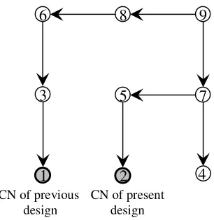
Figure 3: Optimal branched layout for Network 1 (CN denotes Critical Node) 2

1 6

5 7

4 9 8

3

CN of previous design

0 0.5 1 1.5 2 2.5 3 3.5 4 4.5

0 50 100 150 200 250 300

Infeasibility

C

o

s

t

($

1

0

4 )

Achieved optimum design

(a) (b) Figure 5: Optimal looped layouts for Network 1 (CN denotes Critical Node)

6

5 7

4 9 8

3

2 1

CN of Designs 2 & 5 CN of Design 3

1 6

5 7

4 9 8

3

2

0 0.5 1 1.5 2 2.5 3 3.5 4 4.5

0 50 100 150 200 250 300

Infeasibility

C

o

s

t

($

1

0

4 )

Best solution

Hydraulically feasible branched solutions Infeasible solutions

(a) New best solution

(b) Previous best solution (Afshar et al. 2005)

Figure 7: Optimal branched layouts for Network 2 (CN denotes Critical Node) 20

8 9

18 19

14 15

16

3 7

2 4

6

13 12

10 11

5

1

CN 17

20

8 9

11 18 19

14 15

16

CN 17

3 7

2 4

6

12

10

5

1

0 0.2 0.4 0.6 0.8 1 1.2 1.4 1.6 1.8

0 200 400 600 800 1000 1200 1400

Infeasibility

C

o

s

t

($

1

0

6 )

Achieved Optimum design

(a)

(b)

Figure 9: Optimal looped layouts for Network 2 (CN denotes Critical Node) 3

20

7

2 6

8 9

17 12 10 11 18 19 14 15 16 5 1 4 CN of design 3 13 3 20 7 2 4

8 9

17 10 11 18 19 14 15 16 5 1

13 _{design 1} CN of 12

CN of design 2

CN of the previous design

0 0.5 1 1.5 2 2.5

0 200 400 600 800 1000 1200 1400

Infeasibility

C

o

s

t

(£

1

0

6 )

Best solution

Hydraulically feasible branched solutions Infeasible solutions

0 0.5 1 1.5 2 2.5

0 200 400 600 800 1000 1200 1400

Infeasibility

C

o

s

t

($

1

0

6 )

Run 1 Run 2

Run 3 Run 4

Run 5 Run 6

Run 7 Run 8

Run 9 Run 10

Run 11 Run 12

Run 13 Run 14

Run 15 Run 16

Run 17 Run 18

Run 19 Run 20

Table 1: New and previous cheapest feasible branched designs for Network 1

Pipe

Diameter (mm)

Node

Head (m) Surplus head (m) Afshar

(2007a) Present

Afshar

(2007a) Present

Afshar

(2007a) Present

1-3 100 100 1 30.21a 30.21 0.21a 0.21a

2-5 120 100 2 30.94 30.06a 0.94 0.06

3-6 120 120 3 32.12 32.12 0.12 0.12

4-7 100 100 4 32.89 32.90 0.89 0.90

5-7 120 140 5 33.78 36.94 0.78 0.94

6-8 140 140 6 34.95 34.95 0.95 0.95

7-9 140 140 7 39.78 39.77 0.78 0.77

8-9 140 140 8 39.78 39.77 0.78 0.77

0 0 0.2 0.4 0.6 0.8 1 0 0.2 0.4 0.6 0.8

Relative Cost Deviation

R e la ti v e F re q u e n c y

0 0.2 0.4 0.6 0.8 1

0 0.2 0.4 0.6 0.8 1

Relative Cost Deviation

R e la ti v e F re q u e n c y

Table 2: Summary of the cheapest feasible branched and looped designs for Network 1

a_{A direct comparison is not possible as a hybrid approach involving a tree growing algorithm and} harmony search was used. bNew best least-cost feasible solution

Design Case Author Approach Cost ($) Function

evaluations

Branched

Geem et al (2000)

Layout optimization followed by pipe

sizing using harmony search 39,800 N/A a

Afshar (2005b) Simultaneous layout and pipe size

optimization using max-min ant system 39,800 7,900

Afshar (2007a)

Simultaneous layout and pipe size optimization using GA with four

crossover selection schemes

39,400 7,500

Afshar (2007b)

Simultaneous layout and pipe size optimization using GA with three

crossover selection schemes

39,400 7,500

10 random runs of the proposed

approach

39,800 9,500

39,700 9,900

39,600 21,100

39,400 28,200

38,600b _10,400

Looped

20 random runs of the proposed

approach

42,300 198,100

42,200 112,100

42,200 7,200

41,400 10,500

Table 3: Results of the optimum looped designs achieved for Network 1

Pipe Diameter (mm) Node Head (m)

Des. 1 Des. 2 Des. 3 Des. 4 Des. 5 Des.1 Des.2 Des.3 Des.4 Des.5 1-2 100 80 80 100 80 1 30.04a _30.13a _{30.07 30.07}a _30.03a 1-3 80 100 100 80 80 2 31.26 30.66 30.06a 30.67 31.00 2-4 140 100 80 120 80 3 30.37 31.18 32.02 31.41 32.33 2-5 - 80 100 - 100 4 33.72 35.00 30.76 35.08 33.69

3-5 100 - - 80 - 5 32.25 33.70 34.99 33.67 36.17

3-6 80 100 120 100 100 6 30.72 36.40 34.88 32.82 36.96 4-7 140 140 100 140 120 7 40.44 38.88 39.81 41.18 38.52 5-7 - 100 120 - 140 8 39.08 40.63 39.73 38.27 40.95

5-8 100 - - 100 -

6-8 100 140 140 120 140

7-9 140 140 140 140 140

8-9 140 140 140 140 140

Table 4: New and previous optimum branched designs for Network 2

Pipe

Diameter (mm)

Node

Head (m) Surplus head (m)

Afshar (2005a) Present approach Afshar (2005a) Present approach Afshar (2005a) Present approach Des. 1 (Fig. 10) Des. 2

(Fig. 11) Des. 1 Des. 2

Des. 1

Des. 2

1-2 400 400 400 1 83.68 79.37 83.69 8.68 4.37 8.69

1-4 300 350 300 2 94.67 90.34 94.67 20.67 16.34 20.67

2-5 550 500 500 3 80.85 80.85 80.86 7.85 7.85 7.86

2-6 250 300 250 4 75.23 75.38 75.25 3.23 3.38 3.25

3-5 250 250 250 5 102.00 102.00 102.00 - -

5-7 350 350 400 6 74.85 82.20 74.86 1.85 9.20 1.86

5-10 350 450 350 7 72.28 72.31 86.50 5.28 5.31 19.5

7-13 350 350 300 8 76.04 73.03 73.03 4.04 1.03 1.03

8-9 350 350 350 9 80.36 77.35 77.35 10.36 7.35 7.35

9-14 400 400 400 10 82.37 80.27 82.38 13.37 11.27 13.38

10-11 - 300 - 11 82.42 74.26 82.43 11.42 3.26 11.43

10-12 300 400 300 12 72.85 71.56 72.87 2.85 1.56 2.87

11-16 300 - 300 13 65.51 65.53 72.15 1.51 1.53 8.15

12-17 - 350 - 14 90.88 87.85 87.85 17.88 14.85 14.85

14-15 250 300 300 15 74.32 81.05 81.05 1.32 8.05 8.05

14-16 550 500 500 16 96.00 96.00 96.00 - -

16-18 400 350 400 17b 67.15 67.34 67.17 0.15 0.34 0.17 16-19 300 300 300 18 80.97 83.07 80.98 10.97 13.07 10.98 17-18 300 - 300 19 81.93 81.93 81.93 11.93 11.93 11.93

18-20 300 300 300 20 68.78 70.89 68.79 1.78 3.89 1.79

Cost ($) 1,693,393 1,684,228a _1,692,058a

0 0 0.2 0.4 0.6 0.8 1 0 0.05 0.1 0.15 0.2

Relative Cost Deviation

R e la ti v e F re q u e n c y

Table 5: Summary of the new and previous optimal branched designs for Network 2

a_{Two new best least cost feasible solutions.} b _{A direct comparison is not possible as two} sequential stages incorporating an iterative search procedure were used.

Author Approach Cost ($) Function

evaluations

Afshar (2007b)

Simultaneous layout and pipe size optimization using GA with four crossover selection schemes

1,783,086 100,000

Afshar (2007a)

Simultaneous layout and pipe size optimization using GA with three crossover selection schemes

1,783,086 100,000

Afshar (2005b) Simultaneous layout and pipe size

optimization using max-min ant system 1,710,121 22,800

Afshar (2005a)

Iterative two-stage procedure with sequential layout and pipe size

optimization 1,693,393 N/A

b

20 random runs of the proposed approach

1,692,058a 170,300

Table 6: New and previous optimal looped designs for Network 2

Pipe

Diameter (mm)

Afshar (2005a)

Present approach

Design 1a _{Design 2}a _{Design 3}a

1-2 400 400 400 400

1-4 350 300 300 300

2-5 500 500 500 500

2-6 250 250 250 250

3-5 250 250 250 250

3-7 125 200 125 125

4-8 125 125 125 125

5-7 350 350 350 400

5-10 350 400 350 350

6-9 125 125 125 -

6-10 - - - 150

7-13 300 300 300 300

8-9 350 400 350 350

8-15 - - - -

9-14 400 400 400 400

10-11 150 250 150 -

10-12 300 300 300 250

11-12 - - - 200

11-16 250 150 250 300

12-17 125 150 125 -

13-17 125 150 150 125

14-15 350 250 250 250

14-16 500 500 150 500

15-19 150 125 125 125

16-18 450 400 450 400

16-19 250 300 300 300

17-18 300 300 300 300

18-20 300 300 250 300

19-20 125 150 200 125

Table 7: Nodal heads of the new and previous optimal looped designs of Network 2

Node

Head (m) Surplus head (m)

Afshar (2005a)

Present approach _Afshar

(2005a) Present approach

Des. 1 Des. 2 Des. 3 Des. 1 Des. 2 Des. 3

1 79.07 80.14 80.27 80.30 4.07 5.14 5.27 5.30

2 90.44 90.79 90.88 91.08 16.44 16.79 16.88 17.08

3 78.56 77.25 78.95 82.69 5.56 4.25 5.95 9.69

4 74.80 72.20 72.38 72.16 2.80 0.20 0.38 0.16a

5 102.00 102.00 102.00 102.00 - - - -

6 73.02 73.23 73.97 76.34 0.02a 0.23 0.97 3.34

7 74.65 76.34 76.12 85.51 7.65 9.34 9.12 18.51

8 72.52 73.99 74.50 72.85 0.52 1.99 2.50 0.85

9 76.58 76.37 79.10 77.32 6.58 6.37 9.10 7.32

10 79.46 81.44 79.33 84.42 10.46 12.44 10.33 15.42

11 72.72 72.19 72.68 76.10 1.72 1.19 1.68 5.10

12 70.40 70.38 70.15 70.65 0.40 0.38 0.15a 0.65

13 68.37 64.00 64.34 70.40 4.37 0.00a 0.34 6.40

14 87.29 87.76 90.69 88.02 14.29 14.76 17.69 15.02

15 78.57 73.23 74.96 73.57 5.57 0.23 1.96 0.57

16 96.00 96.00 96.00 96.00 - - - -

17 71.15 67.83 70.53 68.96 4.15 0.83 3.53 1.96

18 86.90 81.84 87.98 81.94 16.90 11.84 17.98 11.94

19 70.79 78.01 75.83 78.73 0.79 8.01 5.83 8.73

20 73.77 71.78 69.14 71.22 6.77 4.78 2.14 4.22

0 0.2 0.4 0.6 0.8 1 0 0.05 0.1 0.15 0.2

Relative Cost Deviation

R e la ti v e F re q u e n c y

Table 8: Summary of the new and previous least cost feasible looped designs of Network 2

Author Approach Cost ($) Function

evaluations

Afshar (2007b)

Simultaneous layout and pipe size optimization using GA with four crossover selection schemes

2,056,379 100,000

Afshar (2007a)

Simultaneous layout and pipe size optimization using GA with three crossover selection schemes

2,056,379 100,000

Afshar (2005b) Simultaneous layout and pipe size

optimization using max-min ant system 2,055,917 31,500

Afshar (2005a)

Iterative two stage procedure with sequential layout and pipe size optimization

1,983,935 NAb

20 random runs of the proposed approach

1,979,767a 370,500

1,974,644a 508,200

1,972,559a _901,300