PHENOMENA
Jason M. Reese∗, Yingsong Zheng∗ and Duncan A. Lockerby†
∗Department of Mechanical Engineering, University of Strathclyde,
Glasgow G1 1XJ, United Kingdom e-mail: [email protected]
web page: http://www.mecheng.strath.ac.uk/staffprofile.asp?id=72
†School of Engineering and Design, Brunel University,
Uxbridge UB8 3PH, United Kingdom e-mail: [email protected]
web page: http://www.brunel.ac.uk/about/acad/sed/sedstaff/mech/DuncanLockerby/
Key words: Knudsen layer, Rarefied gas flows, Microfluidics, Nanofluidics, Constitutive relations
Abstract. In order to capture critical near-wall phenomena in gas micro- and nanoflows within conventional CFD codes, we present scaled Navier-Stokes-Fourier (NSF) constitu-tive relations. Our scaling is mathematically equivalent to applying an ‘effecconstitu-tive’ viscosity to the original constitutive relations. An expression for this ‘effective’ transport coefficient is obtained from the half-space Kramer’s flow problem. The advantage of our model over the traditional NSF equations is that the non-equilibrium flow near to the wall (the mo-mentum Knudsen layer) can be described. Its advantage over higher-order hydrodynamic models for gas micro- and nanoflows is that the boundary conditions remain the same as required for the traditional NSF equations, so modifications to current CFD codes (pro-vided they are already capable of modelling slip at solid surfaces) would be minimal. As an application example, we apply our model to the isothermal problem of a micro-sphere moving through a gas: we show that our model gives excellent results in the Knudsen number range Kn.0.1 and acceptable results up to Kn≈0.25. This is much better than the traditional NSF model with non-scaled constitutive relations.
1 INTRODUCTION
parameter in rarefied gas dynamics is the ratio of these length scales, termed the Knudsen number, Kn. While rarefied flows are not generally found in everyday engineering at the macroscale, they are common in very high-speed aerodynamics, granular environmental problems, aerosol reactors, micro- and nanofluidics, and the vacuum industry.
One critical difference between rarefied and macroscale (continuum-equilibrium) flows is that the linear constitutive relations in the traditional Navier-Stokes-Fourier (NSF) equations of fluid dynamics are not able to capture the nonlinear, non-equilibrium char-acteristics of flow in the so-calledKnudsen layer close to solid bounding surfaces [1, 2, 3]. The existence of a Knudsen layer affects the whole flow, and its influence grows as the Knudsen number increases. Generally, when Kn&0.1 the NSF equations cannot describe rarefied gas flows well.
Recently, Lockerby, Reese and Gallis [4] proposed a simple macroscopic continuum model in which a scaled constitutive relation is applied to the flow within the Knudsen layer, which approaches the NSF constitutive relations outside of the Knudsen layer. (The basic idea of applying scaled constitutive relations is similar to that behind the wall function approach in turbulent macroscale flow modelling.) For an isothermal flow, a physical transport coefficient (viscosity) and a scaled strain-rate are used in these scaled constitutive relations. From the mathematical viewpoint, this scaled relation is equivalent to applying an ‘effective’ viscosity with the original strain-rate in the constitutive relations. (Note: a similar approach, but involving an ‘effective’ thermal conductivity and the heat flux close to the wall, can be used as a constitutive model for the thermal Knudsen layer in non-isothermal flows.)
However, it is important to note that:
1. this technique ensures the correct viscous stress is still maintained in the region of the wall: it is only the relationship between this stress and the corresponding near-wall strain-rate that is altered; and
2. the ‘effective’ viscosity does not have any physical meaning, and is only applied within the scaled constitutive relations, not in other relations. For example, in the definition of molecular mean free path, the boundary conditions and the Prandtl number, the real physical viscosity and thermal conductivity need to be used.
2 GAS SLIP AND THE KNUDSEN LAYER
Gas velocity slip at solid bounding surfaces is one of the critical physical differences between gas flows at the micro- and nanoscale, and continuum-equilibrium macroscale flows. Roughly speaking, this phenomenon becomes important when Kn & 0.01. A phenomenological boundary condition, for use with the NSF equations, has been available for over a century, and affords a reasonable prediction of velocity slip up to Kn ≈ 0.1. Assuming isothermal bounding surfaces, this ‘Maxwell boundary condition’ [5] relates the velocity slip, Vs, to surface values of the shear stress, τ:
Vs=− 2−α
α ζ
λ
µτ, (1)
where ζ is the velocity slip coefficient (usually equal to 1.0 in the application), µ is the viscosity, α is the tangential momentum accommodation coefficient (which indicates the ease with which momentum can be transferred to and from the wall), and λ is the gas molecular mean free, here defined as:
λ =µ r
π
2ρp, (2)
whereρis the gas density andpits pressure. When the NSF equations are used in conjuc-tion with the boundary condiconjuc-tion given by eq. (1) (and the equivalent boundary condiconjuc-tion for temperature jump due to Smoluchowski [6]) the solution is sometimes referred to as a ‘slip solution’.
In the region close to a surface (within a fewλ) the flow is highly non-equilibrial and the relationship between stress and strain is non-linear. This region is known as the Knudsen layer. Evidently, the linear constitutive relations of the NSF equations are unable to model the flow in this region accurately. The existence of the Knudsen layer can affect the whole flow, and its relative influence increases with Knudsen number. For this reason, when Kn & 0.1 the NSF equations cannot describe rarefied gas flows well, even if the boundary condition given in eq. (1) is applied.
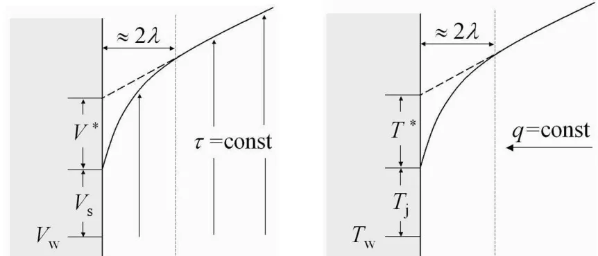
The importance of the Knudsen layer can be illustrated by the following example of low-speed, low-Kn, isothermal planar Poiseuille flow. The velocity slip (assumingα= 1.0) and Knudsen layer effects have, up until now, been usually accounted for within a NSF solution by using ‘fictitious’ (sometimes called ‘macro’) slip boundary conditions. This means the factor ζ in eq. (1) is assigned the value 1.146 [1]. This means the value of the slip velocity,V∗ in Fig. 1, is artificially increased; the resulting NSF solution is indicated by the dashed line in Fig. 1. At low Knudsen numbers, the difference between the actual velocity profile and the one generated by the NSF equations with this ‘fictitious’ velocity slip at the boundaries is small.
approximation (the stress, in fact, varies∼10% from its maximum value over the Knudsen layer thickness of ∼2λ).
Using α= 1.0, the NSF prediction for the mass flow rate, m, in this Poiseuille flow is easily calculated as [3]:
m=−2ρGh 3
3µ (1 + 3ζKn), (3)
whereGis the applied pressure gradient, andhis half the height of the flow channel. For Kn = 0.05 and using the ‘fictitious’ ζ = 1.146, the percentage increase in the mass flow rate due to slip and Knudsen layer effects is therefore ∼17% [3].
However, the actual, or ‘micro’ slip (Vs in Fig. 1) can be obtained by using a coefficient
[image:4.595.82.513.347.532.2]ζ =p2/π ≈0.8 [4]. By substituting this value into eq. (3) we can evaluate the contribu-tion to the increased mass flow rate that is solely due to velocity slip. This contribucontribu-tion is ∼70% of the change inm. Therefore the remaining∼30% must be due to the non-linear structure of the Knudsen layer.
Figure 1: Schematics of Kramer’s problem (left) and the temperature jump problem (right): VW andTW
are the velocity and temperature of the wall, respectively;VsandTjare the velocity slip and temperature
jump at the wall;V∗andT∗are the amount of ‘fictitious’ slip velocity and temperature jump that would
be required to ensure that an NSF solution (indicated by the diagonal dashed line) provides an accurate prediction beyond the Knudsen layer’s limit (which is roughly indicated by the vertical dashed line).
However, the model due to Lockerby et al. [4] introduces a scaling into the fluid’s linear constitutive relations (that is equivalent to using an ‘effective’ viscosity) so as to produce the actual strain-rate occurring in the Knudsen layer from a given stress. This constitutive-relationship scaling does not generate an artificial stress variation in the Knudsen layer; on the contrary, the modified constitutive relations ensure that the correct stress is obtained from the nonlinear strain rate within the Knudsen layer.
It is also important to note that this effective viscosity does not have an independent physical meaning; it should only be applied within the constitutive relations, and not in other relations where the transport coefficients are needed. For example, in calculating the boundary conditions given in eq. (1), the actual viscosity should be used.
While the basic principle of applying scaled constitutive relations is similar to that of a wall function approach to turbulent flow modeling [7] — and this is the reason that the name ‘wall function’ was ascribed to the model in [4] — the way in which Lockerby et al. obtained their scaled constitutive relations, and the overall aim of their model, is quite different from that of the wall function approach in turbulent flows.
Based on data from an extensive literature survey, in this present paper we describe a more reliable and accurate scaling of the constitutive relation in the NSF momentum equation outlined in [4]. While a similar process can be used to scale the constitutive relations in the energy equation in order to model the thermal Knudsen layer, we do not pursue this here for reasons of space (although we do cite the relevant literature).
Further, we identify a simple means to predict the impact of the accommodation coef-ficient,α, on the form of the momentum Knudsen layer and, consequently, on our scaling. Our scaling model is designed to be used in conjunction with the Maxwell boundary con-dition, given in eq. (1), with the slip coefficient ζ = 0.8. For surfaces with high levels of curvature there have been few detailed theoretical studies of the Knudsen layer. So, for want of a more accurate alternative, we suggest using the conventional slip coefficient value: ζ = 1.0.
3 THEORETICAL BASIS
3.1 Kramer’s problem: the momentum Knudsen layer
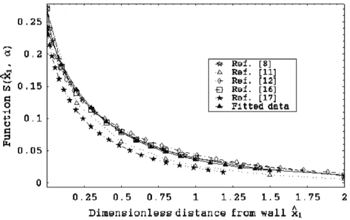
In Kramer’s problem, a uniform shear stress generates monatomic gas flow over a stationary planar wall. The flow is incompressible, isothermal, and in a direction parallel to the planar wall (as shown in Fig. 1). For this configuration, flow velocity profiles,u(ˆx1), are available in the literature [8, 11, 12, 14, 16, 17] and are of the form:
u(ˆx1) =k(ˆx1+β−S(ˆx1)), k =
du dxˆ1
¯ ¯ ¯ ¯xˆ
1→∞
(4)
where ˆx1 is the non-dimensional distance from the wall:
ˆ
x1 = √
π
2
x1
λ, (5)
β is a dimensionless slip coefficient (not to be confused with ζ in eq. (1)), and S(ˆx1) is a dimensionless function that describes the spatial structure of the momentum Knudsen layer. This latter correction function is positive for small ˆx1 and tends to zero as ˆx1 → ∞, reflecting the fact that the linear NSF constitutive relations work well for the flow outside of the Knudsen layer but not within it.
Here, we use the function S(ˆx1) to obtain the effective viscosity required to produce the appropriate scaling of the NSF constitutive relations. First, eq. (4) is differentiated and rearranged to give:
du dxˆ1
¯ ¯ ¯ ¯ˆx
1→∞
=
µ
1− dS
dxˆ1
¶−1 du dxˆ1
. (6)
Given that the stress,τ, is constant throughout the half space, and that the NSF consti-tutive relations are valid as ˆx1 → ∞ (i.e. τ =−µdu/dxˆ1|xˆ1→∞), eq. (6) can be re-stated in the following form:
τ =−
µ
1− dS
dxˆ1
¶−1 µdu
dxˆ1
, (7)
which describes the actual nonlinear relationship between stress and strain rate within the Knudsen layer. This nonlinearity can be implemented within the linear constitutive relations of the NSF equations by defining an ‘effective’ viscosity:
τ =−µeff du dxˆ1
, where µeff =
µ
1− dS
dxˆ1
¶−1
µ. (8)
3.2 An approximate expression for S
In order to obtain an expression for our effective viscosity, µeff, given in eq. (8), a
approximate expression forS. We assume, subject to later confirmation of its generality, that ln(S) varies as a linear function of ln(1 + ˆx1), so that:
S =C(1 + ˆx1) A
, (9)
where A and C are the curve-fitting coefficients. (Note: In an early attempt to combine simplicity with accuracy, we started off assuming that ln(S) varied linearly with ˆx1, but found that the fitted curves did not match the original data forS as well as the functional dependence described here. We are sure that other functional dependencies could be found that fit the available data as well, if not better. Indeed, if an analytical expression for S becomes available in the future, we would prefer to use this expression in obtaining the effective viscosity in our method.)
[image:7.595.130.472.478.693.2]In order to obtain accurate values for the coefficients in eq. (9) we have reviewed a wide range of literature relating to Kramer’s problem (and the temperature jump problem too) [8, 9, 10, 11, 12, 13, 14, 15, 16]. There are some common elements in this body of theoretical research. Most notably, in all cases the linearized Boltzmann equation and Maxwell’s microscopic boundary condition are used. There is very little experimental data yet available, and the Knudsen-layer problem has barely been touched on by the computational molecular dynamics community [3, 4]. Nonetheless, the velocity profile in Kramer’s problem, computed from kinetic theory in [8, 9, 10, 11, 12, 13, 14, 15, 16], compares very well with the results of the few reliable experimental studies (see, e.g., [17]). Figure 2 shows different results from the literature for the form of S (with an accommodation coefficient, α = 1.0); there is, generally, a very close agreement in the form and magnitude of the Knudsen layer.
The data in the literature show that for ˆx1 ≥ 1.5, S is generally small in comparison to the other two terms in the velocity profile, eq. (4). For the sake of simplicity in curve-fitting, we therefore evaluate S in the restricted range 0≤xˆ1 ≤1.5. We then obtain the following values for the fitting coefficients, with α = 1.0 for two different gas molecular models:
Hard sphere: A=−2.719, C = 0.238, (10) BGK: A=−2.025, C = 0.284.
[image:8.595.129.472.367.581.2](While some of the Kramer’s problem solutions we have cited assume the BGK molecular model, we find that in practice the difference in coefficients between hard-sphere and BGK molecules makes very little difference to the final results we report below for our scaled-NSF model.) Figure 3 shows an example of our curve-fitted expression forS compared to data from Ref. [8] for Kramer’s problem in a hard-sphere gas. As can be seen, the fit to the theoretical data is very good, with the largest error occurring very close to the wall (the maximum relative error of the expression for S is around 10%).
Figure 3: Function ln[S(ˆx1, αm= 1.0)] for Kramer’s problem in [8], and its fitted curve.
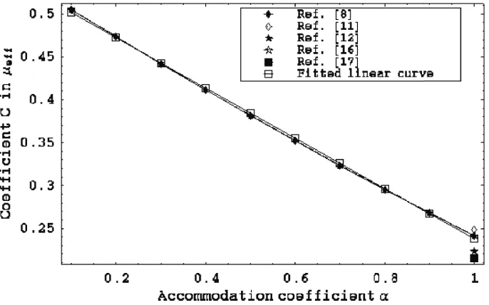
3.3 Dependence on surface accommodation
coefficients, i.e. A = A(α) and C = C(α). On investigating this dependency with our cited data from the literature, we find thatC is almost a linear function ofα (see Fig. 4):
C =Dα+E, (11)
and we then obtain the following values for the fitting coefficients:
Hard spheres: D=−0.293, E = 0.531, (12) BGK: D=−0.328, E = 0.612.
[image:9.595.129.472.294.508.2]We find, however, that the coefficient A is almost independent of the surface accommo-dation. This implies that the form and extent (into the flow) of the Knudsen layer is independent of the surface accommodation.
Figure 4: Coefficient Cfor Kramer’s problem (hard sphere molecules).
Substituting eq. (9) with eqs. (12), (11), (10), into eq. (8) provides the final expression for the effective viscosity required to reproduce the Knudsen layer structure within a NSF model,
µeff= £
1−A(Dα+E)(1 + ˆx1) A−1¤−1
µ, (13)
where the mean free path,λ, defined in eq. (2), is evaluated outside of the Knudsen layer. As ˆx1 becomes large (i.e. outside of the Knudsen layer), the effective viscosity tends to the value of the actual viscosity, meaning that away from the wall the scaling does not affect the solution in any way.
4 VELOCITY SLIP COEFFICIENT
As noted prviously, the slip coefficient ζ featuring in the Maxwell boundary condition, eq. (1), is rarely set so that it predicts the actual velocity slip and temperature jump at a gas-surface interface. Instead, it is set so that an amount of ‘fictitious’ slip is incorporated in the prediction (this fictitious slip value is labelled V∗ in Fig. 1). This ensures that the NSF constitutive relations can at least provide a good prediction of the flow field outside of the Knudsen layer. The diagonal dashed lines in Fig. 1 indicate the NSF solution that is obtained when using fictitious slip and jump slip coefficients in eq. (1).
When using our constitutive-relation scaling, however, there is no need to incorporate any artificial slip at the boundary; the actual slip boundary condition should be used. We have obtained average values for the actual velocity slip coefficient (and the temperature jump coefficient, too) from a number of different sources on Kramer’s problem and the temperature jump problem [8, 9, 10, 11, 12, 13, 14, 15, 16, 17, 18, 19, 20, 21]. For the actual velocity slip we find:
Hard spheres & BGK: ζ ≈0.8, (14)
which is in agreement with that presented in [4].
This value is for planar wall boundaries; for curved surfaces, especially if the curvature of the surface is high compared to the mean free path, this velocity slip coefficient is unlikely to be accurate. Unfortunately, only very limited work has been reported on the extent to which the velocity slip and temperature jump coefficients depend on surface curvature. This could form the basis of a useful future investigation in its own right, but in the meantime the authors suggest using the standard Maxwell slip coefficients (i.e.
ζ = 1.0) for flows in and around highly curved geometries.
5 A TEST APPLICATION: RAREFIED GAS FLOW PAST A SPHERE
In order to test the generality, and consequent usefulness, of our scaled constitutive re-lation, it needs to be applied to flow problems other than those that approximate Kramer’s problem. As a first test, we have chosen to investigate rarefied gas flow around a sphere (for an isothermal, creeping flow of a monatomic gas). The sphere is assumed to have infinite thermal conductivity, and a uniform surface temperature which is that of the free-stream gas flow. There is no condensation or evaporation in this problem (i.e. the particle is non-volatile [22, 23]).
Previous relevant kinetic-theoretical research on this problem can be found in Refs. [23, 24, 25, 26, 27, 28, 29, 30, 31, 32]. In all cases the fundamental equation studied was the linearised Boltzmann equation (or other linearised kinetic models) together with Maxwell’s microscopic boundary condition; mostly, either the BGK model or hard sphere molecular model were adopted.
reported data over a wide range of Knudsen numbers, and empirical equations to fit this experimental data are given in Refs. [34, 35]. Almost all of the work reported in these papers focuses on predicting or measuring the drag force as a function of Knudsen number in the purely diffusive boundary situation, α= 1.0.
References [23, 24] report kinetic-theoretical predictions of the variation of drag force with accommodation coefficient, α, for certain Knudsen numbers. Expressions for the drag force as a function of Kn and α have appeared in: ref. [33], based on a moment solution to the Boltzmann equation; ref. [36], from a thirteen moment analysis [35]; and ref. [37], from the traditional NSF equations with velocity slip and temperature jump boundary conditions.
From the point of view of CFD solutions, the problem can be straightforwardly set-up and solved, along with our effective viscosity model, provided that it is possible to calculate the distance from the surface of the sphere at any point in the flow. An efficient numerical way of performing this distance calculation is reported in [38]. In addition, in order to obtain the most accurate predictions of drag force (and other quantities) the numerical grid must be refined close to the surface of the sphere. Other points relating to the computational procedure are: the convergence criterion we apply is that the relative difference in the drag force between two successive numerical iterations should be less than 10−10
; as required physically, our CFD solution recovers the traditional NSF values for velocity if we setµeff =µ; since the surface of the sphere is curved, and in our investigated
range of Kn (≤ 1.0) the degree of curvature is not small, and following our discussion in a previous section above we apply the Maxwell slip coefficient, ζ = 1.0, for both the traditional NSF equations and our model.
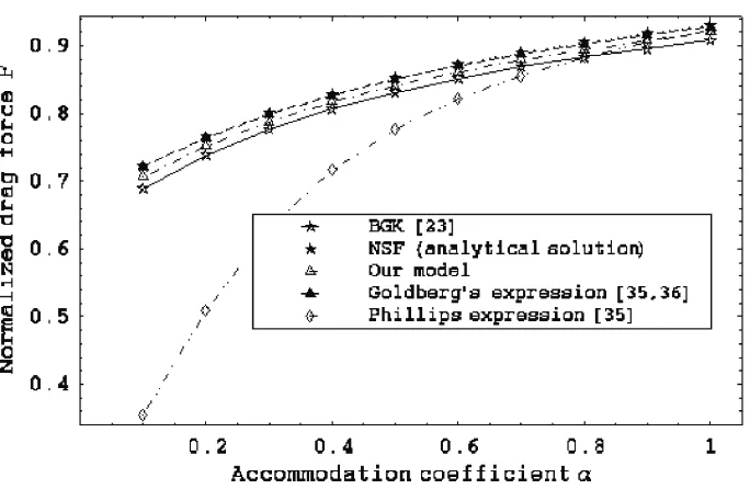
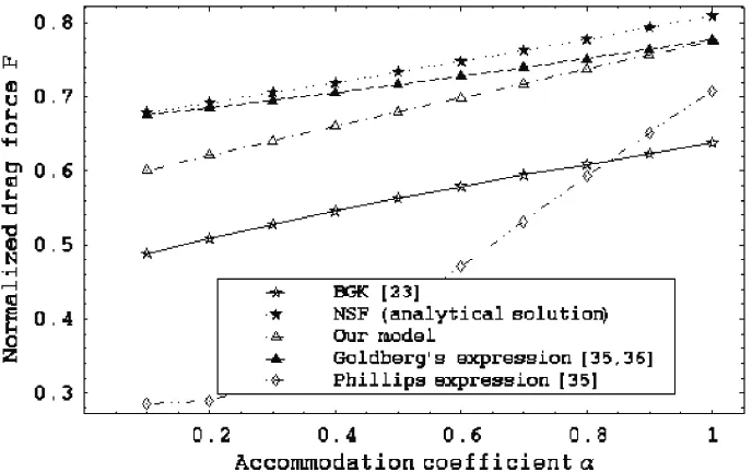
Figure 5 shows the variation of normalized drag force with Kn forα= 1.0. We see that our model gives somewhat better results for this force than the traditional NSF equations with non-scaled constitutive relations. Figures 6, 7 and 8 show the variation of normalized drag force withα for Kn = 0.1, 0.25, and 0.5. Together, these show that:
• over a range of α and Kn, our model predicts drag force results that are closer to independent kinetic-theoretical results than the traditional NSF equations predict;
• our model gives good agreement with kinetic-theoretical results for the drag up to Kn = 0.1 (with an average relative error of only 1.5%), and acceptable agreement up to Kn = 0.25 (with an average relative error of 6%);
• Goldberg’s expression from the 13 moment equations [35, 36] gives similar results to the traditional NSF equations, which are not as close to kinetic-theoretical results as the results from our model;
• Phillips’ approximate expression [35] only works well for large α (i.e. ≈ 1.0) when Kn.0.1.
Figure 5: Normalized drag force variation with Kn forα= 1.0.
[image:12.595.130.472.439.662.2]Figure 7: Normalized drag force variation withαfor Kn = 0.25.
Figure 8: Normalized drag force variation withαfor Kn = 0.5.
6 CONCLUSIONS
[image:13.595.128.472.376.592.2]from an ideal half-space flow problem: Kramer’s problem.
The advantages of our model are twofold: the flow in the Knudsen layer is described much better than when using the traditional NSF equations; and the boundary conditions remain the same as in the traditional NSF model (although the slip coefficient is changed) so there is no need to develop any of the additional boundary conditions required by higher-order hydrodynamic models for rarefied gas flows.
We applied our model to the problem of a spherical particle moving through a rarefied monatomic gas, and obtained values for the drag force. For this particular problem, our model gives much better results than the traditional NSF equations with non-scaled con-stitutive relations; excellent results are obtained for flows with Kn.0.1, and acceptable results up to Kn≈0.25.
We are investigating extending our model to non-isothermal cases, where a thermal Knudsen layer is also present; we are adopting a methodology very similar to that de-scribed here, i.e. using published kinetic-theoretical data on the half-space temperature-jump problem to scale the temperature-gradient/heat-flux relationship. Further test cases, including applying our model to, e.g., planar and cylindrical Couette flow, are also under investigation.
ACKNOWLEDGEMENTS
The authors would like to thank: Lynne O’Hare, Graham Macpherson and Simon Mizzi of the University of Strathclyde, UK; Robert Barber and David Emerson of Daresbury Laboratory, UK; Rho Shin Myong of Gyeongsang National University, South Korea. This work is funded in the UK by the Engineering and Physical Sciences Research Council under grant no. GR/S77196/01, by a Visiting Fellowship for YZ from the Leverhulme Trust under grant no. F/00273/G, and through a Philip Leverhulme Prize for JMR from the Leverhulme Trust.
REFERENCES
[1] C. Cercignani. Rarefied gas dynamics: from basic concepts to actual calculations, Cambridge University Press (2000).
[2] J.M. Reese, M.A. Gallis and D.A. Lockerby. New directions in fluid dynamics: non-equilibrium aerodynamic and microsystem flows. Philosophical Transaction of the Royal Society, A,361, 2967–2988 (2003).
[3] D.A. Lockerby, J.M. Reese and M.A. Gallis. The usefulness of higher-order constitu-tive relations for describing the Knudsen layer.Physics of Fluids,17, 100609 (2005).
[5] J.C. Maxwell. On stresses in rarified gases arising from temperature inequalities. Philosophical Transactions of the Royal Society of London,170, 231–256 (1879).
[6] M. von Smoluchowski. ¨Uber w¨armeleitung in verd¨unnten gasen.Annalen der Physik und Chemie, 64, 101–130 (1898).
[7] S.B. Pope. Turbulent Flow, Cambridge University Press (2000).
[8] M. Wakabayashi, T. Ohwada and F. Golse. Numerical analysis of the shear and thermal creep flows of a rarefied gas over the plane wall of a Maxwell-type boundary on the basis of the linearized Boltzmann equation for hard-sphere molecules.European Journal of Mechanics B/Fluids, 15, 175–201 (1996).
[9] Y. Sone, T. Ohwada and K. Aoki. Temperature jump and Knudsen layer in a rarefied gas over a plane wall: Numerical analysis of the linearized Boltzmann equation for hard-sphere molecules. Physics of Fluids A, textbf1, 363–370 (1989).
[10] S.K. Loyalka. Temperature jump: Rigid-sphere gas with arbitrary gas/surface inter-action. Nuclear Science and Engineering, 108, 69–73 (1991).
[11] S.K. Loyalka and H.A. Hickey. Velocity slip and defect: Hard sphere gas. Physics of Fluids A, textbf1, 612–614 (1989).
[12] S.K. Loyalka. Velocity profile in the Knudsen layer for the Kramer’s problem.Physics of Fluids,18, 1666–1669 (1975).
[13] C.E. Siewert. The linearized Boltzmann equation: a concise and accurate solution of the temperature-jump problem. Journal of Quantitative Spectroscopy and Radiative Transfer,77, 417–432 (2003).
[14] C.E. Siewert. Kramers’ problem for a variable collision frequency model. European Journal of Applied Mathematics, 12, 179–191 (2001).
[15] L.B. Barichello, A.C.R. Bartz, M. Camargo and C.E. Siewert. The temperature-jump problem for a variable collision frequency model.Physics of Fluids,14, 382–391 (2002).
[16] C.E. Siewert. The linearized Boltzmann equation: Concise and accurate solutions to basic flow problems. ZAMP, textbf54, 273–303 (2003).
[18] M.A. Reynolds, J.J. Smolderen and J.F. Wendt. Velocity profile measurements in the Knudsen layer for the Kramers problem. In Proceedings of the Ninth International Symposium of Rarefied Gas Dynamics, M. Becker and M. Fiebig, eds., Dfvlr-Press (1974).
[19] N.J. McCormick. Gas-surface accommodation coefficients from viscous slip and tem-perature jump coefficients. Physics of Fluids, 17, 107104 (2005).
[20] T. Klinc and I. Kuscer. Slip coefficients for general gas-surface interaction. Physics of Fluids,15, 1018–1022 (1972).
[21] C.E. Siewert. The temperature-jump problem based on the CES model of the lin-earized Boltmann equation. ZAMP, 55, 92–104 (2004).
[22] Y. Sone, S. Takata and M. Wakabayashi. Numerical analysis of a rarefied gas flow past a volatile particle using the Boltzmann equation for hard-sphere molecules. Physics of Fluids,6, 1914–1928 (1994).
[23] S.A. Beresnev, V.G. Chernyak and P.E. Suetin. Motion of a spherical particle in a rarefied gas. Part 1. A liquid particle in its saturated vapour. Journal of Fluid Mechanics, 176, 295–310 (1987).
[24] S.A. Beresnev, V.G. Chernyak and G.A. Fomyagin. Motion of a spherical particle in a rarefied gas. Part 2. Drag and thermal polarization. Journal of Fluid Mechanics, 219, 405–421 (1990).
[25] S. Takata and Y. Sone. Flow induced around a sphere with a non-uniform surface temperature in a rarefied gas, with application to the drag and thermal force problems of a spherical particle with an arbitrary thermal conductivity. European Journal of Mechanics, B/Fluids, 14, 487–518 (1995).
[26] S. Takata, Y. Sone and K. Aoki. Numerical analysis of a uniform flow of a rarefied gas past a sphere on the basis of the Boltzmann equation for hard sphere molecules. Physics of Fluids, A,5, 716–737 (1993).
[27] Y. Sone and K. Aoki. Slightly rarefied gas flow over a specularly reflecting body. Physics of Fluids, 20, 571–576 (1977).
[28] S.K. Loyalka. Motion of a sphere in a gas: Numerical solution of the linearized Boltzmann equation. Physics of Fluids, A, 4, 1049–1056 (1992).
[30] K.C. Lea and S.K. Loyalka. Motion of a sphere in a rarefied gas. Physics of Fluids, 25, 1550–1557 (1982).
[31] C. Cercignani, C.D. Pagani and P. Bassanini. Flow of a rarefied gas past an axisym-metric body. II. Case of a sphere. Physics of Fluids,11, 1399–1403 (1968).
[32] D.R. Willis. Sphere drag at high Knudsen number and low Mach number.Physics of Fluids, 9, 2522–2524 (1966).
[33] R.A. Millikan. The general law of fall of a small spherical body through a gas, and its bearing upon the nature of molecular reflection from surfaces. The Physical Review, 22, 1–23 (1923).
[34] M.D. Allen and O.G. Raabe. Re-evaluation of Millikan’s oil drop data for the motion of small particles in air. Journal of Aerosol Science, 13, 537–547 (1982).
[35] W.F. Phillips. Drag on a small sphere moving through a gas. Physics of Fluids, 18, 1089–1093 (1975).
[36] R. Goldberg. The flow of a rarefied perfect gas past a fixed spherical obstacle, PhD thesis, New York University (1954).
[37] R.W. Barber and D.R. Emerson. Analytical solution of low Reynolds number slip flow past a sphere, Daresbury Laboratory (UK) Technical Report, DL-TR-2000-001 (2000).
![Figure 3: Function ln[S(ˆx1, αm = 1.0)] for Kramer’s problem in [8], and its fitted curve.](https://thumb-us.123doks.com/thumbv2/123dok_us/1716795.125072/8.595.129.472.367.581/figure-function-x-am-kramer-problem-tted-curve.webp)