Performance Indicators in Agricultural Financial Markets Factor Markets Working Document No 43, May 2013

FACTOR MARKETS Working Papers present work being conducted within the FACTOR MARKETS research project, which analyses and compares the functioning of factor markets for agriculture in the member states, candidate countries and the EU as a whole, with a view to stimulating reactions from other experts in the field. See the back cover for more information on the project. Unless otherwise indicated, the views expressed are attributable only to the authors in a personal capacity and not to any institution with which they are associated.

Available for free downloading from the Factor Markets (www.factormarkets.eu) and CEPS (www.ceps.eu) websites

ISBN 978-94-6138-312-9

© Copyright 2013 Kristina Hedman Jansson and Carl Johan Lagerqvist  

FACTOR MARKETS Coordination: Centre for European Policy Studies (CEPS), 1 Place du Congrès, 1000 Brussels, Belgium Tel: +32 (0)2 229 3911 • Fax: +32 (0)2 229 4151 • E-mail: [email protected] • web: www.factormarkets.eu

Performance Indicators in Agricultural

Financial Markets

ABSTRACT

This study attempts to develop performance indicators for the financial markets based on the findings in an earlier Factor Markets Working Paper (No. 33, “Agricultural credit market institutions: A comparison of selected European countries”) and on FADN (Farm Accountancy Data Network) data. Two indicators were developed. One measured the long-term economic sustainability of agricultural firms since the financial characteristics of the firms were perceived as important factors when rejecting a loan applicant. If the indicator works, it should show that a low value in this indicator is related to the performance in the financial markets. The second indicator was the loan-to-value (LTV), or debt-to-asset ratio, the reasoning behind this indicator is that low values can point to credit constraints, and in WP 33 we saw that the interviewed experts expected LTVs to be much higher than what is actually the case. We find that the first indicator can’t be used to measure the performance of the financial institutions, since we can’t show any relationship between the indicator and activities in the financial markets. However, the indicator is valuable for its measurement of the long-term financial sustainability of the agricultural sector, or of the firms. The loan-to-value indicator does imply that most countries would have room to increase the credit.

No. 43, May 2013

1. Introduction ... 1

2. Performance indicators ... 2

2.1 Room for consumption – economic sustainability ... 2

2.2 Loan to value ... 5

3. Farm structure in the case study countries and connection to the indicators ...8

3.1.1 Farm structure typology ...8

3.2 Farm structure and performance indicators ... 10

3.2.1 Room for consumption – economic sustainability ... 10

3.2.2 Loan to value – debt to asset ratio ...11

4. Performance indicators and government support ... 12

5. Conclusions ... 13

References ... 15

Appendix 1. Stepwise calculations for all countries ... 16

List of Tables

Table 2. Economic sustainability in the case study countries (subsidies included). ... 4

Table 3. Room for consumption in relation to GDP/capita ... 5

Table 4. Development of land prices in the case study countries ...8

Table 5. National average prices of agricultural land in some of the case study countries ...8

Table 6. Farm structures in the case study countries (2007) ... 9

Table 7. Livestock domination, share of livestock output in total output ... 9

Table 8. Farm structure typology ... 10

Table 9. Fluctuations in room for consumptions, ordered from smallest to largest ...11

Table 10. LTV and production type ...11

Table 11. LTV and farm structure – average farm size ...11

Table 12. Government involvement in the agricultural credit markets ... 12

List of Figures

Figure 2. LTV of fixed capital... 7

|1

Financial Markets

Kristina Hedman Jansson and Carl Johan Lagerqvist

Factor Markets Working Paper No. 43/May 2013

1.

Introduction

In this Working Paper some of the findings of Jansson et al (2013) (WP 33 of the Factor Markets project, Agricultural credit market institutions: A comparison of selected European countries, hereinafter WP 33) have been the starting point to develop economic and financial performance indicators.

In WP33 we found agricultural specific involvement of government in financial markets which might indicate that the governments assume that agriculture has problems in receiving credit. Different levels of involvement were found: agriculture specific regulations (FYROM, Italy and France), different kinds of government support (Finland, Netherlands, Greece, Germany, Italy, France and Belgium) and the existence of government credit institutions (all case study countries except Ireland, UK, Slovakia and Sweden). At least the various types of government support have been shown to be inefficient (Swinnen & Gow, 1999). Another indication of inefficiencies in the agriculture financial markets is the low values of LTV. In Curtiss (2012) this is mentioned as a sign of credit constrains.

Our first indicator draws on WP 33 where we found that economic factors, such as farm business income, credit history and access to collateral were important factors in credit rejections. Furthermore, if a firm shall be long-term sustainable (in economic terms) there needs to be enough room for household consumption and taxes so the farmer can make a living off the firm. In the current WP we develop an indicator to measure the economic sustainability (ES) of the farm. We assume that farms with low values in ES are likely to have difficulties in receiving loans.

The second indicator is loan to value (LTV), or debt-to-asset ratio. In WP 33 we found that the experts who were interviewed for the questionnaire consistently expected the level of LTV to be higher than what the calculations of LTV implied. The LTV also provides a measure of how much collateral is available, although most countries were shown to lean towards cash-flow-based lending rather than asset-based lending. To further investigate this, in the current WP we use FADN data to calculate the LTV’s for the case study countries and compare them to the expected levels that were reported in WP 33.

The questions we seek to answer are:

1) Can ES be used as a performance indicator of the financial markets? In other words, is there a connection between ES and the situation on the financial markets for the agricultural firms?

2) Is LTV lower that what the experts expected in WP 33? Does this imply that the credit levels could be higher in agriculture?

Differences in economic performance and LTV might be explained by differences in farm structure and production. We use FADN and FSS (Farm structure statistics) data from Eurostat to describe the farm and production structures of the case study countries to see if it is possible to explain differences in the performance indicators.

∗ _{Kristina Hedman Jansson and Carl Johan Lagerqvist are are researchers at Sveriges}

For the indicator development, FADN data (online version) was used. This clearly reduced the possibilities to do detailed indicators since the online version is aggregated at national level. A drawback with using FADN data in this working paper is also that FYROM is not included in the data set and we thus lose one of the case study countries.

2.

Performance indicators

2.1

Room for consumption – economic sustainability

In Working Paper No. 33 we saw that an important factor in the risk assessment of banks is the economic situation of the firm (see Table 8, p. 11 in WP No. 33). Examples of important factors for rejecting a loan applicant are: “Insufficient farm business income”, “Poor credit history of the applicant” and “Lack of collateral”. When it comes to weights assigned to different characteristics in risk assessment (see Table 10, p.13 in WP No. 33) high weight is given to cash flow. All of these are related to the economic and financial situation of the farms and we thus conclude that an indicator to measure the economic sustainability of a firm could give an insight into the likelihood for firms to get credit in the long run. Furthermore, household income also influences the credit constraints: a higher household income reduces the risk of experiencing credit constraints, either through the demand for credit being lower in a higher-income household or through the creditor perceiving the investment to be more secure (Nuryartono et al., 2005). Similar results are also found in Rahji & Adeoti (2010). In Lagerkvist, 2001, a model is presented to analyse the economic performance of firms, based on financial statement data like the data in FADN. Based on that model we build an indicator of economic sustainability based on what the farmer has left for private consumption and taxes after all costs have been covered. We thereafter relate that room for consumption to the GDP per capita (euro) to enable comparison between countries. Economic sustainability (ES) is calculated as

ES=I-(ΔF+ΔD)

Where (I) is net cash income, (ΔF) is change in funds used between years, and (ΔD) is change in debt use between years.

Table 1. Data description

Item Calculation Data description

Farm income Total Output (SE131) + Total Subsidies – excluding on investments (SE605)-Total Input (SE270)

SE131 = Total of output of crops and crop products, livestock and livestock products and of other output. Sales and use of (crop and livestock) products and livestock + change in stocks of products (crop and livestock) + change in valuation of livestock - purchases of livestock + various non-exceptional products. (incl. Leased land ready for sowing, receipts from occasional letting of fodder areas, agistment, forestry products, contract work for others, hiring out of equipment, interest on liquid assets necessary for running the holding, receipts of tourism, receipts relating to previous accounting years, other products and receipts)

SE605 = Subsidies on current operations linked to production (not investments). Payments for cessation of farming activities are therefore not included. Entry in the accounts is generally on the basis of entitlement and not receipt of payment, with a view to obtain coherent results (production/costs/subsidies) for a given accounting year. SE270 = Specific costs + Overheads + Depreciation + External factors. Costs linked to the agricultural activity of the holder and related to the output of the accounting year. Included are amounts relating to inputs produced on the holding (farm use) = seeds and seedlings and feed for grazing stock and granivores, but not manure. When calculating FADN standard results, farm taxes and other dues are not included in the total for costs but are taken into account in the balance Subsidies and taxes (subsidies - taxes) on current and non-current operations. The personal taxes of the holder are not to be recorded in the FADN accounts (including remuneration of inputs (work, land and capital) which are not the property of the holder. = wages, rent and interest paid.)

Current farm

assets Total current assets (SE465) Calculated as a change (=year n- year (n-1))

SE465 = Non-breeding livestock + Circulating capital (Stocks of agricultural products + Other circulating capital).

Long term

farm assets Total fixed assets (SE441) Calculated as a change (=year n- year (n-1))

SE441 = agricultural land and farm buildings and forest capital + buildings + Machinery and equipment + Breeding livestock. Funds available for withdrawals and taxes Calculate(Income-Change in assets)

Actual change

in debt use Long-term (SE490) + Short term (SE495) debt. Calculated as a change (=year n- year (n-1))

SE490 = Loans contracted for a period of more than one year.

SE495 = Loans contracted for less than one year and outstanding cash payments.

Room for

Table 2. Economic sustainability in the case study countries (subsidies included).

BE DE GR FR IE IT NL PL FI SE SK UK 1990 18707 19408 7769 13712 10022 4417 26159 29780

1991 30797 1423 9568 24249 10761 357 13642 30546

1992 -13123 -11596 5944 2902 5280 6940 -24035 78725

1993 18748 11138 8813 28339 18143 23987 -45068 23054

1994 1814 -4707 7822 8087 -3029 -77634 -28909 -21211

1995 24124 -256725 8327 13517 -1046 20039 -2730 -178910 -404059 18579

1996 33987 35773 4976 11832 -9418 -12348 28184 19046 -14048 -3790

1997 42759 47312 7190 23387 -13373 4580 1220 17795 21870 -143670

1998 31151 643 11872 20053 -5682 -34263 -54226 -37762 -11047 26749

1999 6459 -69571 7655 2594 -27802 6337 -159434 -16920 -19962 -32332

2000 44632 33274 10744 18510 -52697 19744 -213373 10716 -71418 -19895

2001 46578 12602 6296 32563 -9682 16363 -242144 14164 17479 -105147

2002 19717 3802 10742 6188 -60949 -84195 -43611 21718 -78131 37964

2003 13017 9516 8394 24465 39556 117446 17404 5189 -11872 103233

2004 10154 5095 6582 -957 -39804 41509 -63494 -1891 -31765 -3917

2005 33432 26105 10198 27795 -165730 -23657 -92407 2354 -18254 -106015 -58291 -108496

2006 5891 -11006 8524 11803 -168057 12096 -12987 2252 -10543 -67650 319461 -76206

2007 -14884 34658 11992 26212 -68751 22625 -107613 -2087 -6815 30712 -257981 -146285

2008 1230 10840 12090 4112 75215 46200 -95711 -4925 -4286 934 412954 155911

2009 40325 15849 7081 27251 101161 27621 -175376 -25130 9859 69398 -1283712 -7959

STDEV 18361 64205 2093 10252 65303 42848 80414 11392 17132 48172 678218 78581

Source: Own calculations based on FADN. Calculations for individual countries can be found in Appendix 1,

Stepwise calculations for all countries. 

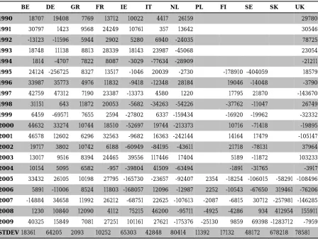
When investigating further what the determining factors are in the ES indicator it is helpful to look at the stepwise calculations of the indicator (Appendix 1). A year with a mediocre income could turn out to give a high value in ES if the change in assets is negative (selling or depreciation) and the change in debts is positive (increasing the debts from one year to another). And this is also what we can see in the stepwise calculations. The negative years for most countries are mainly caused by a strong positive change in assets, in the case of Belgium 2007 was extreme, for Germany 1995 was extreme and for France 2004 was extreme.

For most countries the increase in assets is mirrored by an increase in debt (see Graphs in appendix 1) with the exceptions of Greece, Italy, Ireland, Poland and Slovakia.

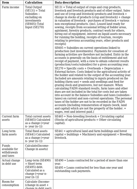
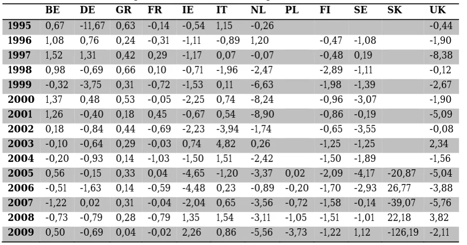
In general the room for consumption and taxes has decreased between 1995 and 2009; in most countries it is lower than the GDP/capita (see Table 3). Slovakia seems to have farmers who are economically much better off compared to national GDP/capita some years, and some years the farmers are much worse off than the national income. The FADN sample from Slovakia consists of extremely large farms; maybe this is an explanation for the extreme numbers.

Table 3. Room for consumption in relation to GDP/capita

BE DE GR FR IE IT NL PL FI SE SK UK 1995 0,67 -11,67 0,63 -0,14 -0,54 1,15 -0,26 -0,44

1996 1,08 0,76 0,24 -0,31 -1,11 -0,89 1,20 -0,47 -1,08 -1,90

1997 1,52 1,31 0,42 0,29 -1,17 0,07 -0,07 -0,48 0,19 -8,38

1998 0,98 -0,69 0,66 0,10 -0,71 -1,96 -2,47 -2,89 -1,11 -0,12

1999 -0,32 -3,75 0,31 -0,72 -1,53 0,11 -6,63 -1,98 -1,39 -2,67

2000 1,37 0,48 0,53 -0,05 -2,25 0,74 -8,24 -0,96 -3,07 -1,90

2001 1,26 -0,40 0,18 0,45 -0,67 0,54 -8,90 -0,86 -0,19 -5,09

2002 0,18 -0,84 0,44 -0,69 -2,23 -3,94 -1,74 -0,65 -3,55 -0,08

2003 -0,10 -0,64 0,29 -0,03 0,74 4,82 0,26 -1,25 -1,25 2,34

2004 -0,20 -0,93 0,14 -1,03 -1,50 1,51 -2,42 -1,50 -1,89 -1,56

2005 0,56 -0,15 0,33 0,04 -4,65 -1,20 -3,37 0,02 -2,09 -4,17 -20,87 -5,04

2006 -0,51 -1,63 0,14 -0,59 -4,48 0,23 -0,89 -0,20 -1,70 -2,93 26,77 -3,88

2007 -1,22 0,02 0,31 -0,04 -2,04 0,65 -3,56 -0,72 -1,58 -0,14 -39,07 -5,76

2008 -0,73 -0,79 0,28 -0,79 1,35 1,54 -3,11 -1,05 -1,51 -1,01 22,18 3,82

2009 0,50 -0,69 0,04 -0,02 2,26 0,86 -5,56 -3,73 -1,22 1,12 -126,19 -2,11

Source: Own calculations based on FADN.

2.2

Loan to value

The questionnaire gave somewhat contradicting results regarding the loan to value (LTV) of the agricultural sector. The experts generally estimated the LTV to be 50-90%, but when calculated the LTV was much lower at 2-50%. Here we follow up with a LTV calculation based on FADN data. A low LTV might indicate some degree of credit rationing – however, it might very well be that the farmers have borrowed as much capital as they need. But a low value still indicates that there is room for more borrowing, should the firm want to.

Loan to value has been calculated as: Total liabilities/Total assets

Figure 1. Loan to value (LTV)

Source: Own calculations based on FADN.

The results show that LTV is lower than what the experts expected in the WP 33 (p. 18-19). Some countries – Greece, Italy, Ireland, Slovakia, and Poland have LTV of 10% or less. In these countries the expected LTV as described in WP 33 were, depending on the asset: 70-90% (Greece), 30-70% (Slovakia) and 80-100% (Poland), there were no response on this question for Italy and Ireland. UK and Germany have LTVs of 10-20%. In WP 33 the experts expected the LTV to be 70-100% for the UK; there was no answer from Germany on this question. The rest of the countries all have LTV above 20%, with the highest value for Netherlands and France at about 40%. In WP 33 there were answers from Sweden (40-75%), Finland (60-100%) and the Netherlands (100%). This either indicates that there is room for more credit or means that the definitions of LTV that the experts used is not the total liabilities divided by the total assets. The discrepancy between what is calculated and what the experts expected could be caused by the experts assuming LTV for one future investment, rather than the debt-to-asset ratio.

These low LTV’s, or low debt-to-asset ratios are also pointed out in Curtiss, 2012. This could be explained by differences in accounting standards in agriculture and in non-agriculture, but also by the characteristics of the assets making them harder to liquidize. Thus, it can be difficult for the farmer to use assets as collateral for several reasons: in proprietary farms there is a lack of differentiation between business assets and private assets and the farmer’s machinery is not always possible to liquidize on a second-hand market. In other words: not all assets in a farm would be possible to use as collateral. In Weber & Musshoff (2012), they show that the risk of credit rationing is somewhat higher in agriculture than in other sectors, measured as the “probability of receiving a loan”. Although once they receive loans, they are not volume-rationed.

Another aspect of LTV is that it can show the availability of collateral. Collateral can be used to reduce the risk since the creditor can sell the collateral should the borrower default on the loan. However, as stated above, the use of collateral in agriculture is not without difficulties

0% 5% 10% 15% 20% 25% 30% 35% 40% 45%

1989 1990 1991 1992 1993 1994 1995 1996 1997 1998 1999 2000 2001 2002 2003 2004 2005 2006 2007 2008 2009

(BEL) Belgium (DEU) Germany (ELL) Greece (FRA) France

(IRE) Ireland (ITA) Italy (NED) Netherlands (POL) Poland

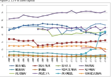
and the LTV for different asset categories are likely to differ: it is more likely to find high LTVs on land and buildings than on machinery. In mortgage loans collateral is real property, but only Sweden has mortgage institutes as an important creditor in WP 33. Most countries have commercial banks as the most important loan provider. In the Netherlands and Poland farmers’ cooperative banks are most important. Nevertheless, also these creditors might prefer fixed assets as collateral rather than cash.1 _{So an additional LTV for only fixed capital} was calculated to see if a different picture emerges from that, and to see if there still seem to be room for more credit. The results are displayed in Figure 2. It is a similar pattern, though as might be expected the LTVs are higher: Ireland, Italy Greece and Poland are still below 10% in LTV, Slovakia increases to above 30%. UK and Germany remains between 10-20%. Belgium, Sweden, Finland, and the Netherlands remain between 30 and 40%, whereas France leaps to over 60% in LTV when only the fixed assets are used. This might indicate that there is room to use fixed assets as collateral to a larger extent.

Figure 2. LTV of fixed capital

According to WP 33 one of the most important factors for rejecting a loan is the lack of collateral. The LTV indicators show that there is room for higher credits, if only the availability of fixed assets for collateral is considered. The weights assigned to different characteristics in WP 33 show that both the expected cash-flow of the investment and the availability of collateral are important, when looking at the importance of just those two – asset-based lending versus cash-flow based lending – cash flow is more important than assets in most countries (the exception being Poland).

Different types of asset will have different levels of LTV and important in determining the asset value and thus also the LTV is the land prices and the development of land prices. In

1 _{Curtiss (2012) also mentions how small firms, which are common in agriculture, usually already have}

used their own capital before turning to financial institutions for credit; thus cash as collateral would be unusual.

0% 10% 20% 30% 40% 50% 60% 70%

1989 1990 1991 1992 1993 1994 1995 1996 1997 1998 1999 2000 2001 2002 2003 2004 2005 2006 2007 2008 2009

(BEL) Belgium (DEU) Germany (ELL) Greece (FRA) France

(IRE) Ireland (ITA) Italy (NED) Netherlands (POL) Poland

Ciaian et al. (2012), the development of land prices in EU member states is described for the period 1996-2009. Among the case study countries of the current WP, Germany and Greece saw decreasing land prices, and France and Italy saw stable land prices. Increasing land prices were experienced in the Netherlands, Belgium, Ireland, Finland, Sweden, UK, Slovakia and Poland.

Table 4. Development of land prices in the case study countries

Development Country Decreasing land prices Germany, Greece Stable land prices France, Italy

Increasing land prices Netherlands, Ireland, Finland, Sweden, Belgium, UK, Slovakia & Poland

Source: Ciaian et al (2012). Time periods are 1996-2009 for old member states and 2004 to 2009 for new

member states.

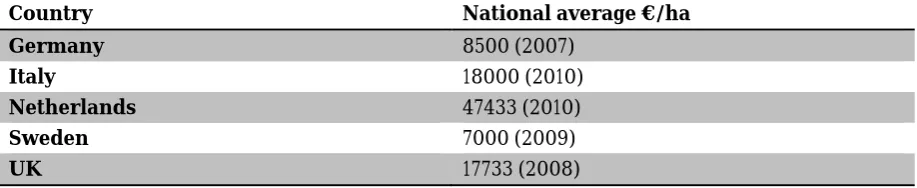
The price levels differ a lot between as well as inside the countries (Ciaian et al., 2012) (see Table 5). A farmer in an expensive region who wishes to expand is faced with high costs, but also holds an attractive asset that the creditor can use as collateral because of strong demand from alternative uses. The total asset value of the firm is also higher. In a country with low price levels, one problem might be that the farmer’s main asset is not valued high enough to be used as collateral and he will then have to rely more on cash flow to receive capital for investments.

Table 5. National average prices of agricultural land in some of the case study countries

Country National average €/ha

Germany 8500 (2007)

Italy 18000 (2010)

Netherlands 47433 (2010)

Sweden 7000 (2009)

UK 17733 (2008)

Source: Ciaian et al. (2012).

In Greece the prices vary between €4,500 and €18,000 per hectare. In France, the quality label wine regions have very high prices (€95,200/ha), whereas pastures cost about €5,000/ha. In Belgium the average prices for arable land in Flanders are considerably higher at over €15,000/ha than in Wallonia at €6,500/ha (Ciaian et al., 2012).

3.

Farm structure in the case study countries and connection to the

indicators

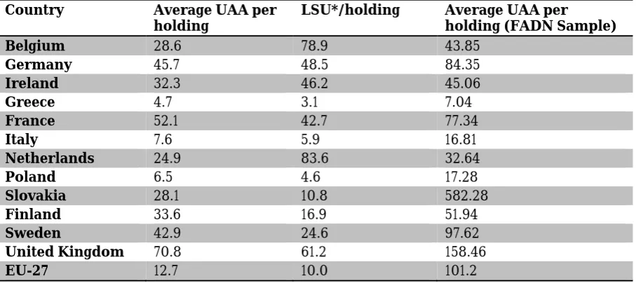
The differences in the indicators might be related to the farm structure and the production in the individual countries. We use data from the farm structure survey (FSS) and FADN to build a typology based on the structure of the agriculture in our case study countries.

3.1.1

Farm structure typology

Table 6. Farm structures in the case study countries (2007)

Country Average UAA per holding

LSU*/holding Average UAA per

holding (FADN Sample) Belgium 28.6 78.9 43.85

Germany 45.7 48.5 84.35

Ireland 32.3 46.2 45.06

Greece 4.7 3.1 7.04

France 52.1 42.7 77.34

Italy 7.6 5.9 16.81

Netherlands 24.9 83.6 32.64

Poland 6.5 4.6 17.28

Slovakia 28.1 10.8 582.28

Finland 33.6 16.9 51.94

Sweden 42.9 24.6 97.62

United Kingdom 70.8 61.2 158.46

EU-27 12.7 10.0 101.2

* LSU = Livestock units.

Source: Eurostat, 2013, FADN and own calculations.

If we look at to what extent livestock dominates production in the countries (Table 7), we see that livestock production dominates the output in most countries; the big exceptions are Greece, Italy and Slovakia, with values of about 30%. In most countries, the domination of livestock is (to a varying degree) decreasing in the period, with one interesting exception: Greece. The strongest decrease occurred in Sweden, Finland and the Netherlands.

Table 7. Livestock domination, share of livestock output in total output

BE DE GR FR IE IT NL PL SF SE SK UK 2009 56% 52% 28% 43% 79% 28% 39% 48% 54% 46% 31% 51%

2008 59% 51% 26% 41% 80% 27% 42% 47% 55% 46% 30% 50%

2007 56% 50% 22% 39% 86% 29% 40% 43% 48% 42% 31% 49%

2006 56% 50% 26% 42% 87% 32% 40% 46% 53% 50% 39% 50%

2005 58% 52% 21% 43% 87% 32% 44% 50% 57% 50% 34% 51%

2004 59% 52% 21% 43% 86% 31% 45% 49% 57% 50% 35% 52%

2003 55% 51% 21% 42% 85% 33% 40% 59% 54% 50%

2002 60% 52% 20% 42% 85% 33% 42% 57% 58% 52%

2001 64% 53% 22% 43% 86% 33% 43% 61% 60% 55%

2000 65% 57% 21% 43% 86% 32% 52% 59% 60% 52%

1999 63% 53% 22% 41% 85% 31% 51% 58% 61% 51%

1998 61% 51% 20% 42% 87% 32% 49% 58% 62% 50%

1997 64% 54% 19% 44% 90% 32% 54% 55% 63% 55%

1996 66% 54% 17% 43% 88% 32% 55% 56% 61% 57%

1995 65% 55% 18% 45% 87% 33% 51% 68% 65% 54%

1994 65% 57% 20% 47% 87% 34% 52% 55%

1993 65% 57% 20% 47% 89% 33% 54% 59%

1992 65% 56% 19% 43% 86% 31% 54% 56%

1991 67% 58% 18% 42% 84% 29% 53% 54%

1990 67% 57% 21% 43% 85% 33% 53% 52%

1989 69% 59% 20% 44% 86% 34% 56% 54%

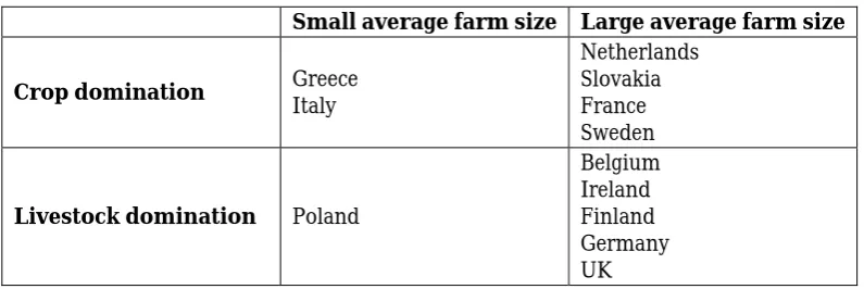
Based on the above factors we build our typology based on farm size, where the average for EU-27 is the limit between small and big farms and on livestock domination, where 50% and above means the country is dominated by livestock (Table 8).

Table 8. Farm structure typology

Small average farm size Large average farm size

Crop domination Greece _Italy

Netherlands Slovakia France Sweden

Livestock domination Poland

Belgium Ireland Finland Germany UK

The production structure contains more information: the dominating crop in total crop output in Greece is olive oil and olives and in Italy it is wine and grapes. The crops in Netherlands are mainly vegetables and flowers. In Slovakia, France and Sweden, the dominating crop is cereals. For livestock production the dominating produce in the output of livestock products are pigmeat in Poland and Belgium, beef and veal in Ireland and in Finland, Germany and the UK, cows’ milk and milk products are dominating the output.

3.2

Farm structure and performance indicators

3.2.1

Room for consumption – economic sustainability

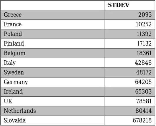
We would expect small farms to typically have small numbers in economic terms and they would probably have incomes below the national average, implying a need for off-farm income. A large farm would on the other hand have large numbers, and they might have an income closer to the national average. Based on our typology we would expect Greece, Italy and Poland, to have small numbers and incomes below the national average. In Table 9, we see that this expectation does not hold. Greece does have small, but positive numbers, Italy on the other hand, has in the worst year (2001) an income almost 9 times lower than the national average, and the best year (2003) close to 5 times higher than the national average. Also in Poland the numbers varies.

Greece, France and Belgium had good results for the ES indicator; Greece has positive results for all years, and France and Belgium had only a few negative years. Looking at the typology we can see no similarities between these three countries.

Italy and Germany also have a few negative years (5 out of 20); they also have no similarities in the farm structure typology. The countries with a majority of negative years: Ireland, Netherlands, Sweden, Finland, Poland and Slovakia also show little similarities; Netherlands, Sweden and Slovakia have big farms and are dominated by crop production. In addition the crop output in Netherlands is to a large extent (about 70%) dominated by vegetables and flowers. Sweden and Slovakia is mainly producing cereals. Poland has small average farm sizes and is dominated by livestock, and Finland has big average farm size and is dominated by livestock.

Table 9. Fluctuations in room for consumption, ordered from smallest to largest

STDEV

Greece 2093

France 10252

Poland 11392

Finland 17132

Belgium 18361

Italy 42848

Sweden 48172

Germany 64205

Ireland 65303

UK 78581

Netherlands 80414

Slovakia 678218

3.2.2

Loan to value – debt to asset ratio

In general we would expect the highest investments to be in countries where livestock is dominating output – mainly this would be the case in countries dominated by Cow milk and milk products in the output. This would mean that Poland, Belgium, Ireland, Finland, Germany and the UK would have high assets, and possibly high debts, in particular this would be expected in Finland, Germany and the UK due to the cow milk production. We would furthermore expect that small farms (Greece, Italy and Poland), might have bigger difficulties in receiving loans and thus have low LTV’s. It might also be that large farms, regardless of production structure, would have high LTV’s since they would have less difficulty than small farms to receive loans.

Again, the expected pattern does not emerge from the material we have (see Tables 10 and 11). The only expectations being fulfilled are the small farm size countries (Italy, Greece, Poland) also having low levels of LTV. Regarding the production type, Greece and Italy follow the expected pattern and show low levels of LTV.

Table 10. LTV and production type

Expected Observed

High Finland, Germany and the UK France and Netherlands,

Medium-high: Poland, Belgium, Ireland, Sweden, Finland, Belgium

Medium-low: Germany, UK, Slovakia and Poland

Low: Greece, Italy, France, Netherlands,

Sweden, Slovakia, Ireland, Greece, and Italy

Table 11. LTV and farm structure – average farm size

Expected Observed

High Netherlands, Slovakia, France, Sweden,

Belgium, Ireland, Finland, Germany, UK France and Netherlands,

Medium-high: Sweden, Finland, Belgium

Medium-low:

Germany, UK, Slovakia and Poland

4.

Performance indicators and government support

A high involvement of government in the credit market might indicate that they perceive the credit market for agriculture to be inefficient. In WP 33 (Tables 2 and 3) we saw differences in the involvement of governments between the case study countries with no involvement in four of the case study countries and varying involvement in the rest of the countries (see Table 12). Even though most of the countries do not have specific regulations for the agricultural credit markets, a majority get involved on a practical level.

Table 12. Government involvement in the agricultural credit markets

Type Countries No involvement Sweden*, UK, Slovakia, Ireland

Subsidized interest rates Finland, Greece, Germany, Poland, France and Belgium

Payback guarantees Netherlands, Greece, Poland, Italy, Belgium

Investment allowances Finland, Netherlands, Greece, Germany, Poland, Italy, Belgium

Government credit institutes

(various types) Finland, Netherlands, Greece, FYROM, Germany, Poland, Italy, France, Belgium

* In Sweden the government is one of the shareholders in a large bank.

Source: Adaptation of Tables 2 and 3 of WP 33.

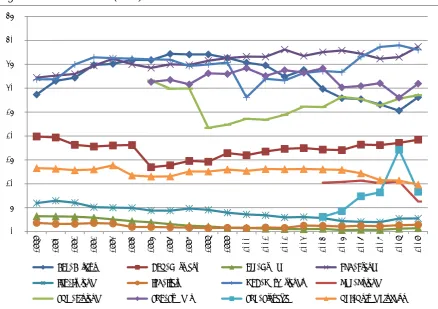
Another indication that the governments find there are difficulties for agriculture to receive credit is if the investment support of the second pillar is high. The graph in Figure 3 shows the share of investment support in total support. In the beginning of the displayed period the highest levels were in the Netherlands (about 15% in 1999 and about 11% in 2000). After that Italy has the highest percentage in 2001. Between 2002 and 2005 no country really stands out as having very high levels. In 2008 Ireland increases its share and in 2009 the highest level is in Ireland at above 20%. On the other extreme we find Sweden (zero or extremely low levels), Germany and Finland, these three countries have below average in all years. In later years also Greece and the Netherlands have had low values and UK had low levels for the most of the period.

One can discuss the efficiencies of investment support; the risks for crowding out effects are well-known, but we can still see how the agricultural or rural ministries have perceived the situation in the agricultural credit markets as being less than efficient in some countries. If not, they should not have emphasised this support over other measures.

It is particularly interesting that in Ireland, where we find no involvement from the government in the questionnaire in WP 33, the investment support for agriculture has been a big part of the support in the last couple of years. Maybe it is a way to remedy some of the effects of the financial crisis that started in 2007 and the following decrease in property values. Also Slovakia, that had no involvement according to WP33, has close to 10% in investment support levels in 2009.

In a country where credit is subsidized through investment support we can expect the LTV to be higher since the cost of loans is reduced. We would thus expect Ireland, Slovakia and maybe Belgium to have high, or at least increasing, levels of LTV in 2008 and 2009. However, of those three countries, only Belgium has a high LTV value in 2009 at 28%. Slovakia has a LTV of less than 10% and Ireland of less than 5% in 2009.

Figure 3. Investment support/ total support

Source: FADN.

5.

Conclusions

The questions to which we seek to answer are:

1) Can economic sustainability (ES) be used as a performance indicator of the financial markets? In other words, is there a connection between ES and the situation on the financial markets for the agricultural firms?

2) Is loan-to-value (LTV) lower than what the experts expected in WP 33? Does this imply that the credit levels could be higher in agriculture? Can LTV be used to measure performance of the financial markets?

To be able to answer the first question, we need to have an idea of what the financial performance is in the individual markets. Looking at the results of WP 33 there are two indications of the financial markets for agriculture being inefficient: 1) some governments are actively involved in the credit market through support measures and in some instances there are even examples of governmental credit institutes, and 2) there are very low levels in LTV ratios.

Greece, France and Belgium are the countries with the best results for the ES indicator. If our indicator would work as performance indicator we could expect that these countries have high LTV, assuming that LTV is an indicator of credit rationing. Greece, however, has very low levels of LTV, whereas France and Belgium have rather high levels of LTV. All three countries have specific government support to the agricultural credit market, and some level of investment support (Greece has very low levels).

Ireland, the Netherlands, Poland, Finland, Slovakia, Sweden and the UK all have negative results on the ES indicator in a majority of the years. Again, if the indicator would work, we might expect the countries to have low LTV – being credit rationed. But that is only partly true: Ireland, Poland, Slovakia and the UK all have rather low LTVs, whereas the Netherlands, Finland and Sweden have rather high. In this group we also find all countries

0.000 0.050 0.100 0.150 0.200 0.250

1999 2000 2001 2002 2003 2004 2005 2006 2007 2008 2009

(BEL) Belgium (DEU) Germany (ELL) Greece (FRA) France

(IRE) Ireland (ITA) Italy (NED) Netherlands (POL) Poland

with no or low levels of support to the agricultural credit market: Ireland, Sweden, Slovakia and the UK.

It is unfortunately not possible to draw any conclusions on the relation between the economic sustainability indicator and the performance of the financial institutions. The ES indicator is interesting only as a description of the economic situation of farms. The economic situation of the firm certainly plays an important role when applying for credit as we saw in WP33, but the correlation between the ES indicator and the performance of the financial institutions is not possible to determine in this study.

Regarding the second question, or set of questions, it is clear that the LTVs calculated in this WP are lower than the levels the experts expected in WP 33. This does imply that credit levels could be higher, and Curtiss (2012) sees this as an indication of credit constraints. So, if that is the case, LTV might be used as an indicator of how the financial markets perform. Regarding this indicator it is important to note that depending on who is performing the analysis, the interpretation might differ: for a commercial investor, low values are positive since the financial risk of a firm is lower if the debt-to-asset ratio is low, whereas others might see this as a sign of the firm being credit-rationed and hampered in economic and/or technical development.

References

Ciaian, P., Kancs d’A., Swinnen, J., van Herck, K., and Vranken, L. (2012), “Key Issues and Development in Farmland Sales Markets in the EU Member States and Candidate Countries”, Working Paper No 12, Factor Markets Project, CEPS, Brussels, February. Curtiss, J. (2012), “Determinants of Financial Capital Use – Review of theories and

implications for rural business”, Working Paper No. 19, Factor Markets Project, CEPS, Brussels, February.

Eurostat (2013), Farm structure statistics

(http://epp.eurostat.ec.europa.eu/portal/page/portal/eurostat/home/). FADN, (2013), Standard measures (http://ec.europa.eu/agriculture/rica/index.cfm).

Jansson, K., C.J. Huisman, C-J Lagerkvist and E. Rabinowicz (2013), “Agricultural Credit Market Institutions – A Comparison of Selected European Countries”, Working Paper No 33, Factor Markets Project, CEPS, Brussels, January.

Lagerkvist, C-J. (2001), “The source and application fund statement analysis for the proprietary firm: A revised model and an application to Swedish Agriculture 1992-1999”, paper prepared for Conference on Live Economics Issues of Agricultural Enterprises, Prague.

Nuryartono, N., M. Zeller and S. Schwarze (2005), “Credit rationing of farm household and agricultural production: Empirical evidence in the rural areas of Central Sulawesi, Indonesia”, paper presented at the Conference on International Agricultural Research for Development, Tropentag, Stuttgart-Hohenheim, 11-13 October.

Rahji, M.A.Y. and A.I. Adeoti (2010), “Determinants of agricultural credit rationing by commercial banks in South Western Nigeria”, International Research Journal of Finance and Economics, No. 37.

Swinnen J. and H. Gow (1999), “Agricultural credit problems and policies during the transition to a market economy in Central and Eastern Europe”, Food Policy, Vol. 24, No. 1, pp. 21-47.

Weber, R. and O. Musshoff (2012), “Is agricultural microcredit really more risky? Evidence from Tanzania”, Agricultural Finance Review, Vol. 72, No. 3, pp. 416-435.

Appendix 1. Stepwise calculations for all countries

(BEL) Belgium Income (incl. total subsidies) Change in assets Change in debt ES

1990 34825 7544 8574 18707

1991 32504 127 1580 30797

1992 28593 26502 15214 -13123

1993 33950 10827 4375 18748

1994 39082 25789 11479 1814

1995 36604 9295 3185 24124

1996 41990 3020 4983 33987

1997 37289 -3716 -1754 42759

1998 34906 2698 1057 31151

1999 41551 27408 7684 6459

2000 47966 4832 -1498 44632

2001 47717 2223 -1084 46578

2002 40399 21596 -914 19717

2003 49453 23466 12970 13017

2004 47196 40109 -3067 10154

2005 51743 20670 -2359 33432

2006 58697 42067 10739 5891

2007 61456 64564 11776 -14884

2008 47088 42211 3647 1230

2009 43344 -10551 13570 40325

‐20000 ‐10000 0 10000 20000 30000 40000 50000 60000 70000

1990 1992 1994 1996 1998 2000 2002 2004 2006 2008

Belgium

Change in asset

(DEU) Germany Income (incl. total subsidies) Change in assets Change in debt ES

1990 12710 -5082 -1616 19408

1991 13057 13576 -1942 1423

1992 11332 20377 2551 -11596

1993 14081 1863 1080 11138

1994 18187 19150 3744 -4707

1995 21408 259063 19070 -256725

1996 23143 -13221 591 35773

1997 23614 -25301 1603 47312

1998 20108 17819 1646 643

1999 27798 74675 22694 -69571

2000 30827 333 -2780 33274

2001 29359 10011 6746 12602

2002 21704 12131 5771 3802

2003 22576 10187 2873 9516

2004 32183 24973 2115 5095

2005 32255 5879 271 26105

2006 37308 33888 14426 -11006

2007 48144 12092 1394 34658

2008 31079 14095 6144 10840

2009 25082 3392 5841 15849

‐50000 0 50000 100000 150000 200000 250000 300000

1990 1992 1994 1996 1998 2000 2002 2004 2006 2008

Germany

Change in asset

(ELL) Greece Income (incl. total subsidies) Change in assets Change in debt ES

1990 7536 -208 -25 7769

1991 8888 -624 -56 9568

1992 7643 1752 -53 5944

1993 8085 -504 -224 8813

1994 9022 1372 -172 7822

1995 9465 1250 -112 8327

1996 9061 4249 -164 4976

1997 8913 1896 -173 7190

1998 9196 -2548 -128 11872

1999 8852 1351 -154 7655

2000 9645 -1098 -1 10744

2001 9425 3247 -118 6296

2002 11249 545 -38 10742

2003 10687 2299 -6 8394

2004 10892 4243 67 6582

2005 12341 2317 -174 10198

2006 11814 3235 55 8524

2007 12599 621 -14 11992

2008 11858 -429 197 12090

2009 10673 3484 108 7081

‐3000 ‐2000 ‐1000 0 1000 2000 3000 4000 5000

1990 1992 1994 1996 1998 2000 2002 2004 2006 2008

Greece

Change in asset

(FRA) France Income (incl. total subsidies) Change in assets Change in debt ES

1990 23176 6507 2957 13712

1991 21666 -2457 -126 24249

1992 22214 11766 7546 2902

1993 20995 -7594 250 28339

1994 27124 15831 3206 8087

1995 29678 13246 2915 13517

1996 30997 12925 6240 11832

1997 29822 5024 1411 23387

1998 31046 6477 4516 20053

1999 31166 19907 8665 2594

2000 29334 7313 3511 18510

2001 28354 -3000 -1209 32563

2002 29903 14113 9602 6188

2003 28437 5766 -1794 24465

2004 29086 20094 9949 -957

2005 28037 -618 860 27795

2006 31637 16051 3783 11803

2007 40602 13124 1266 26212

2008 31830 19414 8304 4112

2009 16408 -13527 2684 27251

‐20000 ‐15000 ‐10000 ‐5000 0 5000 10000 15000 20000 25000

1990 1992 1994 1996 1998 2000 2002 2004 2006 2008

France

Change in asset

(IRE) Ireland Income (incl. total subsidies) Change in assets Change in debt ES

1990 9655 -1338 971 10022

1991 9063 -785 -913 10761

1992 11647 7897 -1530 5280

1993 12324 -5341 -478 18143

1994 13638 16008 659 -3029

1995 13312 14930 -572 -1046

1996 13325 21846 897 -9418

1997 14958 25874 2457 -13373

1998 11816 17548 -50 -5682

1999 11901 39900 -197 -27802

2000 14089 65665 1121 -52697

2001 15140 24721 101 -9682

2002 15417 76060 306 -60949

2003 16294 -23019 -243 39556

2004 16847 56189 462 -39804

2005 18028 183210 548 -165730

2006 18860 184093 2824 -168057

2007 21633 89330 1054 -68751

2008 18866 -62194 5845 75215

2009 13573 -85525 -2063 101161

‐100000 ‐50000 0 50000 100000 150000 200000

1990 1992 1994 1996 1998 2000 2002 2004 2006 2008

Ireland

Change in asset

(ITA) Italy Income (incl. total subsidies) Change in assets Change in debt ES

1990 10737 6475 -155 4417

1991 11933 11369 207 357

1992 10136 2911 285 6940

1993 9195 -14399 -393 23987

1994 11112 88798 -52 -77634

1995 13401 -6554 -84 20039

1996 13717 25952 113 -12348

1997 14012 9534 -102 4580

1998 13716 47849 130 -34263

1999 14940 8323 280 6337

2000 13878 -5508 -358 19744

2001 15291 -1549 477 16363

2002 20625 104223 597 -84195

2003 22240 -95869 663 117446

2004 21804 -19350 -355 41509

2005 22631 46175 113 -23657

2006 23606 10879 631 12096

2007 27459 5081 -247 22625

2008 27227 -19408 435 46200

2009 24961 -2909 249 27621

‐150000 ‐100000 ‐50000 0 50000 100000 150000

1990 1992 1994 1996 1998 2000 2002 2004 2006 2008

Italy

Change in asset

(NED) Netherlands Income (incl. total subsidies) Change in assets Change in debt ES

1990 38545 9350 3036 26159

1991 37324 5415 18267 13642

1992 26684 31343 19376 -24035

1993 24508 51784 17792 -45068

1994 38463 49901 17471 -28909

1995 36085 29316 9499 -2730

1996 33252 4089 979 28184

1997 41692 36877 3595 1220

1998 25511 57316 22421 -54226

1999 22869 132419 49884 -159434

2000 41655 251659 3369 -213373

2001 46517 184220 104441 -242144

2002 33840 62339 15112 -43611

2003 42617 2341 22872 17404

2004 36152 70084 29562 -63494

2005 46220 106679 31948 -92407

2006 55096 12369 55714 -12987

2007 49539 89156 67996 -107613

2008 32489 87958 40242 -95711

2009 19153 153291 41238 -175376

0 50000 100000 150000 200000 250000 300000

1990 1991 1992 1993 1994 1995 1996 1997 1998 1999 2000 2001 2002 2003 2004 2005 2006 2007 2008 2009

Netherlands

Change in asset

(POL) Poland Income (incl. total subsidies) Change in assets Change in debt ES

2005 6494 3649 491 2354

2006 8211 5213 746 2252

2007 10351 11644 794 -2087

2008 8155 11562 1518 -4925

2009 7005 34109 -1974 -25130

‐5000 0 5000 10000 15000 20000 25000 30000 35000 40000

2005 2006 2007 2008 2009

Poland

Change in asset

(SUO) Finland Income (incl. total subsidies) Change in assets Change in debt ES

1996 22207 4402 -1241 19046

1997 19958 1624 539 17795

1998 16278 55039 -999 -37762

1999 18379 27696 7603 -16920

2000 22625 7263 4646 10716

2001 23204 7708 1332 14164

2002 24228 -90 2600 21718

2003 22324 10125 7010 5189

2004 20306 17784 4413 -1891

2005 19764 25038 12980 -18254

2006 18114 23473 5184 -10543

2007 27651 30717 3749 -6815

2008 20247 15280 9253 -4286

2009 17174 3467 3848 9859

‐10000 0 10000 20000 30000 40000 50000 60000

1996 1997 1998 1999 2000 2001 2002 2003 2004 2005 2006 2007 2008 2009

Finland

Change in asset

(SVE) Sweden Income (incl. total subsidies) Change in assets Change in debt ES

1996 1582 10898 4732 -14048

1997 5867 -9936 -6067 21870

1998 -1747 1618 7682 -11047

1999 2183 16965 5180 -19962

2000 5891 54616 22693 -71418

2001 7024 -3160 -7295 17479

2002 6995 60209 24917 -78131

2003 6335 15380 2827 -11872

2004 6574 25606 12733 -31765

2005 11331 104769 12577 -106015

2006 10708 58761 19597 -67650

2007 29479 -3779 2546 30712

2008 29684 37626 -8876 934

2009 6243 -63510 355 69398

‐80000 ‐60000 ‐40000 ‐20000 0 20000 40000 60000 80000 100000 120000

1996 1997 1998 1999 2000 2001 2002 2003 2004 2005 2006 2007 2008 2009

Sweden

Change in asset

(SVK) Slovakia Income (incl. total subsidies) Change in assets Change in debt ES

2005 1032 40897 18426 -58291

2006 -90062 -422703 13180 319461

2007 12288 242126 28143 -257981

2008 -6569 -453635 34112 412954

2009 -123377 1135724 24611 -1283712

‐600000 ‐400000 ‐200000 0 200000 400000 600000 800000 1000000 1200000 1400000

2005 2006 2007 2008 2009

Slovakia

Change in asset

(UKI) United Kingdom Income (incl. total subsidies) Change in assets Change in debt ES

1990 20882 -7308 -1590 29780

1991 21526 -6529 -2491 30546

1992 23602 -49509 -5614 78725

1993 30008 2370 4584 23054

1994 35667 60287 -3409 -21211

1995 42703 22801 1323 18579

1996 39118 38296 4612 -3790

1997 27232 146092 24810 -143670

1998 19553 -6234 -962 26749

1999 19564 43110 8786 -32332

2000 22098 39310 2683 -19895

2001 28068 114817 18398 -105147

2002 34881 -2268 -815 37964

2003 41015 -55461 -6757 103233

2004 30002 30707 3212 -3917

2005 35896 128615 15777 -108496

2006 38928 109402 5732 -76206

2007 55343 196818 4810 -146285

2008 49285 -95078 -11548 155911

2009 42050 55337 -5328 -7959

‐150000 ‐100000 ‐50000 0 50000 100000 150000 200000 250000

1990 1991 1992 1993 1994 1995 1996 1997 1998 1999 2000 2001 2002 2003 2004 2005 2006 2007 2008 2009

UK

Change in asset

The Factor Markets project in a nutshell

Title Comparative Analysis of Factor Markets for Agriculture across the Member States

Funding scheme Collaborative Project (CP) / Small or medium scale focused research project

Coordinator CEPS, Prof. Johan F.M. Swinnen

Duration 01/09/2010 – 31/08/2013 (36 months)

Short description Well functioning factor markets are a crucial condition for the competitiveness and growth of agriculture and for rural development. At the same time, the functioning of the factor markets themselves are influenced by changes in agriculture and the rural economy, and in EU policies. Member state regulations and institutions affecting land, labour, and capital markets may cause important heterogeneity in the factor markets, which may have important effects on the functioning of the factor markets and on the interactions between factor markets and EU policies.

The general objective of the FACTOR MARKETS project is to analyse the functioning of factor markets for agriculture in the EU-27, including the Candidate Countries. The FACTOR MARKETS project will compare the different markets, their institutional framework and their impact on agricultural development and structural change, as well as their impact on rural economies, for the Member States, Candidate Countries and the EU as a whole. The FACTOR MARKETS project will focus on capital, labour and land markets. The results of this study will contribute to a better understanding of the fundamental economic factors affecting EU agriculture, thus allowing better targeting of policies to improve the competitiveness of the sector.

Contact e-mail [email protected]

Website www.factormarkets.eu

Partners 17 (13 countries)

EU funding 1,979,023 €

EC Scientific officer Dr. Hans-Jörg Lutzeyer

Comparative Analysis of Factor Markets

for Agriculture across the Member States