Development and application of statistical and quantum mechanical methods for modelling molecular ensembles

statistical and quantum mechanical

methods for modelling molecular

ensembles

By

Ellen T. Swann

A thesis submitted for the degree of Doctor of Philosophy of the Australian National University

Research School of Chemistry

February, 2018

This thesis is an account of research undertaken between February 2014 and June 2017 as part of a collaboration between CSIRO and ANU.

Except where acknowledged in the customary manner, the material presented in this thesis is, to the best of my knowledge, original and has not been submitted in whole or part for a degree in any university. This research is supported by an Australian Government Research Training Program (RTP) Scholarship.

Ellen T. Swann February, 2018

First and foremost I would like to thank my amazing supervisors Michelle Coote, Amanda Barnard and Manolo Per. Your support and guidance over the last three and a half years has been greatly appreciated. This thesis and PhD would not have been possible without you.

I would also like to thank past and present VNLab members, for all they have taught me. Thank you especially to Deidre, for her help with all things QMC related and teaching me SQL and Michael, for teaching me archetypal analysis.

Finally, a massive thank you to Mum, Dad, Hillary, Hugh and Ned for their unwavering love and support. I’d also like to thank my family and friends, for everything they’ve done to help me get through the last 8 years of study. Lastly, thank you to Han, for keeping me sane despite the puns.

The development of new quantum chemical methods requires extensive benchmarking to establish the accuracy and limitations of a method. Current benchmarking practices in computational chemistry use test sets that are subject to human biases and as such can be fundamentally flawed. This work presents a thorough benchmark of diffusion Monte Carlo (DMC) for a range of systems and properties as well as a novel method for developing new, unbiased test sets using multivariate statistical techniques. Firstly, the hydrogen abstraction of methanol is used as a test system to develop a more efficient protocol that minimises the computational cost of DMC without compromising accuracy. This protocol is then applied to three test sets of reaction energies, including 43 radical stabilisation energies, 14 Diels-Alder reactions and 76 barrier heights of hydrogen and non-hydrogen transfer reactions. The average mean absolute error for all three databases is just 0.9 kcal/mol.

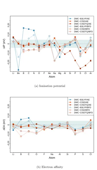
The accuracy of the explicitly correlated trial wavefunction used in DMC is demon-strated using the ionisation potentials and electron affinities of first- and second-row atoms. A determinant trial wavefunction reduces the errors for systems with strong multi-configuration character, as well as for predominantly single-reference systems. It is shown that the use of pseudopotentials in place of all-electron basis sets slightly increases the error for these systems. DMC is then tested with a set of eighteen challenging reactions. Incorporating more determinants in the trial wavefunction reduced the errors for most sys-tems but results are highly dependent on the active space used in the CISD wavefunction. The accuracy of multi-determinant DMC for strongly multi-reference systems is tested for the isomerisation of diazene. In this case no method was capable of reducing the error of the strongly-correlated rotational transition state.

Finally, an improved method for selecting test sets is presented using multivariate statistical techniques. Bias-free test sets are constructed by selecting archetypes and pro-totypes based on numerical representations of molecules. Descriptors based on the one-, two- and three-dimensional structures of a molecule are tested. These new test sets are then used to benchmark a number of methods.

Declaration ii

Acknowledgements iii

Abstract iv

List of Figures viii

List of Tables 1

1 Introduction 2

1.1 List of publications . . . 5

1.2 References . . . 5

2 Theoretical Methods 6 2.1 Introduction . . . 6

2.2 Ab initio methods . . . 7

2.2.1 Post-HF methods . . . 8

2.2.2 Coupled-cluster theory . . . 9

2.2.3 Multi-reference methods . . . 10

2.2.4 Composite high-level methods . . . 10

2.3 Density functional theory . . . 11

2.4 Quantum Monte Carlo . . . 12

2.4.1 Trial wavefunction . . . 12

2.4.2 Variational Monte Carlo (VMC) . . . 13

2.4.3 Diffusion Monte Carlo (DMC) . . . 14

2.4.4 Multi-determinant DMC . . . 17

2.5 Basis sets . . . 17

2.5.1 Pseudopotentials . . . 18

2.6 Summary . . . 19

2.7 References . . . 20

3 An efficient protocol for diffusion Monte Carlo calculations 25 3.1 Introduction . . . 25

3.2 Trial wavefunction . . . 26

3.3 Computational details . . . 28

3.4 Results and discussion . . . 29

3.4.1 Approximations . . . 31

3.4.2 Accuracy . . . 32

3.4.3 Cost . . . 32

3.4.4 Variance . . . 34

3.4.5 Time-step error . . . 35

3.5 Summary . . . 36

3.6 References . . . 37

4 Calculating barrier heights with quantum Monte Carlo 40 4.1 Introduction . . . 40

4.2 Methods . . . 41

4.3 Radical stabilisation energy . . . 41

4.4 Diels-Alder reactions . . . 44

4.5 Hydrogen and non-hydrogen transfer barrier heights . . . 46

4.6 Comparison to other methods . . . 51

4.7 Summary . . . 51

4.8 References . . . 52

5 Ionisation potentials and electron affinities of first- and second-row atoms 56 5.1 Introduction . . . 56

5.2 Methods . . . 58

5.3 Single-determinant DMC . . . 58

5.4 Multi-determinant DMC . . . 61

5.5 BFD pseudopotential . . . 65

5.6 Summary . . . 67

5.7 References . . . 67

6 Difficult reactions 70 6.1 Introduction . . . 70

6.2 Method . . . 71

6.3 Single-determinant DMC . . . 73

6.4 Multi-determinant DMC . . . 73

6.4.1 Active space selection . . . 73

6.4.2 Non-hydrogen hypervalent compounds . . . 74

6.4.3 Atomisation energies of large molecules . . . 76

6.4.4 Isomerisation energies of organic molecules . . . 77

6.4.5 Binding energy of sulphur . . . 79

6.5 Comparison to other methods . . . 79

6.6 Summary . . . 81

7 The isomerization of diazene (N₂H₂) 85

7.1 Introduction . . . 85

7.2 Methodology . . . 87

7.3 Single-determinant DMC . . . 87

7.4 Multi-determinant DMC . . . 88

7.4.1 Total energies . . . 88

7.4.2 Relative energies . . . 94

7.5 Future work . . . 95

7.6 Summary . . . 99

7.7 References . . . 99

8 Bias-free chemical test sets 102 8.1 Introduction . . . 102

8.1.1 Multivariate statistical techniques . . . 104

8.1.2 Descriptors . . . 107

8.2 Computational methods . . . 109

8.2.1 Data set . . . 109

8.2.2 Descriptors . . . 109

8.2.3 Machine learning . . . 109

8.2.4 Atomisation energies . . . 111

8.3 Results and discussion . . . 112

8.3.1 Principal component analysis . . . 112

8.3.2 K-means clustering . . . 113

8.3.3 Archetypal analysis . . . 115

8.3.4 New test sets . . . 115

8.3.5 Organic molecules . . . 118

8.3.6 Machine learning . . . 119

8.3.7 Atomisation energies . . . 119

8.4 Summary . . . 124

8.5 References . . . 124

2.1 Examples of the excited determinants used in a configuration interaction

wavefunction . . . 9

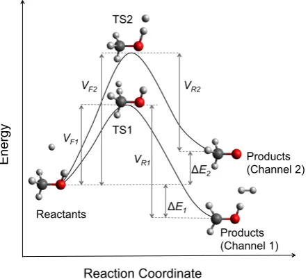
3.1 The potential energy surface for the reaction between atomic hydrogen and methanol. . . 26

3.2 The errors of DMC barrier heights for the hydrogen abstraction of methanol 33 3.3 DMC timings for methanol (CH3OH) relative to original pseudopotential settings . . . 34

3.4 VMC variance of the local energy for CH₃OH using different settings for the Jastrow factor and pseudopotentials. . . 35

3.5 DMC energies as a function of imaginary time-step for the TS2 geometry, using the BFD pseudopotentials. . . 36

4.1 The Diels-Alder test set (DARC) . . . 44

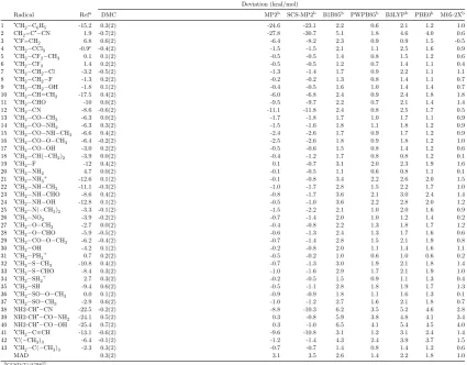
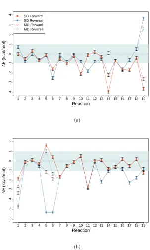
4.2 The errors in DMC barrier heights for the BH76 test set . . . 47

4.3 The errors in DMC barrier heights using different energy-based determinant truncation schemes for four reactions from BH76 . . . 49

4.4 Comparison of the MAD for RSE43, DARC and BH76 test sets for DMC, ab initio wavefunction and DFT methods . . . 51

5.1 The errors in DMC ionisation potentials (a) and electron affinities (b) for first- and second-row atoms . . . 60

5.2 DMC nodal correlation energy as a fraction of the total DMC-B3LYP energy for CISD and CISDTQ trial wavefunctions . . . 63

5.3 Comparison of DMC-CISD ionisation potentials . . . 64

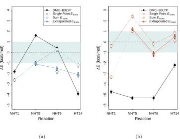
6.1 The errors in DMC reaction energies for the DC18 test set . . . 72

6.2 The isomerisation reactions in DC18 . . . 78

6.3 Comparison of the MAD for the DC18 test set for DMC, ab initio wave-function and DFT methods . . . 80

7.1 Diazene isomers and transition states . . . 86

7.2 Total energies, E (Ha), of the diazene isomers and transition states as a function of the number of orbitals, Norb, in the active space (Ne, Norb). . . 91

7.3 Total DMC energies, E (Ha), of the diazene isomers and transition states as a function of the number of orbitals, Norb, in the active space (Ne, Norb). 92

7.4 Nodal correlation energy recovered by CISD and CISDTQ trial wavefunc-tions in DMC calculawavefunc-tions . . . 93 7.5 The errors of DMC relative energies of diazene isomers . . . 96 7.6 Mean absolute deviations (MAD) of the DMC relative energies of diazene

isomers . . . 97

8.1 Explained variance as a function of the number of components for different multivariate statistical methods . . . 112 8.2 Hierarchical clustering dendrograms of the cluster prototypes . . . 114 8.3 Simplex plots of the topological and Coulomb matrix descriptors . . . 116 8.4 Histogram of the errors for the entire data set and new test sets based on

topological or Coulomb matrix descriptors . . . 117 8.5 Explained variance as a function of the number of components for different

multivariate statistical methods for an organic set of molecules . . . 118 8.6 Hierarchical clustering dendrograms of the cluster prototypes for a set of

organic molecules . . . 120 8.7 Simplex plot of the TOPO archetypes for an organic set of molecules . . . . 121 8.8 Histogram of the errors for an organic set of molecules and new test sets

based on topological or Coulomb matrix descriptors . . . 122 8.9 Scatter plot of ∆E predictions for machine learning models using test sets

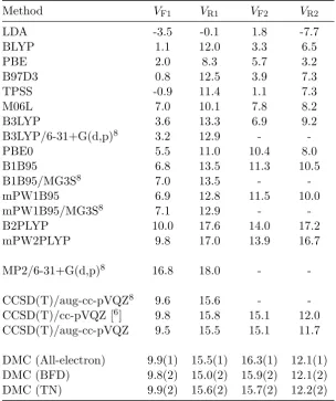
3.1 Reaction barrier heights for the H abstraction of methanol by an H atom (in kcal/mol) using different methods . . . 30

4.1 Summary of results for the radical stabilisation energies test set (RSE43) . 43 4.2 Summary of results for the Diels-Alder test set (DARC) . . . 45 4.3 The 38 hydrogen-transfer (HTBH) and 38 non-hydrogen transfer (NHTBH)

barrier heights in the BH76 test set. . . 46 4.4 Summary of the final number of CSFs used in the DMC calculation of each

molecule for different Etrunc values. . . 50

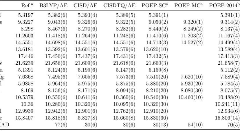
5.1 DMC ionisation potentials for first- and second-row atoms using all-electron basis sets. . . 59 5.2 DMC electron affinities for first- and second-row atoms using all-electron

basis sets. . . 59 5.3 Mean absolute deviation of DMC results for ionisation potentials and

elec-tron affinities of first- and second-row atoms . . . 65

6.1 The difficult cases (DC18) test set . . . 71 6.2 Details of the active spaces, CSFs and Dets used in multi-determinant trial

wavefunctions . . . 75

7.1 Relative energies of diazene isomers and transition states with respect to

trans-N2H2 . . . 88 7.2 Summary of total energies and details of multi-determinant wavefunctions

used in DMC calculations for the isomers and transition states of diazene. . 89 7.3 DMC relative energies of diazene isomers and transition states with respect

totrans-N2H2 . . . 94

8.1 Two-dimensional topological descriptors . . . 110 8.2 Details of the optimum regression models of ∆E . . . 121 8.3 Mean absolute deviation of DMC results for atomisation energies of the

molecules in the CMolsC-1 and CMolsT-1 test sets. . . 123

Introduction

Quantum chemical methods have become an integral part of the chemistry field over the last 50 years. Advances in drug discovery1, 2 _{and high-throughput material screening}3 would not have been possible without them but their impact is much broader. They allow hypothetical and unobserved systems to be studied in great detail. The foundation of all computational chemistry methods lies in solving the time-independent Schr¨odinger wave equation (SWE),

ˆ

HΨ =EΨ (1.1)

where ˆH is the electronic Hamiltonian operator, Ψ is the wavefunction solution andE is the electronic energy of the system of interest. If the Hamiltonian and wavefunction are known then virtually any property can be calculated. The correlated nature of sub-atomic interactions means the Schr¨odinger equation can only be solved exactly for systems with one or two electrons. Approximations must be made to solve it for larger systems. Tradi-tional electronic structure methods like Hartree Fock (HF) theory and density funcTradi-tional theory (DFT) are well established and chemically accurate results have been obtained for a range of systems.4–7 _{Unfortunately this accuracy comes with a large cost. Post-HF} CCSD(T) scales as N7 _{with respect to system size, N. DFT methods are more affordable} but their performance is unreliable; accurate DFT results for small systems don’t neces-sarily translate for large systems.8 _{A promising alternative to these methods is quantum} Monte Carlo (QMC).

QMC uses stochastic integration and has greater freedom in the form of the trial wavefunction compared to ab initio wavefunction theory (WFT) or DFT methods. The commonly-used Slater-Jastrow trial wavefunction explicitly accounts for the static and dynamic correlation in a system. By using statistical sampling QMC methods are intrinsi-cally parallelisable and scale nearly perfectly with the number of available cores. They are ideally positioned to take full advantage of the new wave of parallel computers compared to more traditional methods.

The development of new quantum chemical methods requires extensive benchmarking to demonstrate robustness and identify potential weaknesses and shortcomings. Perfor-mance of a method is measured by the error, defined as the difference between the calcu-lated value and some reference value that has been obtained from experiment or high-level

electronic structure methods. Commonly used metrics include the mean unsigned error (MUE) or mean absolute deviation (MAD) but other metrics like root mean squared error (RMSE) can be used. Smaller errors are desirable and chemical accuracy is defined as an error of 1 kcal/mol or less. For properties where energy differences are expected to be small, like the relative energies of conformers, this accuracy needs to be on the order of 0.1-0.2 kcal/mol. The outcomes of benchmarking guide users towards the most appropri-ate method for a specific problem and identify the types of systems where a method might fail. Computational chemistry is increasingly being used for simulations where experiment is impossible and it is essential that we can estimate the accuracy of the calculations in these situations.

Benchmarking is a powerful tool for assessing and comparing the accuracy of electronic structure methods but there are serious limitations to the current methodology. The standard practice in computational chemistry is to benchmark using test sets. There are now hundreds, if not thousands, of these sets available in the literature for a vast range of properties. These test sets have been built using ‘chemical intuition’ and are biased by how we perceive chemical space. This has led to redundancies in test sets and benchmarking results that are highly dependent on the systems studied. Not using a comprehensive test set to evaluate a method can lead to biases in reported error when one class of reaction is over represented.9–12 _{The standard practice has become a cumbersome} process requiring thousands of calculations to overcome these challenges. Some effort has been directed at finding small, representative subsets but this is limited to only a few test sets for a handful of properties.13 _{It also requires thousands of data points from previous} benchmarking studies with the biased test sets.

An alternative method for building these test sets is to use multivariate statistics and remove the human bias entirely. Chemical space can be represented by numerical descrip-tors based on the structure or physical properties of molecules. Techniques like k-means clustering and archetypal analysis are routinely used in other fields to find combinations of points that best represent or summarise large data sets. By developing these techniques for computational chemistry, smaller databases can be created for benchmarking that are designed to provide critical tests of methods without redundancy.

1.1

List of publications

1. Swann, E.T., Coote, M.L., Barnard, A.S., Per, M.C., ‘Efficient protocol for quan-tum Monte Carlo calculations of hydrogen abstraction barriers : Application to methanol‘, Int. J. Quantum Chem,2017,117, 1- 7. (Appendix 1)

2. Swann, E.T., Fernandez, M., Coote, M.L., Barnard, A.S., ‘Bias-free chemically di-verse test sets from machine learning’, submitted

1.2

References

1_{W. L. Jorgensen, Science 2004,303, 1813–1818.} 2_{W. L. Jorgensen, Acc. Chem. Res.2009,42, 724–733.}

3_{S. Curtarolo, G. L. Hart, M. B. Nardelli, N. Mingo, S. Sanvito, O. Levy, Nat. Mater.}

2013,12, 191–201.

4_{S. M. Bachrach, Computational Organic Chemistry, John Wiley & Sons Inc., 2014.} 5_{F. Jensen, Introduction to Computational Chemistry 2nd ed., Wiley,2007.}

6_{C. J. Cramer, Essentials of Computational Chemistry: Theories and Models 2nd ed.,}

John Wiley & Sons Inc., 2004.

7_{E. G. Lewars, Computational Chemistry. Introduction to the Theory and Applications}

of Molecular and Quantum Mechanics, Kluwer Academic Publishers, 2003. 8_{A. J. Cohen, P. Mori-S´anchez, W. Yang, Chem. Rev.2012,112, 289–320.} 9_{J. J. P. Stewart, J. Comput. Chem. 1989,10, 155–164.}

10_{J. J. P. Stewart, J. Comput. Chem. 1989,10, 209–220.}

11_{G. I. Csonka, A. Ruzsinszky, J. Tao, J. P. Perdew,Int. J. Quantum. Chem. 2005,101,} 506–511.

12_{S. Grimme, J. Phys. Chem. A. 2005,109, 3067–3077.}

Theoretical Methods

2.1

Introduction

The Schr¨odinger wave equation:1

ˆ

HΨ =EΨ (2.1)

describes the total energy (E) of a system as a function of the Hamiltonian ( ˆH) operating on the wavefunction (Ψ). If the Hamiltonian and wavefunction are known then virtually any physical or chemical property of a given molecular system can be calculated. The Hamiltonian is an operator describing the observable energy of the system and can be written in terms of kinetic ( ˆT) and potential ( ˆV) energy operators for electrons (e) and nuclei (n):

ˆ

H= ˆTn+ ˆTe+ ˆVee+ ˆVne+ ˆVnn (2.2)

This definition ignores relativistic effects but provides a good description for the relatively light first- and second-row atoms.2 _{The Born-Oppenheimer approximation}3 _{is commonly} used to simplify wavefunction solutions to the Schr¨odinger wave equation by decoupling the motion of electrons and nuclei. It assumes the nuclei are infinitely heavy relative to the electrons and the electrons move instantaneously in response to the nuclei. The electronic Hamiltonian, ˆHelec, can then be written as:

ˆ

Helec = ˆTe+ ˆVee+ ˆVne+ ˆVnn

=−1 2

n X

i ∇2_i +

n X

i<j 1 rij

− N X

I n X

i ZI rIi

+ ˆVnn

(2.3)

for a system of n electrons and N nuclei, where rij is the distance between electrons

i and j and ZI is the atomic number of nuclei I. The Born-Oppenheimer approximation reduces the Schr¨odinger wave equation to an electronic problem and wavefunction solutions describe the motion ofn electrons moving in a field ofN fixed nuclei. Electronic structure theory is primarily concerned with finding the electronic wavefunction solutions and their corresponding energy.

The Schr¨odinger wave equation is a second-order linear differential equation and exact solutions exist for only a small number of systems. Electronic structure methods use

different approximations in a trade off between accuracy and computational cost. Hartree-Fock (HF) theory uses the mean-field approximation but fails to account for electron correlation and post-HF ab initio wavefunction theory (WFT) attempts to recover this correlation energy. Density functional theory (DFT) reduces the dimensionality of the problem by using the electron density in place of the wavefunction. Quantum Monte Carlo (QMC) methods use stochastic integration and have much greater freedom in the form of the trial wavefunction. An overview of each method is provided below. More detailed information forab initioand DFT methods can be found in Refs. 2,4–6. Detailed information for QMC methods can be found in Refs. 7–10.

2.2

Ab initio

methods

Hartree-Fock (HF) theory11 _{is the foundation of ab initio wavefunction methods. It} ap-proximates an exact N-body wavefunction by using single particle functions (orbitals) to describe the distribution of each electron. The non-relativistic electronic Hamiltonian in Equation 2.3 depends only on the spatial coordinates, ri, of each electron but electrons are also characterised by a spin quantum number. The coordinate xi= (ri, σi) is used in-stead to define the spin and three spatial coordinates of an electroni. The Pauli exclusion principle states that no two electrons can occupy the same point in configuration space12 and wavefunction solutions to Equation 2.3 must be antisymmetric with respect to the interchange of any two electrons, such that for a system of N electrons:

Ψ(x1, ...,xm, ...,xn, ...,xN) =−Ψ(x1, ...,xn, ...,xm, ...,xN) (2.4) The HF wavefunction is given by a singleN-electron Slater determinant:13

ΨHF=|ψ1, ψ2, ...ψNi= 1 √

N!

ψ1(x1) ψ2(x1) ... ψN(x1) ψ1(x1) ψ2(x1) ... ψN(x1)

..

. ... . .. ...

ψ1(xN) ψ2(xN) ... ψN(xN)

(2.5)

The set of functionsψiare the individual one-electron wavefunctions, also called molec-ular orbitals (MOs), that describe the distribution of an electron as a function of its spin and spatial coordinatesx. Interchanging any two electrons in the Slater-determinant will change the sign of ΨHF, satisfying the antisymmetry requirement. The expectation value of the energy is given byE =hΨ|Hˆ|Ψi if Ψ is normalised. For the HF wavefunction:

EHF= X

i Hi+

1 2

X

ij

(Jij−Kij) (2.6)

the electrons and Kij is a two-electron term associated with the exchange of electronic coordinates. The variational theorem states that the energy determined by an approximate wavefunction will always be equal to or greater than the energy of the exact wavefunction. The coefficients of the MOs are optimised to minimiseEHF in a process that is carried out iteratively and is known as theSelf-Consistent Field (SCF) method.11, 14–18

There are several variations of HF theory. Restricted Hartree-Fock (RHF) assumes the spin-up (α) and spin-down (β) electrons of an electron pair are energetically degenerate and assigns them to the same spatial MO. This is a reasonable assumption for closed shell species but open shell systems like radicals have uneven numbers ofαandβelectrons. Un-restricted Hartree-Fock (UHF) method allows separate sets of MOs forα and β electrons but this can result in spin-contamination and the wavefunctions are no longer eigenfunc-tions of ˆS2_.19 _{Restricted open-shell Hartree-Fock (ROHF) pairs α and β electrons in a} similar manner to RHF but allocates separate MOs for unpaired electrons.6

The orbitals used in HF theory are independent of the instantaneous motion of other electrons and introduce an intrinsic error known as the ‘correlation error’. The correlation energy is defined as:

Ecorr=Eexact−EHF (2.7)

The HF energy provides an upper limit on the electronic energy of a system and the correlation energy will always be negative. The correlation error increases with system size and the number of electrons. It accounts for only a small percentage of the total electronic energy of a system but is important when energy differences are considered and post-HF methods are chiefly concerned with recovering this energy. Correlation energy is often characterised as either static or dynamic. Static correlation arises from near-degeneracy effects and is important in systems where different orbitals have similar energies such as stretched bonds and low-lying excited states. Dynamic correlation arises from the instantaneous electron-electron interactions. For systems where dynamic correlation is dominant a single determinant is sufficient and HF provides a reasonable description. For systems with significant static correlation more than one reference determinant should be used.

2.2.1 Post-HF methods

Configuration interaction

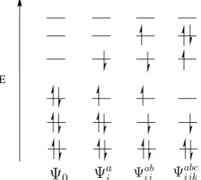
The configuration interaction (CI) method allows excitations from occupied orbitals into one or more unoccupied ‘virtual’ orbitals.20 _{Single excitations (Ψ}a

i) promote one electron from an occupied orbital, i, into a virtual orbital, a. Double excitations promote two electrons and so forth. Examples of some of these excitations are shown in Figure 2.1. These different configurations are then mixed together to give a better approximation of the true wavefunction:

ΨCI=c0Ψ0+ X

i ca

iΨai + X

ij cab

ijΨabij + X

ijk cabc

Ψa_i Ψab ij E

Ψ0 Ψabcijk

Figure 2.1: Examples of the types of excitations used to generate a configuration interaction wavefunction. Excitations shown include single (Ψa

i), double (Ψabij) and triple (Ψabc

ijk) excitations from the Hartree-Fock reference, Ψ0.

where i, j, k, ... refer to occupied orbitals and a, b, c, ... refer to unoccupied (vir-tual) levels. The coefficients, ca

i, cabij, cabcijk, ..., are found using the variational theorem. Configuration state functions (CSFs) are symmetry-adapted linear combinations of Slater determinants and are often used in place of determinants to reduce the number of func-tions.

Full configuration interaction (FCI) includes all possible configurations for a system with N electrons (up to N-fold excitations) and is exact within a given set of basis func-tions. The cost of FCI increases exponentially and in practice the CI expansion is trun-cated according to excitation level.21 _{In this work CISD (single and double excitations)} and CISDTQ (single, double, triple and quadruple excitations) were used. Truncated CI methods are variational but no longer size consistent i.e. the energy of a system with

N non-interacting particles is not equal to the sum of the energy of N isolated systems. They recover smaller fractions of the correlation energy as system size increases and can be unreliable for dissociation energies and other energy differences, particularly for larger molecules.22

2.2.2 Coupled-cluster theory

Coupled-cluster (CC) theory23–26 _{defines the true wavefunction as:}

ΨCC=e ˆ T_Ψ

HF (2.9)

where ˆT is an excitation operator and can be written as a linear combination of excitations, up to N-fold excitations for system withN electrons:

ˆ

T = ˆT1+ ˆT2+ ˆT3+...+ ˆTN (2.10)

truncated CC is no longer variational. Coupled cluster with single, double and perturba-tive triple excitations (CCSD(T)27_{) has become the gold-standard in quantum chemical} methods and is expected to give results close to the FCI limit for a given basis set. The basis set error is often removed by extrapolating to the complete basis set limit.2

2.2.3 Multi-reference methods

The methods described above use a single Slater determinant as the reference function. This approach fails for systems where static correlation is important and more than one configuration contributes significantly to the ground state energy. The multi-configuration self consistent field (MCSCF) method begins with linear combination of Slater determi-nants. It is similar in principle to CI but optimises the MOs used for constructing the determinants as well as the determinant coefficients in an iterative SCF procedure. The Slater determinants included are selected a priori, commonly using the complete active space (CAS) method.28 _{The CAS wavefunction includes all possible excitations within a} set of active orbitals. The near-degeneracies that result in static correlation most often affect the highest occupied and lowest unoccupied orbitals and the active space is usu-ally built using a certain number of these orbitals. The general notation is CAS(n, m), referring ton electrons distributed amongst m active orbitals.

The CASSCF wavefunction does not include dynamic correlation but this can be incor-porated with multi-reference configuration interaction (MRCI).28 _{MRCI is similar to CI} as described above but generates all possible excitations for each determinant in a multi-reference wavefunction. Each determinant is treated equivalently. A cheaper alternative is complete active space second order perturbation theory (CASPT2), where perturbative corrections are made to the CASSCF expansion based on the single and double excitations from every determinant in the active space.29 _{Including the perturbations destroys the} variationality of MCSCF.

2.2.4 Composite high-level methods

Composite methods attempt to reproduce accurate high-levelab initio methods at a frac-tion of the cost. They use a combinafrac-tion of methods and basis sets via addititivity or extrapolation schemes with theoretical or empirical corrections. Examples include the Gaussian (Gn) procedures,30–37 _{the complete basis set (CBS) methods}38–41 _{and the} Weiz-mann (Wn) procedures.42–44 _{This work used a variation of the G4 method, G4MP2-X.} Results from high-level methods with small basis sets are combined with results from low-level methods with large basis sets to approximate a high-low-level energy (CCSD(T)) with a large basis set.45 _{The electronic energy calculated with G4MP2-X is defined as:}

EG4(MP2)−6X=HF/CBS +ESCS-MP2corr /G3MP2LargeXP+ ∆ES-CCSD/6−31G(d) +E_S-(T)corr /6−31G(d)

+ HLC +ESO

where HLC is a high-level correction andESO is a spin-orbit correction. More details can be found in Ref. 45. This method has been shown to deliver chemically accurate results when tested on a set of 526 energies including thermochemical properties, reaction energies and barrier heights and weak interactions. Its empirical nature means that good performance for systems similar to the training set does not translate into reliable results for all systems.46, 47

2.3

Density functional theory

A popular alternative to ab initio methods is density functional theory (DFT). The Hohenberg-Kohn thereom states that the electronic energy of the ground state of a system is determined by the one-electron density, ρ0(r).48 _{While ab initio methods become} in-creasingly demanding as the number of atoms increases, the one-electron density is always a function of three variables, independent of the number of atoms. The theorem shows that there exists an energy functional that will return the ground state energy for a given ρ0(r) but does not give the exact form. Instead, modern DFT methods are based on Kohn-Sham theory.49 _{The energy functionals used have the form:}

E(ρ) =ET+Ene(ρ) +Eee(ρ) +EXC(ρ) (2.12)

The first three terms describe the kinetic energy, nuclei-electron attraction and classical electrostatic repulsion and have well-defined functionals. The last term, EXC(ρ), is the exchange-correlation functional. Its exact form is unknown and defining this functional is the greatest challenge of DFT methods. The treatment of the exchange-correlation energy determines the accuracy and expense of DFT methods. A hierarchy of the approximate treatments of the exchange-correlation term can be classed in a ‘Jacob’s Ladder’.50 _The exact functional lies at the top of the ladder and the lower five rungs define a set of assumptions made in approximating the exchange-correlation functional.

2.4

Quantum Monte Carlo

Quantum Monte Carlo methods solve the SWE stochastically rather than analytically. Using a stochastic method like Monte Carlo (MC) integration means there is much greater freedom in the choice of trial wavefunction. Electron correlation effects can be explicitly included, allowing for very accurate calculations of molecular properties. One of the greatest advantages of QMC methods is their favourable scaling with respect to system size, N, scaling as O(N3-4) compared to O(N7) for the gold-standard CCSD(T).7

The two most common QMC methods are variational quantum Monte Carlo (VMC) and diffusion quantum Monte Carlo (DMC). Both are variational and the calculated energy of the trial wavefunction will always be above the true ground-state.10

2.4.1 Trial wavefunction

The exact form of the trial wavefunction is not known for most systems. Instead, QMC and many ab initio methods construct a trial wavefunction (ΨT) as an approximation to the true wavefunction.7 _{Most MC methods use a Slater-Jastrow trial wavefunction, such} that:

ΨT =eJD↑D↓ (2.13)

where ΨT is the trial wavefunction, D↑D↓ are single-particle Slater determinants and J is the Jastrow factor. The parameters in the trial wavefunction are optimisable. In this work they are optimised by minimising the total energy at the variational Monte Carlo (VMC) level, using the linear method of Toulouse and Umrigar.53 _{Other forms of the} trial wavefunction include geminals,54 _{backflow-transformed determinants,}55 _Pfaffians56 and multi-determinant expansions.57

Jastrow factor

The Jastrow factor is a function of inter-electron distances and describes the dynamic electron correlation of the system:

J =X

i>j X

A

[Jee(rij) +JeN(riA) +JeeN(riA, rjA, rij)] (2.14)

wherei, j label electrons and Alabels nuclei. The general form includes electron-electron (ee), electron-nucleus (eN) and electron-electron-nucleus (eeN) correlation terms,58_though there are more extensive versions.59, 60 _{The third term (J}

Slater determinant

The Slater determinant describes the nodal surface of the system and enforces the electron-nucleus cusp. The Slater determinant is made up of single particle orbitals that are usually obtained from DFT or HF calculations. Studies have shown Kohn-Sham orbitals taken from DFT calculations perform marginally better than HF orbitals.62, 63 Single-determinant wavefunctions can fail to describe near-degeneracy effects but the inclusion of more determinants can better describe the static correlation of a system. These multi-determinant wavefunctions have been successfully applied to a number of systems.64–74 More detail is provided in Section 2.4.4

2.4.2 Variational Monte Carlo (VMC)

Variational Monte Carlo (VMC) uses the Metropolis algorithm75 _{to evaluate a trial} wave-function and calculate molecular properties like the total energy. Random moves are proposed from a standard distribution. Moves to points of higher probability are always accepted but moves to regions of lower probability are rejected according to a particular formula obeying a detailed balance equation. Ergodicity is assumed; any point in the configuration space can be reached in a finite number of moves and the distribution of the moving points will converge to the desired probability distribution after an appropriate period of equilibration. For uncorrelated samples the statistical uncertainty in the integral decreases as the square root of the number of sampling points, independent of the dimen-sionality of the integral and the result converges much faster than standard grid methods such as the trapezoidal rule. The trial wavefunction can be systematically improved by varying its parameters to minimise the energy estimate.7 _{The variational energy of a trial} wavefunction ΨT can be written as the expectation value of the Hamiltonian:

EV=

R

ΨT(R) ˆHΨT(R)dR R

Ψ2

T(R)dR

≥E0 (2.15)

where EV is the variational energy, ˆH is the many-body Hamiltonian, ΨT is the trial wavefunction andRis a 3N-dimensional vector of particle coordinates. If ΨT has correct symmetry under particle exchange, the first derivative is continuous everywhere except where the potential is finite andR

Ψ2

TdRand R

ΨTHˆΨTdRexist then EV will always be greater than the exact ground-state energy,E0, providing an upper bound on the energy.

For stochastic evaluation, Equation 2.15 can be re-written using an importance sam-pling transform, such that :

EV=

Z

p(R)EL(R)dR (2.16)

whereEL is the local energy, expressed as:

and p is a probability distribution, expressed as:

p(R) = Ψ

2 T(R) R

Ψ2 T(R

0

)dR0 (2.18)

This probability distribution is sampled using the the Metropolis algorithm75_{and the total} VMC energy is the local energy averaged over the distribution p(R):

EV= lim

M→∞

1 M

M X

i=1

EL(Ri) (2.19)

where M is the number of configurations Ri that have been generated after equilibrium. The statistical error introduced by the stochastic MC algorithm is proportional to _√1

M for M samples. Configurations are serially correlated and a blocking method is used to give a better estimate of the error. Adjacent data points are averaged together to form block averages.76 _{This is performed recursively and the number of data points is halved} with each iteration. The calculated value of the standard error increases as a function of the number of blocking transformations until a limiting value is reached.

Selecting the normalised square of the trial wavefunction for the probability distribu-tion (Equadistribu-tion 2.18) simplifies Equadistribu-tion (2.16). ΨTis an approximate eigenfunction of the Hamiltonian, i.e ˆHΨT≈EΨT, but as ΨTapproaches the exact eigenfunction the variance of the local energy approaches zero (i.e. HˆΨ0

Ψ0 =E0, where E0 is the ground state energy

of the system (a constant)). This is the zero-variance property; EL becomes a smoother function of R as ΨT is improved, reducing the number of sampling points required for an accurate estimate of Ev. Unlike other QMC variations VMC is not affected by the fermion sign problem and the accuracy of the VMC method will always be limited by the quality of the trial wavefunction. It can be challenging to ensure equivalent wavefunctions for different systems, leading to inaccurate estimates of energy differences.

2.4.3 Diffusion Monte Carlo (DMC)

Diffusion Monte Carlo (DMC) is variational like VMC but its accuracy is not dependent on the form of the trial wavefunction. It propagates the time-dependent Schr¨odinger wave equation (Equation 2.20) through imaginary time to extract the true ground-state wavefunction, Ψ0:

i¯hδΨ(R, t)

δt = ˆHΨ(R, t) (2.20)

Substituting τ=it/¯h in (Equation 2.20) transforms it into a diffusion equation:

δΨ(R,τ)

δτ =−( ˆH−ER)Ψ(R,τ)

=−( ˆT + ( ˆV(R)−ER))Ψ(R,τ) =−(1

2∇ 2

R+ ( ˆV(R)−ER))Ψ(R,τ)

whereER is the reference energy, an arbitrary offset. The electronic Hamiltonian ( ˆH) has been expanded into kinetic and potential energy terms. The wavefunction Ψ(R,τ) can be expanded in eigenstatesψi of the hamiltonian, such that:

Ψ(R,τ) =X i

e−(Ei−ER)τ_{ci(0)ψi(R) (2.22)}

whereEi is an eigenvalue. This will converge on the ground state (Ψ0) in the limitτ→ ∞ ifER =E0 as the excited states have larger Ei values and will decay rapidly. In principle DMC is an exact method but in reality the ground state it converges on is the nodeless bosonic solution. Antisymmetry constraints must be imposed for the solution to converge on the fermionic ground state.

Equation 2.21 can be written in integral form using the Greens function:

Ψ(τ,R) = Z

G(τ,R0,R)Ψ(R0)dR0 (2.23)

where G(τ,R0,R) = DR|e−( ˆH−ER)τ_|R0

E

is the Green’s function describing the propaga-tion fromR0 toRin imaginary timeτand Ψ(R0) is the initial trial wavefunction. Green’s function Monte Carlo (GFMC)77, 78 _{samples this Green’s function directly but the} algo-rithm is too computationally expensive for almost all systems. The Trotter formula79_can be used to approximate the propagator in terms of kinetic and potential enregy, such that:

(e−( ˆH−ER)∆τ₎N _{= (e}−( ˆT+( ˆV−ER))∆τ₎N

≈(e−Tˆ∆τe−( ˆV−ER)∆τ₎N

(2.24)

with timestep ∆τ = τ/N for N timesteps, assuming ∆τ to be small. Since the kinetic ( ˆT) and potential ( ˆV) energy operators do not commute this approximation introduces a time-step error when ∆τ is non-zero. This bias is corrected for by using different values of ∆τ and extrapolating to ∆τ → 0. The initial trial wavefunction Ψ(R0) can be taken from an optimised VMC wavefunction but a more efficient solution uses the importance sampling transform and samples from the mixed distribution:

f(R,τ) = Ψ0(R,τ)ΨT(R,τ) (2.25)

The ground state energy can then be calculated:

EDMC= lim

τ→∞

R

Ψ(R,τ) ˆHΨT(R)dR R

Ψ(R,τ)ΨT(R)dR = lim

τ→∞

R

f(R,τ)EL(R)dR R

f(R,τ)dR

= 1

M X

M

EL(RM) +O(1/ √

M)

(2.26)

for M configurations. The statistical uncertainty on the final EDMCvalue can be reduced by running for longer periods.

Fixed-node approximation

DMC is an exact method within statistical error bars but will converge on the bosonic ground state rather than the antisymmetric fermionic solution. The most common solution is the fixed-node approximation (FNA) where DMC solutions are restricted to having the same nodes as the trial wavefunction. These nodes are enforced by rejecting any moves where a walker would cross a node.

The FNA introduces a systematic error when the nodal surface is not exact and is the biggest limitation on the accuracy of fixed-node DMC (FNDMC). Significant effort has been directed towards improving the nodes of the trial wavefunction but the structure of these nodal surfaces is still relatively unknown.81 _{Starting orbitals can be generated} from canonical HF orbitals, Kohn-Sham orbtials from DFT or natural orbitals from post-HF methods. An obvious solution to the FNA is to simply use better starting orbitals and it has been shown that Kohn-Sham orbitals offer a better starting point.62, 63 Multi-determinant wavefunctions can improve the nodes but only if the coefficients have been reoptimised in the presence of a correlation factor.81, 82

and at present FMC methods are not practical for large systems.92

2.4.4 Multi-determinant DMC

The standard trial wavefunction used in DMC calculations has one Slater determinant but the nodal surface has the potential to be improved by including more determinants. In this case, the Slater-Jastrow wavefunction can be written as:

ΨT=eJ X

n

cnDn↑D

↓

n (2.27)

where cn are coefficients and D↑nD↓n are the Slater determinants taken from a multi-determinant wavefunction. These methods generate too many multi-determinants, or config-uration state functions (CSFs, spin- and space-symmetry adapted linear combinations of determinants) to be used practically in a DMC methods and the expansions are usu-ally truncated according to some threshold. Traditionusu-ally the number of CSFs has been selected by choosing a fixed number of terms93 _{or using a threshold value on the CI} coef-ficients.66, 68, 74, 94, 95

This work used two different truncation schemes; a weight-based scheme and an energy-based one. The weight-energy-based scheme arranges the CSFs in order of their coefficients, from largest to smallest absolute value. The CSFs are progressively included until sum of the squares of the CSF coefficients (i.e. the norm of the expansion) is equal to some thresh-old value. This removes a significant number of CSFs with small coefficients that make relatively small contributions to the total wavefunction. The energy-based truncation estimates the contribution each determinant (or CSF) makes to the total energy of the multi-determinant calculation. CSFs are ordered according to their energetic contribution and then summed in a similar manner as the weights until a threshold value is reached.

2.5

Basis sets

The molecular orbitals used in ab initio and DFT methods are built up using linear combinations of basis functions to describe the electron distribution of atomic orbitals (AOs):

φ=

N X

i=1

aiψi (2.28)

simplest AO representation uses just one function per orbital (which can have multiple primitives), known as a minimal basis set. A double-zeta basis set uses two basis functions to represent each orbital, a triple-zeta uses three and so forth. Larger basis sets give a better description of the AOs but come with a higher computational cost.

Split-valence basis sets use one basis function for the core but two or more basis functions with different exponents for each valence orbital.96, 97 _{Polarisation functions} with higher angular momentum and diffuse basis functions with smaller exponents can also be included. Correlation-consistent basis sets98–100 _{are designed to systematically} approach the complete basis set (CBS) limit. This work used the Roos augmented triple zeta basis set,101 _{which have been constructed using the atomic natural orbital approach.}

2.5.1 Pseudopotentials

QMC methods scale as approximately N3−4 _{with respect to system size, N but this} increases to approximatelyZ5.5−6.5 _{with respect to atomic number,Z.}102, 103 _{The variance} in energy of a QMC calculation is determined by the largest energy scale present. For most systems the core electrons have little effect on the valence electronic structure but their large energy fluctuations means the majority of the computational time would be spent sampling the core.104 _{Pseudopotentials replace these chemically inert core electrons with} an effective potential such that the valence electrons still feel the same electric field but the high-energy core electrons are removed. The total energy of the system is lowered and the energy fluctuations are reduced. Scalar relativistic effects are important beyond third-row atoms (and even some third-row atoms) and these can be included in the pseudopotential. The true Hamiltonian, ˆH, is replaced with an effective Hamiltonian, ˆHeff_{, of the form:}

ˆ

Heff=K+Vloc+Vnon-loc (2.29)

where K is the kinetic energy. The local potential, Vloc, depends only on the distance of the electron from the nucleus but the non-local potential, Vnon-loc, is different for each angular-momentum. The use of pseudopotentials in VMC is quite straightforward105, 106 but their non-local component is incompatible with DMC. A locality approximation can be made where the non-local part of pseudopotential is taken to act on the trial wavefunction rather than the DMC wavefunction, introducing singularities in the nodal regions of the trial wavefunctions.107 _{This approximation destroys the variational property of the} algo-rithm. An alternative semi-localisation scheme, known as ‘T-moves’, essentially ‘pushes’ walkers away from divergences in the non-local pseudopotential. This scheme restores the variational property and has better numerical stability than the locality approximation.108

be generated within a QMC framework and are created from external sources, generally using HF or Dirac-Fock calculations. The first QMC-specific pseudopotentials were gen-erated for the carbon atom from a HF starting point by Greeff et al.109 _{This procedure} was then extended to all first- and second-row elements.110 _{Trail and Needs introduced} singularity-free relativistic pseudopotentials for most of the periodic table based on Dirac-Fock calculations,111, 112 _{however these spin-orbit pseudopotentials only have basis sets} for hydrogen and the atoms B to Ne.113 _{Burkatzki et al. have also created non-singular} energy-consistent scalar-relatvisitic HF pseudopotentials and basis sets for main group el-ements114_{as well as 3d-transition metals.}115 _{The accuracy of these pseudopotentials have} been demonstrated for a number of systems.112, 114–118 _{This work made use of} Burkatzki-Fillipi-Dolg114, 115 _{(BFD) and Trail-Needs}111 _{(TN) pseudopotentials.}

2.6

Summary

2.7

References

1_{E. Schr¨odinger, Phys. Rev. 1926,28, 1049–1070.}

2_{F. Jensen,Introduction to Computational Chemistry 2nd ed., Wiley, 2007.} 3_{M. Born, R. Oppenheimer,Annalen der Physik 1927,389, 457–484.}

4_{E. G. Lewars,Computational Chemistry. Introduction to the Theory and Applications}

of Molecular and Quantum Mechanics, Kluwer Academic Publishers,2003.

5_{C. J. Cramer, Essentials of Computational Chemistry: Theories and Models 2nd ed.,} John Wiley & Sons Inc., 2004.

6_{S. M. Bachrach,Computational Organic Chemistry, John Wiley & Sons Inc., 2014.} 7_{B. Austin, D. Y. Zubarev, W. A. Lester, Chem. Rev.2012,112, 263–88.}

8_{M. Bajdich, L. Mit´aˇs, Acta Physica Slovaca 2009,59, 81–168.}

9_{A. L¨uchow, Wiley Interdiscip. Rev. Comput. Mol. Sci.2011,1, 388–402.}

10_{R. J. Needs, M. D. Towler, N. D. Drummond, P. L´opez R´ıos,J. Phys. Condens. Matter}

2010,22, 023201.

11_{D. R. Hartree,Proc. Cambridge. Phil. Soc. 1928,24, 89–110.}

12_{W. Pauli, Zeitschrift f¨ur Physik A Hadrons and Nuclei 1925,31, 765–783.} 13_{J. C. Slater,Phys. Rev.1929,34, 1293–1322.}

14_{D. R. Hartree,Proc. Cambridge. Phil. Soc. 1928,24, 111–132.} 15_{D. R. Hartree,Proc. Cambridge. Phil. Soc. 1928,24, 426–437.} 16_{V. Fock,Z. Physik 1930,62, 126–148.}

17_{C. C. J. Roothaan, Rev. Mod. Phys.1951,23, 69–89.}

18_{J. A. Pople, R. K. Nesbet,J. Chem. Phys. 1954,22, 571–572.} 19_{P. J. Knowles, N. C. Handy, J. Phys. Chem.1988,92, 3097–3100.} 20_{S. Boys,Proc. R. Soc. Lond. 1950,201, 125–137.}

21_{R. Krishnan, H. B. Schlegel, J. A. Pople, J. Chem. Phys 1980,72, 4654–4655.} 22_{I. Shavitt,Mol. Phys. 1998,94, 3–17.}

23_{G. E. Scuseria, H. F. Schaefer III,J. Chem. Phys. 1989,90, 3700–3703.}

25_{G. D. Purvis III, R. J. Bartlett,J. Chem. Phys. 1982,76, 1910–1918.} 26_{J. Cizek, Adv. Chem. Phys 1969,14, 35–89.}

27_{K. Raghavachari, G. W. Trucks, J. A. Pople, M. Head-Gordon, Chem. Phys. Lett.}

1989,157, 479–483.

28_{B. O. Roos, P. R. Taylor,Chem. Phys. 1980,48, 157–173.}

29_{K. Andersson, P.-˚A. Malmqvist, B. O. Roos,J. Chem. Phys. 1992,96, 1218–1226.} 30_{L. A. Curtiss, P. C. Redfern, K. Raghavachari,J. Chem. Phys. 2007,127, 124105.} 31_{L. A. Curtiss, P. C. Redfern, K. Raghavachari,J. Chem. Phys. 2007,126, 084108.} 32_{L. A. Curtiss, P. C. Redfern, K. Raghavachari, J. A. Pople,J. Chem. Phys.2001,114,}

108–117.

33_{L. A. Curtiss, P. C. Redfern, K. Raghavachari, V. Rassolov, J. A. Pople, J. Chem.}

Phys.1999,110, 4703–4709.

34_{L. A. Curtiss, K. Raghavachari, P. C. Redfern, V. Rassolov, J. A. Pople, J. Chem.}

Phys.1998,109, 7764–7776.

35_{L. A. Curtiss, K. Raghavachari,J. Chem. Phys. 1991,94, 7221–7230.}

36_{J. A. Pople, M. Head-Gordon, D. J. Fox, K. Raghavachari, L. A. Curtiss, J. Chem.}

Phys.1989,90, 5622–5629.

37_{L. A. Curtiss, C. Jones, G. W. Trucks, K. Raghavachari, J. A. Pople,J. Chem. Phys.}

1990,93, 2537–2545.

38_{G. P. F. Wood, L. Radom, G. A. Petersson, E. C. Barnes, M. J. Frisch, J. A.} Mont-gomery Jr.,J. Chem. Phys. 2006,125, 094106.

39_{J. A. Montgomery Jr., M. J. Frisch, J. W. Ochterski, G. A. Petersson,J. Chem. Phys.}

2000,112, 6532–6542.

40_{J. A. Montgomery Jr., M. J. Frisch, J. W. Ochterski, G. A. Petersson,J. Chem. Phys.}

1999,110, 2822–2827.

41_{J. W. Ochterski, G. A. Petersson, J. A. Montgomery Jr., J. Chem. Phys. 1996, 104,} 2598–2619.

42_{J. M. L. Martin, G. de Oliveira,J. Chem. Phys. 1999,111, 1843–1856.}

43_{A. D. Boese, M. Oren, O. Atasoylu, J. M. L. Martin, M. K´allay, J. Gauss, J. Chem.}

Phys.2004,120, 4129–4141.

45_{B. Chan, J. Deng, L. Radom,J. Chem. Theory Comput. 2011,7, 112–120.}

46_{N. J. Mayhall, K. Raghavachari, P. C. Redfern, L. A. Curtiss,J. Phys. Chem. A2009,}

113, 5170–5175.

47_{A. Karton, R. J. O’Reilly, L. Radom,J. Phys. Chem. A 2012,116, 4211–4221.} 48_{P. Hohenberg, W. Kohn,Phys. Rev. 1964,136, B864.}

49_{W. Kohn, L. J. Sham,Phys. Rev. 1965,140, A1133.}

50_{J. P. Perdew, K. Schmidt,AIP Conference Proceedings 2001,577, 1–20.} 51_{A. D. Becke, J. Chem. Phys. 1993,98, 5648–5652.}

52_{C. Lee, W. Yang, R. G. Parr,Phys. Rev. B 1988,37, 785–789.}

53_{J. Toulouse, R. Assaraf, C. J. Umrigar,J. Chem. Phys. 2007,126, 244112.} 54_{M. Casula, S. Sorella,J. Chem. Phys. 2003,119, 6500.}

55_{P. L´opez R´ıos, A. Ma, N. D. Drummond, M. D. Towler, R. J. Needs, Phys. Rev. E}

2006,74, 066701.

56_{M. Bajdich, L. Mit´aˇs, G. Drobn´y, L. Wagner, K. Schmidt,Phys. Rev. Lett. 2006,96,} 130201.

57_{M. A. Morales, J. McMinis, B. K. Clark, J. Kim, G. E. Scuseria, J. Chem. Theory}

Comput.2012,8, 2181–2188.

58_{N. D. Drummond, M. D. Towler, R. J. Needs, Phys. Rev. B 2004,70, 235119.} 59_{M. C. Per, S. P. Russo, I. K. Snook,J. Chem. Phys. 2009,130, 134103.}

60_{P. L´opez R´ıos, P. Seth, N. D. Drummond, R. J. Needs,Phys. Rev. E 2012,86, 036703.} 61_{T. Kato,Comm. Pure Appl. Math.1957,10, 151–177.}

62_{M. C. Per, K. Walker, S. Russo,J. Chem. Theory Comput. 2012,8, 2255–2259.} 63_{R. C. Clay III, M. A. Morales,J. Chem. Phys. 2015,142, 234103.}

64_{F. Schautz, F. Buda, C. Filippi,J. Chem. Phys. 2004,121, 5836–5844.} 65_{F. Schautz, C. Filippi,J. Chem. Phys. 2004,120, 10931–10941.}

66_{W. A. Al-Saidi, C. J. Umrigar,J. Chem. Phys. 2008,128, 154324.}

67_{C. Filippi, M. Zaccheddu, F. Buda,J. Chem. Theory Comput. 2009,5, 2074–2087.} 68_{P. M. Zimmerman, J. Toulouse, Z. Zhang, C. B. Musgrave, C. J. Umrigar, J. Chem.}

69_{R. Berner, A. L¨uchow, J. Phys. Chem. A 2010,2, 13222–13227.}

70_{M. Dubeck´y, R. Derian, L. Mit´aˇs, I. ˇStich, J. Chem. Phys. 2010,133, 244301.}

71_{M. Dubeck´y, R. Derian, L. Horv´athov´a, M. Allan, I. ˇStich, Phys. Chem. Chem. Phys.}

2011,13, 20939–20945.

72_{B. K. Clark, M. A. Morales, J. McMinis, J. Kim, G. E. Scuseria,J. Chem. Phys.2011,}

135, 244105.

73_{F. R. Petruzielo, J. Toulouse, C. J. Umrigar, J. Chem. Phys.2012,136, 124116.} 74_{L. Koziol, M. Q. Morales,J. Chem. Phys. 2014,140, 224316.}

75_{N. Metropolis, A. W. Rosenbluth, M. N. Rosenbluth, A. H. Teller, E. Teller,J. Chem.}

Phys.1953,21, 1087–1092.

76_{H. Flyvbjerg, H. G. Petersen,J. Chem. Phys. 1989,91, 461–466.} 77_{M. H. Kalos,Phys. Rev. 1962,128, 1791–1795.}

78_{M. H. Kalos, D. Levesque, L. Verlet,Phys. Rev. A 1974,9, 2178–2195.} 79_{H. F. Trotter,Proc. Am. Math. Soc. 1959,10, 545–551.}

80_{R. C. Grimm, R. G. Storer,J. Comput. Phys. 1971,7, 134–156.} 81_{D. Bressanini, G. Morosi,J. Chem. Phys. 2008,129, 054103.} 82_{J. Toulouse, C. J. Umrigar,J. Chem. Phys. 2008,128, 174101.}

83_{C. J. Umrigar, J. Toulouse, C. Filippi, S. Sorella, R. G. Hennig,Phys. Rev. Lett.2007,}

98, 110201.

84_{F. A. Reboredo, J. Chem. Phys. 2012,136, 204101.}

85_{F. A. Reboredo, J. Kim,J. Chem. Phys. 2014,140, 074103.} 86_{D. M. Ceperley, A. B. J,J Chem Phys 1984,81, 5833.}

87_{F. Alet, S. Capponi, N. Laflorencie, M. Mambrini,Phys. Rev. Lett. 2007,99, 117204.} 88_{N. M. Tubman, J. L. DuBois, R. Q. Hood, B. J. Alder, J. Chem. Phys. 2011, 135,}

184109.

89_{D. Domin, B. Bra¨ıda, W. A. Lester,J. Phys. Chem. A 2008,112, 8964–8969.} 90_{D. M. Arnow, J. Chem. Phys.1982,77, 5562–5572.}

91_{M. Kalos, F. Pederiva, Phys. Rev. Lett.2000,85, 3547–3551.}

92_{R. Assaraf, M. Caffarel, A. Khelif,Journal of Physics A: Mathematical and Theoretical}

93_{P. Seth, P. L´opez R´ıos, R. J. Needs, J. Chem. Phys. 2011,134, 084105.} 94_{O. Valsson, C. Filippi,J. Chem. Theory Comput. 2010,6, 1275–1292.} 95_{D. M. Cleland, M. C. Per,J. Chem. Phys. 2016,144, 124108.}

96_{R. Ditchfield, W. J. Hehre, J. A. Pople,J. Chem. Phys. 1971,54, 724–728.} 97_{W. J. Hehre, R. Ditchfield, J. A. Pople,J. Chem. Phys. 1972,56, 2257–2261.} 98_{T. H. Dunning Jr,J. Chem. Phys. 1989,90, 1007–1023.}

99_{R. A. Kendall, T. H. Dunning Jr, R. J. Harrison,J. Chem. Phys.1992,96, 6796–6806.} 100_{D. E. Woon, T. H. Dunning Jr,J. Chem. Phys. 1993,98, 1358–1371.}

101_{P.-O. Widmark, P.-A. Malmqvist, B. O. Roos,Theor. Chim. Acta 1990,77, 291–306.} 102_{D. Ceperley, J. Stat. Phys.1986,43, 815–826.}

103_{A. Ma, N. Drummond, M. D. Towler, R. J. Needs, Phys. Rev. E 2005,71, 066704.} 104_{J. B. Anderson, J. Chem. Phys. 1975,63, 1499–1503.}

105_{S. Fahy, X. W. Wang, S. G. Louie, Phys. Rev. Lett.1988,61, 1631–1634.} 106_{S. Fahy, X. W. Wang, S. G. Louie, Phys. Rev. B 1990,42, 3503–3522.} 107_{L. Mit´aˇs, E. L. Shirley, D. M. Ceperley,J. Chem. Phys. 1991,95, 3467–3475.} 108_{M. Casula,Phys. Rev. B 2006,74, 161102.}

109_{C. W. Greeff, W. A. Lester,J. Chem. Phys. 1998,109, 1607–1612.}

110_{I. Ovcharenko, A. Aspuru-Guzik, W. A. Lester,J. Chem. Phys.2001,114, 7790–7794.} 111_{J. R. Trail, R. J. Needs,J. Chem. Phys. 2005,122, 014112.}

112_{J. R. Trail, R. J. Needs,J. Chem. Phys. 2005,122, 174109.}

113_{J. Xu, M. Deible, K. A. Peterson, K. Jordan, J. Chem. Theory Comput. 2013, 9,} 2170–2178.

114_{M. Burkatzki, C. Filippi, M. Dolg,J. Chem. Phys. 2007,126, 234105.} 115_{M. Burkatzki, C. Filippi, M. Dolg,J. Chem. Phys. 2008,129, 164115.}

116_{M. Dubeck´y, R. Derian, P. Jureˇcka, L. Mit´aˇs, P. Hobza, M. Otyepka, Phys. Chem.}

Chem. Phys.2014,16, 20915.

117_{J. R. Trail, R. J. Needs,J. Chem. Phys. 2013,139, 014101.}

An efficient protocol for diffusion

Monte Carlo calculations

3.1

Introduction

Hydrogen-abstraction reactions have an important role in many fields of chemistry, includ-ing biology, combustion, autoxidation, atmospheric chemistry, polymerisation and many other synthetic processes.1, 2 _{Transition states are challenging structures and often} high-level methods are necessary for a reasonable description of electronic correlation. Studies have shown that DFT methods are capable of producing accurate geometries and frequen-cies for this reaction but underestimate barrier heights. Functionals specifically param-eterised for kinetic reactions (i.e. BMK3_{) perform better but their accuracy cannot be} guaranteed for reactions not included in the training set.4 _{In general expensive, high-level}

ab initio or composite methods are necessary for correct barrier heights.5–8

Reliable kinetic models need accurate barrier heights but chemically reliable results often require a high-level treatment of electron correlation effects. This is illustrated by the H abstraction of methanol by an H atom. The two main reaction pathways are

CH3OH + H→CH2OH + H2 (3.1)

→CH3O + H2 (3.2)

with CH2OH is the dominant product. These pathways are illustrated in Figure 3.1 These reactions are known to be important in the combustion of methanol under fuel-rich conditions,9_{and have been studied using a wide range of theoretical methods.}5–8, 10, 11 De-spite the apparent simplicity of this system, studies have shown that accurate calculations of the barrier heights require methods that scale as a large power of the system size,8 _and that there are large discrepancies between methods. The performance of both MP2 theory and the popular B3LYP density functional12 _{are particularly poor for this system.}

QMC methods have been shown to be highly accurate for energetic13, 14 _and struc-tural properties.15 _{The main advantages of QMC methods over more widely-used} alter-natives such as coupled cluster theory are their low scaling with system size (N3−4_{), and} their immense parallelisability.16 _{Despite these advantages there have been relatively few} QMC calculations of H abstraction barrier heights. The earliest example, of the reaction

Reactants

Products (Channel 1)

VF2

Products (Channel 2)

VR2

VF1

V_R1

ΔE2

ΔE1

Reaction Coordinate

En

erg

y

TS2

TS1

Figure 3.1: The potential energy surface for the reaction between atomic hydrogen and methanol.

H2+ H→H + H2,17, 18has very recently been revised to even higher accuracy.19 Other ex-amples include the reaction OH + H2→H2O + H,20and a study by Kollias et al. of the H abstraction of methanol by a Cl atom, which showed agreement with MP2 calculations.21 More recent examples include the H abstraction by styrene of the H-terminated Si(001) surface,22 _{and calculations of the barrier heights of three H-transfer reactions involving} small molecules.23

In order to achieve resolutions of chemical accuracy in the barrier heights, statisti-cal uncertainties in the stochastic QMC energies need to be on the order of fractions of a kcal/mol. Even though QMC scales well, this need for small uncertainties makes the calculations computationally expensive. As with other electronic-structure theories, ef-ficient use of QMC methods requires a number of methodological choices to be made, including the choice of trial wavefunction and treatment of non-local pseudopotentials. Wavefunction choice is often discussed in reports of QMC calculations, but the effects of the parameters governing the treatment of pseudopotentials, including quadrature grids and cutoffs, are rarely mentioned. The impact of these choices, and their mutual interac-tions, are investigated in this chapter by performing a detailed study of the barrier heights of H abstraction in methanol by an H atom.

3.2

Trial wavefunction

surface of the wavefunction (the hypersurface on which it equals zero, and across which it changes sign) determines the systematic errors in fixed-node DMC calculations. The trial wavefunctions employed here have the Slater-Jastrow form,

ΨT =eJD↑D↓ (3.3)

where theD↑,↓ _{are Slater determinants constructed from single-particle orbitals, andJ is}

a Jastrow factor containing explicit electron correlation terms.

The Jastrow factor used is a sum of electron-electron (ee), electron-nucleus (eN), and electron-electron-nucleus (eeN) terms,

J =X

i>j X

A

[Jee(rij) +JeN(riA) +JeeN(riA, rjA, rij)] (3.4)

wherei, jlabel electrons, andAlabels nuclei. These terms were constructed as compactly-supported natural polynomial expansions in the electron-electron and electron-nucleus distances,

Jee(rij) =f(rij;Lee) Nee

X

l=0

αlrlij (3.5)

JeN(riA) =f(riA;LeN) NeN

X

l=0

βl;ArliA (3.6)

JeeN(riA, rjA, rij) =f(riA;LeeN)f(rjA;LeeN) NeeN

X

l,m,n=0

γlmn;AriAl rjAmrnij (3.7)

whereLis the cutoff range, and{α, β, γ}are optimisable parameters. The cutoff function f(r;L) is aC2_{-smooth Wendland function}24_{which goes to zero at L,}

f(r;L) = (

1− r L

4

1 + 4r L

0≤r≤L

0 r > L (3.8)

All the calculations presented here used fixed ranges ofL= 5 Bohr. The electron-electron cusp condition and the electron-nucleus no-cusp conditions were enforced by constraining the optimisable parameters in the Jastrow factor. The method described in the appendix of Ref. 25 is used for the more complicatedeeN term. The free parameters in the Jastrow factor were optimised by minimising the total energy at the Variational Monte Carlo (VMC) level, using the linear method of Toulouse and Umrigar.26