Evaluation of inversion algorithms on DIRSIG generated plume model simulations

RIT Scholar Works

Theses

Thesis/Dissertation Collections

1998

Evaluation of inversion algorithms on DIRSIG

generated plume model simulations

Chia Chang

Follow this and additional works at:

http://scholarworks.rit.edu/theses

This Thesis is brought to you for free and open access by the Thesis/Dissertation Collections at RIT Scholar Works. It has been accepted for inclusion in Theses by an authorized administrator of RIT Scholar Works. For more information, please [email protected].

Recommended Citation

SIMG-503

Senior Research

Evaluation of Inversion Algorithms on DIRSIG

Generated Plume Model Simulations

Final Report

Chia Y. Chang Center for Imaging Science Rochester Institute of Technology

November, 1998

Evaluation of Inversion Algorithoms on DIRSIG Generated Plume

Model Simulations

Chia Y. Chang

Table of Content

Abstract

Copyright

Acknowledgments

Introduction

Theory

Solar and Self-Emissive Radiation Incident on the Plume

Radiance from the Plume

Experimental Design and Method

JPL Plume Model

Inversion Algorithms

Results and Analysis

Conclusion

Reference

Evaluation of Inversion Algorithms on DIRSIG Generated Plume Model

Simulations

Chia Y. Chang

Abstract

Remote sensing of factory stack and cooling tower plumes has the potential to reveal information about the

constituents of the plumes. In the case of factory stacks, the determination of the chemical makeup and concentration of the plume may help determine the products produced by the factory. In the case of cooling towers, the temperature and water droplet characteristics may reveal information about the power output of the station. Synthetically generated images will help in the investigation of plume phenomenology and further help in the understanding of remote sensing of plumes. Using the Digital Imaging and Remote Sensing Image Generation (DIRSIG) ray tracing code, these

synthetic images can be used to predict sensor performance under various conditions and provide a way to test remote sensing algorithms. DIRSIG is a radiometrically correct ray-tracer which was developed at Rochester Institute of Technology by Digital Imaging and Remote Sensing (DIRS) laboratory. With this tool synthetic scenes can be rendered to test sensor performance under various conditions. Algorithms designed to determine effluent

concentrations can be tested on these images to determine their accuracy and robustness. Synthetic plume imagery also reveals how plumes interact with the background and surrounding atmosphere. Sensitivity studies using passive remote sensing can provide information on plumes over a wide spectral band and with the use of multispectral image fusion additional information may be gathered. These studies are done on the plume-background contrast based on changes in the plume characteristic. Using inverse algorithms with DIRSIG, plume characteristics, such as species and concentrations, can be determined.

Copyright © 1998

Center for Imaging Science

Rochester Institute of Technology

Rochester, NY 14623-5604

This work is copyrighted and may not be reproduced in whole or part without permission of the Center for Imaging Science at the Rochester Institute of Technology.

This report is accepted in partial fulfillment of the requirements of the course SIMG-503 Senior Research.

Title: Evaluation of Inversion Algorithms on DIRSIG Generated Plume Model Simulations Author: Chia Y. Chang

Project Advisors: Dr. John R. Schott and Mr. Scott D. Brown SIMG 503 Instructor: Joseph P. Hornak

Evaluation of Inversion Algorithms on DIRSIG Generated Plume Model

Simulations

Chia Y. Chang

Acknowledgement

I would like to take this time to thank Scott Brown, Didi Kuo and Dr. Schott for all their assistance. I am surprised Scott Brown has not pulled out all of his hair by now from all the debugging he was faced with to make these simulations presentable. Didi Kuo's previous works was a tremendous and essential asset to my research. I appreciate the time Didi took to take me step by step through the procedure of simulating a plume. Dr. Schott's expertese helped me to look at things in a different way and examine aspects of the data which revealed subtle yet important information which I would have overlooked.

I'd like to thank everyone for their patience as I struggled with DIRSIG. And last but not least, I'd like to thank Dr. Joseph Hornak for taking me through the process of a research proposal, composition and "publishing" my results.

Thank you Loan for staying up with me as I ran back and forth to Kinkos trying to get my poster presentaion ready for the Industrial Associates Meeting. Most of all thank you for putting up with all the technical mumbo jumbo as you proofread my paper.

This experience was one of my best at R.I.T. After completing this project I feel I can accomplish anything. The people at the Center for Imaging Science are amazing. Everyone from the instructors to my peers are unique in their own reguard. All these experiences I will take with me as I enter into the working world.

Evaluation of Inversion Algorithms on DIRSIG Generated Plume Model

Simulations

Chia Y. Chang

Introduction

Digital Imaging and Remote Sensing Image Generateion code (DIRSIG)(1) is a tool developed by the Center for Imaging Sciene at the Rochester Istitute of Technology for simulating images for various remote sensing platforms. DIRSIG scenes contain reasonable fidelity as inputs to plume inversion algorithms such that the results track the trends of the same inversion algorithms when applied to real imagery on similar content.

This project is a follow up study based on the DIRSIG plume simulation work of Didi Kuo.(2) The premise of synthetically generated image simulation of plumes is to provide a tool which an analyst can hypothesize a specific scenario and generate data set as it would be captured by a specific imaging system. The simulated image can then be visualized/analyzed and compared to real imagery or guide the tasking for acquiring data with a similar type imager. Kuo has laid the foundation of an integrated tool that will produce a representation of a plume's chemical and spatial distribution based on environmental inputs and initial conditions. The tool also incorporates the background

interaction that will affect the resulting radiance captured by the sensor. Initial feasibility studies of the model were applied to simple scenarios of plumes against homogeneous backgrounds resulting in imagery that allowed

inversions to be performed with relative ease.

The intent of this research is to apply the plume model against a larger suite of different backgrounds varying in material type and complexity. As part of the increase in complexity, a more realistic scene containing appropriate scene elements will be produced. Along with this series of image backgrounds, various plume constituents,

concentration and atmospheric conditions will also be generated. These images will then be used to test the ability of three inversion algorithms to detect, identify and quantify plume chemical constituents. Qualitative comparison between the DIRSIG based inversion and real imagery inversion results will be analyzed to determine the sources of discrepancies in the trends between the two sets of inversion results.

Theory

(3)

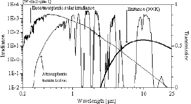
The most dominant source in passive remote sensing of plumes is sunlight. However, other sources will have to be considered, particularly in the LWIR. These other sources include downwelled solar radiance (skylight), reflected radiance from the earth (earthshine) and other background objects, atmospheric thermal self-emission and thermal self-emission from the earth.

Figure 3-1: Plot of Atmospheric Transmission, Solar Irradiance and Thermal Self-Emission.

In the visible and near-IR (NIR) regions, sunlight is the dominant source of photons. In the MWIR, both sunlight and self-emission are of the same order of magnitude, while in the LWIR the impact of solar irradiance is negligible.

Solar and Self-emissive Radiation Incident on the Plume

(2,3)

The solar spectral irradiance onto the plume can be expressed as

[W/m2],(3-1)

where E′_Sλ is the exo-atmospheric irradiance, τ′ is the optical depth of the intervening atmosphere and σ is the solar declination (zenith) angle. This will be the only source of direct incident radiation.

The atmosphere also scatters sunlight onto the plume. This is referred to as downwelled solar scattered radiance (LDS), or skylight. It is a function of both the azimuthal (φ) and zenith (σ ) directions. MODTRAN, an atmoshperic

radiation code, is used to calculate the downwelled radiance at preset angular increments for φ (from 0º to 360º) and for σ (from 0º to 90º) integration over the hemisphere will give the total downwelled radiance onto the plume.(4) This will be considered a diffuse source of radiation. There is also upwelled solar scattered radiance, LUS. This will not interact with the plume, but it will contribute to the final radiance at the sensor (usually as noise).

Direct sunlight is also diffusely reflected from the ground (earthshine):

[W m-2sr-1] (3-2)

where r_E

is the diffuse Lambertian reflectance of the ground. This will be another source of diffuse radiance onto the plume. While there are other solar sources such as reflected skylight from the ground, these will be ignored due to their insignificant contributions. These terms may be added in the future if there is the desire to account for all possible sources.

Thermal self-emission becomes a significant source of radiation in the MWIR and LWIR. All self-emissive sources are considered diffuse incident radiation. One such source is downwelled thermal self-emission from the atmosphere (L_Dε).

angular increments and upon integrating over the hemisphere the total atmospheric emission onto the plume is found.(4)

Upwelled emission from below the plume will be considered negligible. Upwelled self-emission from the intervening atmosphere between the plume and sensor (LUε) will contribute to radiance reaching the sensor.

There is also thermal emission from the earth and background LEε. The radiance is modeled using Planck’s formula:

[W m-2µm-1](3-3)

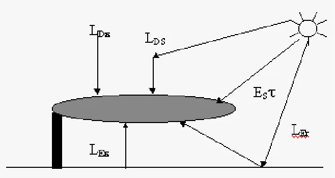
where h, c, k and T are Planck’s constant, the speed of light, Boltzmann’s constant and the temperature in Kelvin, respectively. It is then multiplied by the emissivity of the object, usually defined as one minus the reflectivity. Other minor sources such as atmospheric self-emission reflected from the earth onto the plume are considered negligible. Figure 3-2 shows the main sources of radiation onto the plume.

Figure 3-2: Main Radiation onto a Plume.

Radiation from the Plume

There are two main sources of radiation from the plume reaching a sensor. The first is scattered radiance, which may be either single or multiple scattering. Only direct solar irradiance is considered for single scattering. One reason for this is that scattering is only significant in the visible and NIR spectra where the predominant source are direct solar irradiance. The other reason is that if enough scattering occurs for these other sources to make a significant

contribution, then multiple scattering needs to be considered.

Each region of the plume has an associated angular scattering coefficient β(λ,θ). The element of scattered radiance to the sensor along the traversing sensor ray in that region is:

[W m-2sr-1] ,(3-4)

where θ is the scattering angle, τp1

[W m-2sr-1],(3-5)

where is the transmission from the entrance of the solar ray to the mid-point of the sensor ray in that region and

is the transmission from the mid-point to the point where the ray enters that region (see Figure 3-3).

Figure 3-3: Scattering within the Plume.

The assumption that the scattering angle remains constant over l can be made since the extent of the plume is small

compared to the angular distance to the sensor and sun. The assumption that , and remains constant over l can be made since for single scattering the optical depth must be small (< 0.3). Almost all cases of single scattering will occur only in single region plumes.

For multiple scattering, the two-stream approximation for radiative transfer will be used. Though there are several limitations to this approach, it is a suitable first cut at modeling multiple scattering in plumes. The scattered radiance from direct solar irradiance is

[W m-2sr-1],(3-6)

where r_dir

is the diffuse reflectivity for direct incident radiation as calculated from the two-stream approximation. For diffuse incident radiation, such as the integrated downwelled solar scattered or self-emission, the scattered radiance is

[W m-2sr-1],(3-7)

where r_dif

is the diffuse reflectivity for diffuse incident radiation. Note that both reflectivities are dependent on the sun-plume-sensor geometry, in addition to the plume characteristics. With a multiple scattering plume, the

transmission from the two-stream approximation is used. This accounts for forward-scattered radiation that emerges in the same direction as the original radiation and thus is added back in. There are three types of transmission values: the first is analogous to the Beer-Lambert law except for the forward scattering being considered. This is for direct transmission (τ_DB) of the direct incident solar radiation. The second is diffuse transmission (τ_dir) for direct incident radiation. This represents multiply scattered light emerging from the plume diffusely (i.e., not in the original

direction of the incident radiation). The third is diffuse transmission (τ_dif) for diffuse incident radiation. This is similar to τ_dir

The plume will also radiate from thermal self-emission. The temperature of the plume determines the amount of blackbody radiation (LPBB) from Planck’s equation. The emissivity is determined from Kirchoff’s equation:

(3-8)

The product of the blackbody radiation and emissivity gives the amount of thermal self-emission.

3.3 Downward Looking Sensor

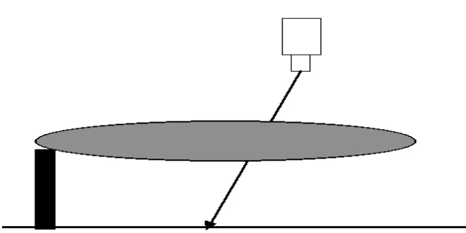
Figure 3-4: Downward-looking Sensor Geometry.

An airborne or satellite sensor looking down will have radiance sources from the intervening atmosphere. Figure 3-4 shows the geometry for a downward-looking sensor.

In the visible region the radiance reaching the sensor is:

[W m-2sr-1],(3-9)

where the first term is the reflected sunlight off the background pixel, the second is the scattered sunlight from the plume, the third is the scattered skylight from the plume and the final term is the upwelled solar scattered radiance. The atmosphere under the plume is considered negligible. Also any reflection of the plume off the background is also considered negligible. In the LWIR, the radiance is:

[W m-2sr-1]. (3-10)

The first term is the earth's thermal self-emission, the second is the plume's self-emission, the third is the scattered downwelled atmospheric self-emission and the last term is the upwelled radiance from the atmosphere. In the MWIR the radiance is:

[W m-2sr-1].(3-11)

from the background, are considered negligible.

Experimental Design and Methods

The purpose of this research is to study the spectral sensitivity characteristics of an air-based sensor. Incorporating the JPL plume simulation in the synthetic image generated scene, observations of the spectral signature of a gas plume and its interaction with various spectrally specific backgrounds were made.(5) Trichloroethylene (C₂HCl₃) is the gas used in this study.

Figure 4-1: Spectral Signature of Trichloroethylene (C2HCl3).

Looking at the signature of C2HCl3

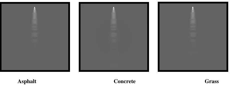
we can see that there are three dominant peaks, all of which occur in the long wave infrared (LWIR) region of the electromagnetic spectrum. Regions in the 8 -12µm regions are well suited for remote sensing because of the relative transparency of the atmosphere at these wavelengths [See Figure 3-1]. Because the three dominant peaks occur within the 10-13.5µm region of the spectrum we will concentrate on these wavelength regions in this research. Three homogeneous backgrounds were used; asphalt, concrete and grass. Once the simple cases are examined, the

interaction of the plume with a real world

scene will be examined. The spectral radiance of the plume will be collected at specific distances as it travels

downwind from the stack exit. Once all the data is collected, a series of inversion algorithms designed to qualify and quantify the plume will be performed.

JPL Plume Model

The JPL plume model is designed to model gas plumes released from factory stacks. The user determines the effluents contained in the plume and multiple effluents are possible. While not designed to model cooling tower plumes, water droplets can be specified as a plume constituent

geometry parameters. Table 4-1 shows the parameters in each category.

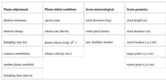
Table 4-1: Input Parameters for JPL Plume Model.

Plume adjustment Plume initial conditions Scene meteorological Scene geometry

dilution minimum species type wind direction (deg) stack height (m)

dilution change release rate (lbs/hr) wind speed (knots) stack diameter (m)

Sampling step size plume release temp. (F° ) atm. Stability number stack location x,y,z (m)

contrast contribution release velocity (m/s) target point x,y,z (m)

number planes modeled sensor point x,y,z (m)

Sampling time interval

The plume adjustment parameters govern the shape and characteristics of the plume. For example, decreasing the dilution change

parameter will increase the dilution factor. Increasing the number of plume planes will increase the length of the plume downwind. The sampling step size is given as a fraction of the stack diameter. These parameters can be adjusted so as to match the plume model with any available experimental data.

The plume initial conditions

parameters determine the initial conditions of the plumes. Multiple species type and their individual release rate can be specified. The molecular weight of each species is also needed. The release rate, release velocity and stack diameter will impact the downwind VMR and column density.

The scene meteorological

parameters determine the meteorological conditions at the stack. This can be described either through time-varying conditions or as a time-averaged condition. If the time-averaged parameters are used, a plume with constant shape results. If time-varying conditions are used, then the user must supply the parameters as they vary over time. This filename is specified in the Plume_Input

file. By using time-varying parameters, the plume can be given some texture and made to puff. The wind speed controls how much the plume is bent over. The atmospheric stability number determines how quickly the plume disperses; the lower the number the lower the dilution downwind.

The scene geometry parameters determine how the plume is to be sampled

Inverse Algorithms

(6)

A term used to determine how visible the plume is against the background is the contrast ratio. This is defined as:

(4-1)

where is L_Plume is the radiance reaching the sensor from a plume pixel and L_Background is the radiance from a background pixel. Notice this is spatial in nature and all values are at the same wavelength. A spectral contrast ratio can be similarly defined where the background radiance is from the same pixel, but at a different wavelength.

One possible way to determine the signature of the plume is to do a simple background subtraction. While this will show the spectral regions where species within the plume are absorbing, the band shape will be distorted. This is because the plume both absorbs and emits radiation. In addition background subtraction leaves the signal in sensor digital counts and does not provide a direct way to calculate the plume density. Aerospace Corp. (6) has developed a way to overcome these shortcomings through a special ratio technique developed for up-looking sensors. The plume transmission is determined by inverting the radiance equation 4-2.

[W m-2sr-1](4-2)

Since scattering is negligible in gases and the spectral bands of interest are in the IR, the radiance reaching a ground-based sensor is

(4-3)

The assumptions are that the atmosphere below the plume is negligible and that Kirchoff’s Law is used to relate the plume emissivity and transmission. The downwelled radiance is determined by measuring a background pixel that does not contain the plume. LPBB

is obtained from an ambient black plate spectrum (the plume and the black plate are assumed to be at the same temperature). The transmission of the plume can be expressed as this special ratio:

(4-4)

For an optically thick plume, the radiance reaching the sensor will be close to the blackbody radiance at the plume temperature.

For an airborne sensor the same method is applied, with a few added terms. Again neglecting scattering in the IR and solar effects, the radiance reaching the sensor is

(4-5)

(4-6)

L_Uεand τ_atm can be derived either through MODTRAN or in-scene techniques and L_Eεis obtained from a background (earth) pixel. (4)

Once τ_P is calculated then the species concentration can be determined. τ_P is first converted into absorbance through eqn. 4-6:

(4-7)

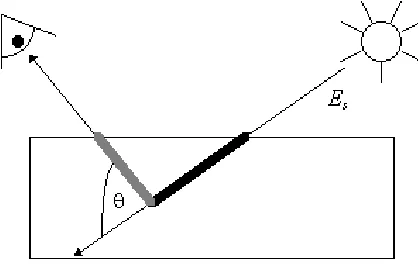
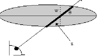
After the absorbance is known for that particular pixel, the plume depth needs to be estimated. This is where the spatial information of a hyperspectral sensor is useful. A first-cut assumption is that the plume is rotationally symmetric around the plume axis. Thus the width of the plume is same as the depth, assuming the sensor LOS through the plume is perpendicular to the plume axis. If the LOS is at an angle, then the plume depth can be

estimated as where w is the plume width perpendicular to the plume axis and θ is the LOS of the sensor to the plume. Figure 4-3 illustrates the geometry.

Figure 4-3: Method of Estimating Plume Depth.

Once the plume depth is estimated, then the VMR is found by:

[ppm].(4-8)

A_database is the spectral absorbance for the particular gas taken from the database. Column_density_database is the

column density at which the gas was measured. The 0.434-1 is a constant derived from 1/ln(10). This process can be done for each plume pixel in the image. This way the VMR can be estimated spatially over the entire plume based on the radiance values.

Results and Analysis

Figure 5-1: Emissivity Curve of Asphalt, Concrete and Grass.

A set of meteorological conditions was also used to simulate wind velocity, direction and atmospheric conditions over 2 second intervals.

Asphalt Concrete Grass

Figure 5-2: Simple Cases of Differing Background (11.8µm).

Figure 5-3. Spectral Signature of Plume Downwind (Asphalt).

Figure 5-5: Spectral Signature of Plume Downwind (Grass).

The absorbance features of the spectra seem to decrease exponentially at further distances downwind. It appears that after 45m peaks that assist us in identifying the chemical are gone. This is not the case. The absorbance curve sits on top of the blackbody curve of the background; which in this case is grass (300K). By taking the background out we will be left with the chemical spectra. Using simple background subtraction we more clearly see the signature downwind. By taking a non-plume pixel and subtracting it out from the plume pixel a more familiar spectral signature of the gas can be seen. The results of this are plotted below.

Figure 5-7: Spectral Signature of C2HCl3 (Concrete).

Figure 5-8: Spectral Signature of C₂HCl₃ (Grass).

Figure 5-9: Spectral Signature of Plume Further Downwind (Asphalt).

Figure 5-11: Spectral Signature of Plume Further Downwind (Grass).

At 45 meters the spectral signature of the plume seems to exhibit similar characteristics of the other spectra at this distance. In all three cases the signature of the plume drops dramatically as it travels from 45 meters to 75 meters downwind. Asphalt and concrete seem to attenuate the spectral signature of the plume similarly. As for grass, the spectral features decrease as we travel further downwind but at 100 meters, where we expect the absorption features to be at its weakest, the spectra seems to shifted upward. This is best illustrated in Figures 5-12 and 5-13.

Figure 5-13: Absorbance Features Comparison at 100 meters.

The contrast ratio (eqn. 4-1) was calculated for the 11.8µm absorption feature as a function of distance downwind. The contrast ratio of all the backgrounds was plotted on Figure 5-14. This graph allows use to view how spectrally visible the plume becomes as it continues downwind.

Figure 5-14: Spectral Contrast Ratioof Plume to Background.

Figure 5-15: Meteorological Effect on Plume Simulation.

Using the meteorological conditions in the plume a more realistic plume can be simulated. The puffing which occurs is attributed to the change in wind direction. As it travels downwind, the plume dissipates but exhibits a puffing characteristic as it travels further from the stack. This results in regions of the plume where there may be high

column density followed by a low column density. At 100 meters, because the column density is low, the signature is attenuated more by the background. This is due to the plume's entrainment of the ambient air.The signature of the plume is diminished as more of the air is entrained and more of the background is exposed.

Figure 5-16: Simulation of Complex Scene (Nevada Test Site).

For a complex scene a simulation of the Nevada Test Site was used. Fifty different material were incorporated to assemble the scene. Because of this we can not simply subtract the background to attain the absorption spectra of the chemical effluent. The plume/background interaction is far more complex than that of the simple homogeneous case. Each material modifies the spectral signature of the plume but with different weighting. A material closer to the plume attenuates the spectra more so than a material situated 25 meters away. This may prove to be a problem when it comes time to identify the chemical constituents of the plume; especially at a much lower resolution. In the case where the resolution is far less, other techniques such as spectral un-mixing may be used to isolate the features of the chemical from the background. Due to time restrictions we will not utilize the pre-mentioned technique in attempts of identifying the spectral signature of the plume at a lowered resolution. Since the gas is known we can forego the task of identify the effluent but instead explore the plume's interaction with the real background. Figure 5-17

Figure 5-17: Spectral Signature in Complex Scene (C₂HCl₃).

Figure 5-18: Spectral Signature as a Function of Distance.

Figure 5-19: Absorption Peak of C₂HCl₃(11.8µm).

Conclusion

The purpose of this research was to apply the plume model against a variety of different backgrounds. By varying the backgrounds and increasing the complexity of the scene we can investigate its interaction with the plume. As part of the increase in complexity, a more realistic scene containing appropriate scene elements was produced. Along with this series of image backgrounds, various plume constituents, concentration and atmospheric conditions will also be generated. These images need then be used to test the ability of inversion algorithms to study plume chemical constituents.

Inversion algorithms designed to determine effluent concentration is used to test these images to determine their accuracy and robustness. Sensitivity studies using passive remote sensing can provide information on plumes over a wide spectral band and with the use of multispectral image fusion additional information can be yielded. These studies are done on the plume-background contrast based on changes in the plume characteristic.

The plume's interaction with simple and complex background was investigated. Simple background interaction returned nice well behaved effluent spectra. The attenuation of the plume by the background was not apparent until the plume was further downwind. By incorporating the meteorological file to the plume simulation it increases the complexity of the interaction between the plume and the background. The absorption peaks were compressed with the incorporation of a complex background. The peaks were not as apparent compared to the effluent spectra of the simple cases. Once downwind, the plume temperature reaches ambient and the background and plume interaction is more noticeable.

These simple scenarios may prove to be useful in the future but there are still many issues to be addressed before relying on these experiments. In order to understand the interaction of the background with the plume it is wise to begin with the most simplistic cases. One drawback of the simulations done in this experiment may be the cases were too simplistic. Usually there are a large number of emissivity curves associated with every object. This is because there are variation in the emissivity curves depending on how or when the data was collected. Though DIRSIG has the capability to incorporate a large library of emissivity curves for each material, the simulation done in this experiment only used a single curve for each material.

can only guess at the accuracy of the simulation. To validate the finding it is essential that there is some data that we can refer to as accurate and use for comparison purposes to gage our results.

One of the questions this experiment could have answered or even suggested is the critical distance. The critical distance is the point at which the plume is undetectable. As the plume exits the stack it immediately begins to entrain air. As the plume moves further downwind, it entrains more of the ambient air and thus diminishes the spectral signature of the chemical released by the plume. By examining the spectral contrast ratio of the plume as a function of downwind distance we were able to get an idea of where the critical point may be for this set of specified

condition. From this experiment, it suggests that the critical distance lies between 60 and 70 meters downwind from the stack. These results are questionable due to the problems associated with the physics of the plume as it exits the stack.

Though the results of the experiment reveal some information about the interaction of the plume and the background, they are too clean

in nature. They are only simulations therefore we cannot expect them to mirror conditions of the real world. Because we cannot does not mean that we can't try. DIRSIG enables the user to control many variables and conditions in attempts to mimic the real world. Conditions too simple can only lead us to question our results. This was where the experiment was flawed. The conditions were too simplistic. Lacking truth data to compare our results with only contributes to the conundrum.

Since this experiment many changes has been done to improve and fix some of the bugs associated with the plume model. This will be useful in the future if anyone would like to investigate the tradeoffs between scene resolution and plume detectability. This experiment would be useful in cases where there are many objects/materials within the scene.

Evaluation of Inversion Algorithms on DIRSIG Generated Plume Model

Simulations

Chia Y. Chang

1. Schott, J. et. al., DIRSIG: Description, Enhancements, and Validation, RIT/DIRS Report 92/93-51-146, 1993.

2. Kuo, S. Didi, Synthetic Image Generation of Factory Stack and Water Cooling Tower Plumes, Ph.D. Dissertation , Rochester Institute of Technology 1997

3. Schott, J., Remote Sensing: The Image Chain Approach, Oxford University Press, 1996.

4. Anderson, G. P., et. al., FASCODE/MODTRAN/LOWTRAN: Past/Present/Future, 18th Annual Review Conference on Atmopsheric Transmission Models, 1995.

5. D. A. Haugan, Lectures on Air Pollution and Environmental Impact, American Meteorological Society (AMS), Boston, 1975.

6. Polak, M. L., Hall, J. L., and Herr, K.C., Passive Fourier-Transform Infrared Spectroscopy of Chemical Plumes: An Algorithm for Quantitative Interpretation and Real-Time Background Removal, Applied Optics, 5406-5412, 34, 1995.