Progress in numerical modeling of non-premixed combustion
Thesis by
Yuan Xuan
In Partial Fulfillment of the Requirements for the Degree of
Doctor of Philosophy
California Institute of Technology Pasadena, California
2014
c
2014
Acknowledgements
Funding from the U.S. Department of Energy-Basic Energy Sciences (DE-SC006591) is gratefully acknowledged. This research used computing resources of the National Energy Research Scientific Computing Center, which is supported by the Office of Science of the U.S. Department of Energy under Contract No. DE-AC02-05CH11231. This research also used the computing resources of the Extreme Science and Engineering Discovery Environment (XSEDE), which is supported by National Science Foundation grant number OCI-1053575.
This work has benefited greatly from discussions with many graduate students, post-doctoral fellows, and professors at the Graduate Aerospace Laboratories, among them, Siddhartha Verma, Phares Carroll, Gerry Della Rocca, Jason Rabinovitch, Shyam Menon, Pauline Vervisch, Remy Mevel, and Professor Beverley McKeon. I also deeply acknowledge Dr. Christopher Shaddix at San-dia National Laboratories and Professor Michael Mueller at Princeton University, Professor Chris-tian Hasse at Freiberg University of Mining and Technology, and Professor Nobert Peters at RWTH Aachen for their valuable comments and fruitful discussions.
Abstract
Progress is made on the numerical modeling of both laminar and turbulent non-premixed flames. Instead of solving the transport equations for the numerous species involved in the combustion process, the present study proposes reduced-order combustion models based on local flame structures. For laminar non-premixed flames, curvature and multi-dimensional diffusion effects are found critical for the accurate prediction of sooting tendencies. A new numerical model based on modified flamelet equations is proposed. Sooting tendencies are calculated numerically using the proposed model for a wide range of species. These first numerically-computed sooting tendencies are in good agreement with experimental data. To further quantify curvature and multi-dimensional effects, a general flamelet formulation is derived mathematically. A budget analysis of the general flamelet equations is performed on an axisymmetric laminar diffusion flame. A new chemistry tabulation method based on the general flamelet formulation is proposed. This new tabulation method is applied to the same flame and demonstrates significant improvement compared to previous techniques.
Contents
Acknowledgements iii
Abstract iv
Contents v
List of Figures xi
List of Tables xvii
1 Introduction 1
1.1 Background . . . 1
1.2 Computational modeling of non-premixed reacting flows . . . 2
1.3 Direct numerical simulations . . . 3
1.4 Chemistry tabulation. . . 6
1.5 Steady-state laminar diffusion flamelets . . . 7
1.6 Flamelet-based modeling of laminar non-premixed flames . . . 9
1.7 Flamelet-based modeling of turbulent non-premixed flames . . . 11
1.8 Objective and outline . . . 13
2 Governing equations and numerical solver 15 2.1 Governing equations . . . 15
3 Multi-dimensional effects in the prediction of sooting tendencies 19
3.1 Direct numerical simulations with finite-rate chemistry . . . 20
3.1.1 Burner configuration and running conditions . . . 21
3.1.2 Chemistry model . . . 22
3.1.3 Numerical set-up . . . 22
3.1.4 Results . . . 24
3.2 Conventional laminar diffusion flamelet results . . . 26
3.2.1 Laminar diffusion flamelet equations . . . 26
3.2.2 Results . . . 27
3.3 Derivation of modified flamelet equations . . . 29
3.3.1 Preliminary considerations . . . 30
3.3.2 New mapping . . . 30
3.3.3 Effects of the different terms . . . 32
3.3.4 Closure of the modified flamelet equations . . . 32
3.3.5 Determination of the aggregate scalar dissipation rate . . . 34
3.3.6 Simulation procedure . . . 35
3.3.7 Validation . . . 36
3.4 Sooting tendency analysis . . . 37
3.4.1 Doped flame versus undoped flame . . . 37
3.4.2 Sooting yield versus PAH dimer production rate . . . 38
3.4.3 Numerical YSI . . . 40
3.4.4 Discussion. . . 41
4 Modeling curvature effects in diffusion flames using a laminar flamelet model 43 4.1 Derivation of the flamelet equations with curvature . . . 44
4.1.1 Conventional laminar diffusiton flamelet model . . . 44
4.1.2 Generalized flamelet coordinate transformation . . . 45
4.1.4 Previous flamelet formulations with curvature effects . . . 48
4.1.5 Convection in mixture fraction coordinate system. . . 48
4.1.6 One-dimensional curved flamelets. . . 50
4.1.7 Magnitude of curvature term . . . 51
4.2 Curved flamelet modeling . . . 54
4.2.1 Tubular counterflow diffusion flames . . . 54
4.2.2 Unsteady spherical inter-diffusion layer. . . 57
4.2.3 Summary . . . 58
4.2.4 Flamelet solutions with curvature effects. . . 59
4.3 Curvature effects in multi-dimensional configurations . . . 61
4.3.1 Tangential diffusion . . . 62
4.3.2 Curvature-induced convection . . . 63
4.3.3 Budget analysis. . . 65
4.3.4 Comparison between full chemistry results and tabulated chemistry predictions 68 4.4 Discussion . . . 70
5 A flamelet-based chemistry tabulation method for polycyclic aromatic hydrocar-bons in turbulent non-premixed flames 76 5.1 Turbulent effective Lewis numbers . . . 77
5.2 Unsteady Lagrangian flamelet modeling . . . 80
5.2.1 Unsteady flamelet equations. . . 80
5.2.2 Scalar dissipation rate . . . 81
5.2.3 Chemistry tabulation methods . . . 82
5.2.3.1 Method I: Chemistry tabulation based on steady-state flamelets . . 82
5.2.3.2 Method II: Chemical source term tabulation . . . 82
5.2.3.3 Method III: Flamelet-based relaxation model for PAH molecules . . 83
5.3 Turbulent effects modeling. . . 84
5.3.2 Perturbation and relaxation procedure . . . 85
5.3.3 Flamelet configuration and parameters. . . 85
5.4 Relaxation behaviors . . . 87
5.4.1 Overview of steady-state flamelets . . . 87
5.4.2 Initial evolution. . . 89
5.4.3 Relaxation time scales . . . 91
5.4.4 Relaxation of radicals and small species . . . 91
5.4.5 Relaxation of aromatic species . . . 92
5.5 PAH relaxation model . . . 95
5.5.1 Previous one-step relaxation model . . . 96
5.5.2 Proposed multi-step model . . . 96
5.5.3 Discussion. . . 98
5.5.4 Validation . . . 100
6 Effects of aromatic chemistry-turbulence interactions on soot formation in a tur-bulent non-premixed flame 102 6.1 Numerical algorithms . . . 103
6.1.1 Soot model . . . 103
6.1.2 Gas-phase chemistry model . . . 104
6.1.3 Radiation model . . . 105
6.1.4 LES closure . . . 107
6.1.4.1 Transport equations . . . 107
6.1.4.2 subfilter modeling . . . 107
6.1.4.3 Equation of state . . . 109
6.1.4.4 Subfilter variance modeling . . . 111
6.1.5 PAH relaxation model . . . 111
6.2 Choice of the flame under study. . . 113
6.2.2 Experimental studies of sooting turbulent non-premixed flames . . . 114
6.2.3 Selected flame . . . 115
6.3 Simulation details . . . 117
6.3.1 Flame configuration . . . 117
6.3.2 Numerical set-up . . . 118
6.3.2.1 Boundary conditions. . . 118
6.3.2.2 Fully-developed pipe flow simulation . . . 119
6.3.2.3 Choice of the computational domain and grid resolution for flame simulation . . . 122
6.3.2.4 Generation of the flamelet library . . . 128
6.3.2.5 Preliminary verification . . . 128
6.3.3 Computational cost . . . 129
6.4 Results and discussion . . . 130
6.4.1 Instantaneous fields . . . 130
6.4.2 Mean soot profile . . . 131
6.4.3 Effects of PAH chemistry-turbulence interaction . . . 133
6.4.4 Soot volume fraction fluctuations . . . 137
7 Conclusions and future directions 139 7.1 Conclusions . . . 139
7.2 Modified flamelet equations for YSI predictions . . . 139
7.3 Curved flamelet formulation . . . 140
7.4 Chemistry-turbulence interactions . . . 141
7.5 Effects of chemistry-turbulence interactions on soot formation . . . 142
7.6 Recommendations for future work . . . 143
Appendix A Modified flamelet equations on the centerline of axisymmetric laminar
Appendix B Curved flamelet formulation 145
B.1 Detailed derivation of the flamelet equations including curvature effects . . . 145
B.2 Comparisons with the flamelet equations proposed by Williams . . . 148
B.3 The complete curved flamelet equations . . . 150
Appendix C Review of the derivation of flamelet equations including curvature effects 151 C.1 Galilean transformation . . . 151
C.2 Coordinate transformation rules. . . 153
C.3 One-dimensionality . . . 154
C.4 Tangential diffusion . . . 155
C.5 Summary . . . 156
Appendix D Description of the simulation code: NGA 158 D.1 Treatment of the convective and viscous terms . . . 158
D.2 Time-integration . . . 159
Appendix E Description of the FlameMaster code 163 E.1 General Description . . . 163
E.1.1 Thermodynamic Properties . . . 163
E.1.2 Reaction Rates . . . 164
E.1.3 Transport Properties . . . 164
E.1.4 Mixture-averaged properties. . . 165
E.2 Laminar diffusion flamelet calculations . . . 166
List of Figures
1.1 Recent DNS studies of non-premixed reacting flows with finite-rate chemistry. . . 3
1.2 Schematic of the combustion ofn-heptane. The part to the left of the dash line does not include any aromatic chemistry. . . 4
1.3 Different categories of chemical kinetics integration strategies.. . . 7
1.4 Illustration of flamelet database for chemistry tabulation generated using the solutions to steady-state flamelet equations. . . 8
3.1 Schematic of the diffusion flame and burner configuration.. . . 21
3.2 Axisymmetric structured mesh used for the flame simulations. . . 23
3.3 Temperature, methane mass fraction, and acetylene mass fraction fields from the 2D direct simulation. Dashed lines indicate the location of the stoichiometric surface. . . 24
3.4 Centerline gas temperature. . . 25
3.5 Scalar dissipation rate, temperature, and axial velocity profiles extracted from the 2D simulation along the centerline plotted in mixture fraction space. . . 28
3.6 Comparison of species mass fraction in mixture fraction space between the DNS and the conventional flamelet model. . . 29
3.7 Schematic of the diffusion process. The dashed lines represent the mixture fraction iso-contours, and the dash-dot lines representφiso-contours. . . 32
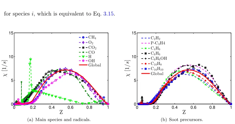
3.8 Aggregate scalar dissipation rates for species of interest and the global fitted one. . . 34
3.10 Dopant (C6H6) mass fraction profiles on the centerline of flames with dopant calculated
using conventional and modified flamelet models. . . 38
3.11 Comparison between the flame with and without dopant (C6H6) for OH radical, C2H2,
and PAH dimer production rate. . . 39
3.12 Linear relation between the measured YSI in the literature and the numerically com-puted YSI. . . 41
4.1 Schematic of the coordinate transformation.. . . 45
4.2 Functional dependence of scalar dissipation rate on mixture fraction. Red solid line: Eq. 4.23. Black dash line: Eq. 4.24. Blue dash-dotted line: Eq. 4.25. . . 52
4.3 Two basic configurations representing local 1D flamelet structures in turbulent reacting flows. . . 55
4.4 Mixture fraction, scalar dissipation rate, and curvature profiles for steady-state coun-terflow tubular flames.. . . 57
4.5 Mixture fraction, scalar dissipation rate, and curvature profiles for a spherical laminar unsteady mixing layer.. . . 58
4.6 Comparison of H2, C2H2, and C6H6 mass fractions between curved and flat flamelets.
For comparison, the maximum gradient of mixture fraction is calculated to be 103m−1,
leading to a lower limit of the estimated ratio of φ = 1.94 (Eq. 4.27) for the curved flamelets withκ=±200[m−1]. . . . . 60
4.7 Sensitivity of C6H6 concentration to curvature effects and scalar dissipation rates at
mixture fractionZ = 0.3. . . 61
4.8 Comparison between the flamelet solutions for the mass fraction of H2obtained using
constant and mixture-fraction-dependent (Eq. 4.35) curvatures. . . 61
4.10 Ratio of the curvature-induced convective term over the normal convection term (Eq. 4.29) extracted from the numerical results (on the left) and the mixture fraction contour plot (on the right). The white line denotes the location of the flame front. . . 64
4.11 Comparison of different convective velocities in mixture fraction space. The ”original term” being plotted corresponds to the expression in Eq. 4.12, the ”curvature term” being plotted corresponds to the expression in Eq. 4.13, and the ”DNS results” being plotted corresponds to the sum of the two previous terms, as expressed by Eq. 4.10. . 65
4.12 Budget analysis on the flame centerline for three characteristic species. . . 72
4.13 Budget analysis on a flame radius for three characteristic species. The radial cut corresponds to the black line in Fig. 4.10. . . 73
4.14 Comparison between budget analyses based on simulation results obtained using two different grid resolutions. . . 74
4.15 Mass fraction profiles of several representative species on the flame centerline.. . . 75
5.1 Measured conditional means of species mass fractions (symbols) compared with laminar opposed-flow flame (flamelet) calculations including full molecular transport (dashed lines) or equal diffusivities (solid lines). These figures are taken from Barlowet al.[58]. 79
5.2 The burning branch of the S-shaped curve for the flame configuration considered. The solid line corresponds to the maximum C6H6 mass fraction in the solutions of the
steady-state flamelet equations. The solid arrows indicate the abrupt change in scalar dissipation rate to model turbulent effects, and the dashed arrows indicate relaxation of the perturbed flamelets towards the final steady-state. PointsAandA0 correspond to two different initial steady-states; points B and B0 correspond to two states after perturbation, and pointCcorresponds to the final steady-state. . . 86
5.3 Mass fraction and chemical source term profiles in mixture fraction space for three representative species in the steady-state flamelet with χst = 20s−1. The chemical
source terms are plotted inkg·m−3s−1. The vertical dashed line represents the location
5.4 Chemical source term distribution of C10H8in two steady-state flamelets. The chemical
source terms are plotted inkg·m−3s−1. . . . . 88
5.5 Time-evolution of the mass fraction for several representative species for a flamelet perturbed from an initial χst = 10s−1 to a final χst = 20s−1. The chemical source
terms are plotted inkg·m−3s−1. The early evolutions are highlighted in the insets on
a linear scale. . . 90
5.6 Time-evolution of the mass fraction and the chemical source term for several represen-tative aromatic species. The chemical source terms are plotted inkg·m−3s−1. . . 93
5.7 Time-evolution of C8H5 and dependence of its mass fraction on the mass fraction of
C6H6 during the relaxation of a flamelet perturbed from an initial χst = 10s−1 to a
final χst = 20s−1. In (b), the initial steady-state is circled. The final steady-state is
indicated by the dashed horizontal and vertical lines. The arrows indicate the paths that unsteady solutions follow as time increases. . . 94
5.8 Modeled chemical production, consumption rates, and overall reaction rates compared to unsteady calculations with full chemistry for C10H8. The chemical source terms are
plotted inkg·m−3s−1. . . . . 97
5.9 Dependence of the chemical source term of C6H6on its mass fraction during the
relax-ation from steady-state flamelets (with various initialχst) to the final steady-state (with
χ0
st= 20) atZC6H6,max= 0.19. The chemical source terms are plotted inkg·m−3s−1.
The initial steady-states are circled. The final steady-state is indicated by the dashed horizontal and vertical lines. The arrows indicate the paths that unsteady solutions follow as time increases. . . 99
5.10 Diagram of reactions leading to the formation of PAH species. . . 99
5.11 Comparison of the time evolution of benzene mass fractions resulting from the detailed chemistry mechanism and the relaxation models. . . 101
6.1 Fast-shutter photographs of ethylene jet flames stabilized on the piloted jet burner.
These figures are taken from Shaddix et al. [94,157,197] . . . 116
6.2 Schematic of the burner configuration. . . 117
6.3 A plane cut of the computational domain at a fixed azimuthal angle (θ= 0). . . 120
6.4 Velocity profile near the pipe wall. . . 121
6.5 LES grid stretching diagram for the three different resolutions. The axial direction is shown in the left column. The radial direction is shown in the right column. The insets in the graphs show zooms of the grid around the fuel nozzle. . . 124
6.6 Time-averaged important characteristics at two locations close to the burner lip. Left column: 2.5 mm downstream of the burner lip. Right column: 5 mm downstream of the burner lip. . . 125
6.7 Time-averaged soot volume faction at two different locations for three different meshes. 126 6.8 A plane cut of the computational domain at a fixed azimuthal angel (θ= 0). . . 127
6.9 Radial profile of the temperature 5 mm downstream of the burner lip. . . 128
6.10 Instantaneous fields of temperature, benzene mass fraction, naphthalene mass fraction, and soot volume fraction. The iso-contour of stoichiometric mixture fraction (indicating the flame front) is shown in solid line. . . 131
6.11 Mean soot volume fraction on the flame centerline. . . 132
6.12 Mass fractions of C6H6and C10H8sampled atZC6H6andZC10H8, respectively, from the relaxation LES are shown in red dots. Mean profiles conditioned on mixture fraction, Z, scalar dissipation rate, χ, and enthalpy defect parameter, H, are plotted in black dash line. The steady-state flamelet solutions are shown in blue solid line.. . . 133
6.14 Time-averaged fields of soot volume fraction. Results obtained using the relaxation model for transported aromatic species are shown on the left half. Results obtained using tabulated aromatic species concentrations are shown on the right half. The iso-contour of stoichiometric time-averaged mixture fraction (indicating the flame front) is plotted in white solid line. Radial profiles are plotted atx/d= 40 andx/d= 140. . . 136
6.15 Mean profiles on the flame centerline. . . 136
6.16 PDFs of soot volume fraction at two locations on the flame centerline. . . 137
List of Tables
3.1 Characteristic parameters for the doped co-flow diffusion flame of McEnally and Pfefferle. 21
3.2 Experimental and numerical sooting tendencies of different species. ∗ Computational
YSI scaled to have the same values as the experimental YSI. . . 41
4.1 Different sets of boundary conditions used in tubular flow calculations. . . 56
5.1 Characteristic time scales and locations of maximum source term (in mixture fraction space) for several representative species for the steady-state flamelet solution with χst= 20s−1. Units are microseconds. . . 92
6.1 Flow parameters for the four piloted ethylene jet flames studied by Shaddix and Zhang.116 6.2 Characteristic parameters for the piloted turbulent jet flame. . . 118
6.3 Details of the inlet conditions for the transported scalar quantities.. . . 119
6.4 Details of the computation meshes tested at different grid resolutions. . . 123
Chapter 1
Introduction
1.1
Background
Energy sustainability and the emission of pollutants will have defining importance in the present century[1]. Historically, the combustion of hydrocarbon fuels has been the principal source of energy due to their high energy density, ease of transport, and relative abundance. Although renewable energy and nuclear power are the world’s fastest-growing energy resources, fossil fuels are estimated to continue to supply almost 80 percent of the world’s energy through 2040, as reported in the International Energy Outlook (2013 report) [1]. Unfortunately, the combustion of fossil fuels not only generates greenhouse gases, but also produces pollutants, such as nitrogen oxides, sulfur dioxide, volatile organic compounds, and nano-sized particles, which can cause severe air quality degradation. Ever more stringent international regulations (e.g. ICAO CAEP2 standards) placed on industrial combustion system emissions make the design of cleaner and more efficient combustion devices a necessity.
The development of clean and efficient combustion systems introduces new challenges, not only in the manufacturing of these systems, but also at a more fundamental level. Although designs of the various combustion systems and their operating conditions may be very different, the turbulent reacting flows involved are subject to the same complexities. First, hundreds of species and thousands of reactions are generally required to describe correctly the chemical aspect of combustion [2,3,4,
the complexity of the systems [6]. Finally, but most importantly, the major complexity found in these combustion systems is due to the intrinsic interactions between small scale chemical processes and large scale flow features. These multi-physics and multi-scale problems are among the biggest challenges in fluid mechanics and are the real limiting factors in the development of more efficient and cleaner energy sources.
1.2
Computational modeling of non-premixed reacting flows
Towards this end, Computational Fluid Dynamics (CFD) has emerged as an indispensable indus-trial analysis and design tool over the past few decades. Its application to the modeling of complex reacting flows has been largely successful [7, 8, 9,10]. However, the predictive capabilities of CFD tools remain limited by the assumptions and approximations made in the modeling of key physical processes. For instance, some modeling procedures that have been widely used in numerical com-bustion were developed for non-reacting, constant density flows [11, 12, 13,14, 15]. These models were developed based on physical arguments with simplifying assumptions, and as a result, have demonstrated inconsistencies when applied in practical situations. This is reflected by the large variety of different combustion models that have been formulated [16] and the continuous effort that has been made to improve these models [6,16].
1.3
Direct numerical simulations
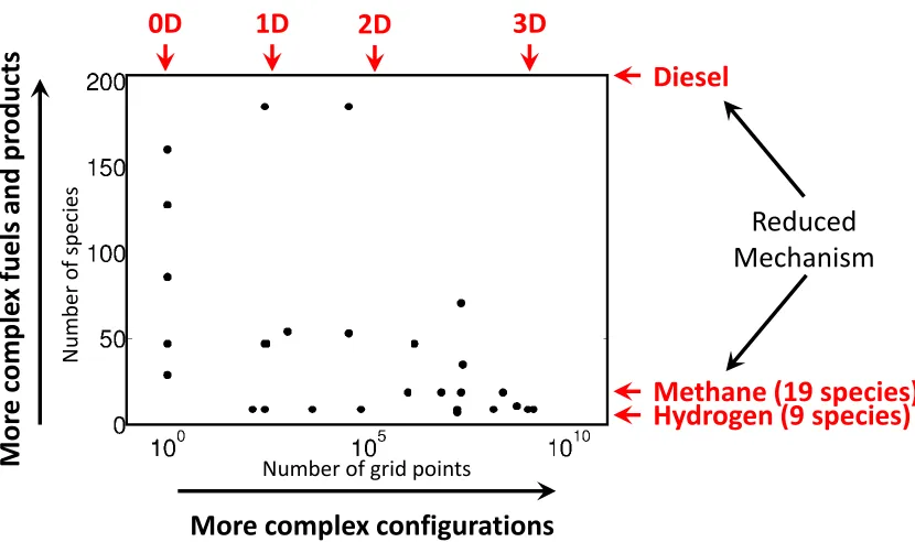
In view of the difficulties in the reduced-order modeling of combustion, Direct Numerical Simulations (DNS) with finite-rate chemistry may seem to be more advantageous, since all the governing equa-tions are solved in these simulaequa-tions, without using any explicit simplifying assumpequa-tions. Indeed, DNS has been employed as a valuable research tool, and recent development in high-performance computing has enabled the application of DNS to more and more complex configurations [18, 19]. Some of the most recent DNS studies of non-premixed reacting flows with finite-rate chemistry are included in the following figure.
Number of grid points
N
u
m
b
er
of
spe
cies
0D
1D
2D
3D
Hydrogen (9 species)
Methane (19 species)
Diesel
More complex configurations
Reduced
Mechanism
Mor
e
c
omp
le
x
fue
ls
and
p
rod
u
[image:20.612.120.535.270.516.2]cts
Figure 1.1: Recent DNS studies of non-premixed reacting flows with finite-rate chemistry.
DNS with finite-rate chemistry has been applied to zero-dimensional homogeneous reactor sim-ulations [20,21] and one-dimensional flame calculations [22, 23,24,25, 26] using detailed chemical mechanisms involving a large number of species. However, only skeleton-level chemical mechanisms have been used in three-dimensional turbulent non-premixed reacting flow simulations [27, 28, 29,
to provide a satisfactory description of complex chemical processes, such as low-temperature com-bustion and soot formation. Overall, the application of DNS with finite-rate chemistry to practical combustion systems using practical fuels (e.g. diesel) as a design tool is still prohibited by the associated extremely high computational cost. This is essentially due to the large number of species and reactions involved in the combustion process and the wide range of time and length scales that need to be resolved in the reacting flow field.
n-heptane
oxygen
carbon monoxide water
carbon dioxide
acetylene ethylene
benzene naphthalene cyclopenta[cd]pyrene
soot
[image:21.612.109.536.212.557.2]Polycyclic Aromatic Hydrocarbons (PAH)
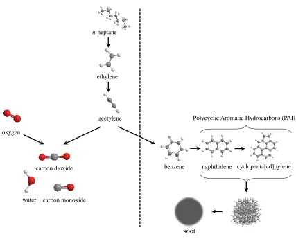
Figure 1.2: Schematic of the combustion ofn-heptane. The part to the left of the dash line does not include any aromatic chemistry.
as ethylene and acetylene. These species react with oxygen to form major combustion products such as carbon monoxide, carbon dioxide, and water. Simultaneously, these intermediate species (e.g.
ethylene and acetylene) react with each other, which leads to the formation of the first aromatic species, namely benzene. Larger aromatic species with more than one aromatic rings, such as naph-thalene, phenanthrene, and pyrene are then formed from benzene [2, 3]. Further collisions between these large aromatic compounds lead to the formation of soot particles [2,3]. Typically hundreds of species and thousands of reactions are required to capture accurately enough the combustion process just described [3,33]. Including such detailed chemical kinetics model burdens substantially reacting flow simulations, due to the large number of transported reactive scalars (i.e. species mass fraction).
Moreover, simulations of reacting flow systems using finite-rate chemistry are extremely challeng-ing due to the multiple time scales involved in the various physical and chemical processes [34,35,36]. In particular, chemistry produces generally very small time scales which make the systems stiff. The high non-linearity in the Arrhenius form of the chemical reaction rate constants in the calculations of the species chemical source terms increases the stiffness of the systems [37]. In addition, for tur-bulent reacting flows, the difference between the thickness of the thin reaction layers (often smaller than the Kolmogorov length scale) and the largest length scale is typically more than three orders of magnitude [32, 31]. As a result, billions of grid points are generally required for the DNS of these flows [30, 38]. Although advanced numerical schemes have been designed for more accurate scalar transport [39,40,41] and more efficient time-integration of stiff chemical source terms [37,20], DNS of reacting flows with complex chemistry under complex configurations are still limited by the current computing resources.
and hydrogen), and have taken into account only the major chemical pathways without considering aromatic species and soot formation (the part to the left of the dash line in Fig.1.2). Typically, the chemical mechanism used for hydrogen combustion in these simulations contains 9 species [30,27,28] and the one used for methane combustion contains 19 species [32, 31, 30, 28]. These mechanisms have been obtained by reducing the number of intermediate species contained in detailed mecha-nisms using chemistry reduction techniques, such as Quasi-State-State (QSS) assumptions [43] and Partial-Equilibrium (PE) approximations [44]. Simulations using these reduced mechanisms are able to capture the major features of the reacting flows under investigation, for instance temperature and major species distributions [32,30,28]. However, reduced chemical mechanisms become insufficient when the combustion of large hydrocarbon fuels (practical fuels) or the formation of complex com-bustion products (soot) is considered. As mentioned earlier, describing accurately such complex chemical processes requires typically hundreds of species and thousands of reactions [2, 3,4]. The efficient integration of detailed chemical kinetics into detailed simulations of reacting flows presents one of the biggest challenges in numerical combustion. One approach to overcome the difficulties dis-cussed above is to use chemistry tabulation. The different categories of chemical kinetics integration strategies discussed are summarized in the following figure.
1.4
Chemistry tabulation
Fewer transported scalars
Fewer transported species
Reduced mechanism
Chemistry tabulation
Full chemical
kinetic mechanism
Reduced-order modeling
Direct integration
[image:24.612.115.527.61.297.2]Direct numerical simulations
with finite-rate chemistry
Figure 1.3: Different categories of chemical kinetics integration strategies.
the system depends on a much smaller number of variables. These variables are often combinations of species concentrations. Multi-dimensional libraries are then used to store the thermochemical states as a function of these variables. These methods are particularly suited for chemical kinetics calculations [46]. Unfortunately, these methods do not include any flow variables (e.g. flow strain rate, flame curvature, and scalar dissipation rate) in constructing the libraries of thermochemical states. As a result, they are limited when applied to non-premixed flames, where the local reacting flow is governed by the balance between chemistry and diffusion [16].
An interesting alternative to chemical-kinetics-based tabulation methods is the flame-structure-based tabulation methods. Such methods include the Flame Prolongation of ILDM (FPI) [47], and the Flamelet-Generated Manifold (FGM) [48]. These methods share remarkable similarities and both rely on the concept of the steady-state Laminar Diffusion Flamelet (LDF) [49,50]
1.5
Steady-state laminar diffusion flamelets
Z, as an independent variable, and using the scalar dissipation rate, χ= 2D|∇Z|2, for the mixing
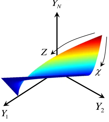
process, was introduced by Peters in 1983 [49] (see Eq.3.1in Section 3.2.1). Historically, Williams was the first to rewrite, under unity Lewis number assumption, the species transport equations by separating the diffusion normal to mixture fraction iso-contours and that in tangential directions [52]. Peters introduced additional simplifications to make use of the flamelet formulation in reacting flow simulations, namely, combustion processes take place in a thin layer close to the flame front, diffusion in the direction parallel to the local iso-surface of mixture fraction is negligible, and the local flame surfaces are essentially flat. Based on these three assumptions, multi-dimensional non-premixed flames can be modeled as an ensemble of piecewise one-dimensional flame structures, termed flamelets. The LDF model has been a popular modeling approach in simulating both laminar non-premixed flames [53,54,55] and turbulent non-premixed flames [56,57,58,59,60,61,22,62]. The distinct advantage offered by the flamelet model, compared to the numerical simulation using finite-rate chemistry model, is that flow properties and chemical kinetics are essentially decoupled [6]. More specifically, steady-state flamelet equations are solved in advance to build a flamelet database. This database is then tabulated as a function of the mixture fraction,Z, and the scalar dissipation rate,χ, as shown in Fig. 1.4. In simulations, the values ofZ andχ are computed locally, based on
N
Y
1
Y
Y
2Z
[image:25.612.237.423.465.674.2]
which the species mass fraction, temperature, and other thermochemical properties are evaluated. As such, the computational cost associated with simulations using flamelet-based tabulated chemistry methods is significantly lower than using finite-rate chemisty, since only the scalar quantitiesZ and
χneed to be calculated locally, without solving the transport equations of all species involved in the chemical mechanism.
1.6
Flamelet-based modeling of laminar non-premixed flames
While being a very powerful modeling framework, the LDF model relies on several key assumptions which may not be valid in all laminar non-premixed flames. Potential impacts of these assumptions require further analysis. Furthermore, these impacts may be present not only in laminar flames, but also in turbulent flames. Yet, they are more pronounced in laminar flames [63].
The first key assumption concerns the species Lewis numbers. In most of the previously referenced studies of turbulent reacting flows [56, 58, 59], unity Lewis number transport has been assumed on the basis that molecular diffusion is negligible compared to turbulent mixing. The influence of non-unity Lewis number transport on turbulence-chemistry interaction has been investigated theoretically, experimentally, and numerically by previous work [63, 64, 65, 66, 67]. The unity-Lewis number assumption is found valid for large-scale mixing in the limit of sufficiently large Reynolds number; and the transition from non-unity (under laminar conditions) to unity Lewis number (under turbulent conditions) was observed for conditional means of species mass fractions in piloted turbulent methane/air jet flames as the Reynolds number was increased [63, 66]. For laminar flames, large deviations have been found in co-flow non-premixed flames when comparing results obtained with unity and non-unity Lewis numbers (e.g. significantly different flame heights and flame widths) [54,68,69].
The second key assumption concerns curvature effects which have been neglected [54, 22, 68,
many species of interest, such as aromatic species, tend to be located farther away from the flame, where the flame can no longer be assumed to be flat, and flame curvature effects could potentially be substantial. The impact of curvature can be further enhanced when mixture fraction iso-surfaces are highly wrinkled by turbulent motions [42]. In other words, curvature effects might be non-negligible when the product of flame curvature by the distance to the flame front is large. Unfortunately, the effects of flame curvature on the flamelet modeling of both laminar and turbulent non-premixed flames still remain not well understood.
The third key assumption concerns the multi-dimensional diffusion effects, i.e. in the direction parallel to the local iso-surface of mixture fraction. These effects have been neglected to achieve the one-dimensionality of the local flame structure. As such, all physical quantities can be parametrized solely by the mixture fraction. However, in a recent study, these multi-dimensional effects were found to be critical in reproducing the complete flame behavior in laminar co-flow diffusion flames [69] and hence might have non-negligible impact on sensitive processes, such as soot formation.
The first one-dimensional laminar flamelet equations were proposed by Peters [49, 50] for flat flames, under unity Lewis number assumption. These equations were extended by Pitsch [70] to take into account non-unity Lewis number effects. Williams proposed a more general flamelet formulation even before Peters without making specific assumptions on the flame structure [52,72]. However, a unity Lewis number was assumed to describe the species transport processes, and the terms corre-sponding to different physical processes were grouped together, making this formulation hardly used in practice. More recently, Kortschik et al.[73] attempted to derive flamelet equations accounting for curvature effects. However, restrictive assumptions were made implicitly in the derivation. As a result, the predicted curvature effects did not show full agreement with the qualitative experimental observations [74]. More precisely, curvature was predicted to still have effects on species with Lewis number close to unity, but those species were observed to be hardly affected in the experiments. Xu
flame curvature using a flamelet formulation for laminar and mildly turbulent non-premixed flames.
1.7
Flamelet-based modeling of turbulent non-premixed flames
Unlike for laminar non-premixed flames, the conventional steady-state LDF model has been found to represent well the local turbulent flame structure, as briefly reviewed at the beginning of Chapter5. Chemistry tabulation based on the steady-state LDF model has been widely applied to Large-Eddy Simulations (LES) of turbulent reacting flows, in which large length scales are resolved and small scale mixing is modeled. LES using LDF-based chemistry tabulation has been applied to a variety of combustion problems of practical interest including the prediction of pollutant emission [7, 8], combustion instabilities [76, 77], and aircraft engine combustion [9, 10]. Although major flame characteristics and main species concentrations are generally well predicted in these simulations, the extension to include more complex chemical products in these simulations should be done with great care.
As aforementioned, one substantial simplification implicitly made by the chemistry tabulation based on steady-state LDF model is that the characteristic chemical time scale is much smaller than that of turbulence. In other words, chemistry is assumed to respond infinitely fast to perturbations from the turbulent flow field. Such assumption may be valid for the major chemical species (reactants and products) as well as radicals (H, OH, O, etc.). For instance, the steady-state LDF model has been shown to represent remarkably well statistically averaged flame properties [63]. However, due to the wide range of time scales involved in turbulent flows and the large time scales characterizing the chemical processes of certain species, transient effects could be substantial. One of such critical processes is the formation of soot particles.
the steady-state LDF model [16, 42]. These observed differences are believed to be a consequence of the rapidly changing turbulent flow field and the slow adjustment of PAH chemistry. Based on the above consideration, turbulence-chemistry interaction needs to be properly treated for PAH molecules.
A series of theoretical studies have been focusing on the chemical response of the flamelets solutions to oscillatory strain rates under various flow conditions [79,80,81,82]. Chemical responses of different species under oscillatory flow rates and strain rates have been also investigated in non-premixed flames numerically [83, 84] and experimentally [85, 86]. The scalar dissipation rate was found to characterize well the unsteadiness of the flow [83]. However, in these studies, emphasis has been placed on major combustion products and a very limited number of intermediate species.
Recent studies have focused on the effects of unsteadiness on the formation of NOxspecies [8,87]
and a relaxation model [8] was proposed for the prediction of their mass fractions in turbulent flames, based on a one-step global reaction. Unfortunately, this relaxation model was only validated
a posteriori. The situation is similar for PAH (i.e.noa priori analysis). Including transient effects for PAH molecules has been attempted by Mueller and Pitsch [22] by using the same model as for NOx [8], despite the fact that PAH species are characterized by an even more complex chemistry
than NOx species. In their work, all PAH molecules were represented by a single lumped PAH
species, and the dependence of the chemical source term on the PAH mass fraction was assumed to be universal for all PAH. While this represents a very good first step, a more reliable model based on a more completea priorianalysis is required to take into account the interactions between chemistry and turbulent unsteadiness. Such model should reflect the multi-step nature of PAH chemistry and distinguish between major PAH species.
1.8
Objective and outline
In view of the issues discussed above, the objective of the current study is to identify the key issues in the flame-structure-based reduced-order modeling of laboratory-scale laminar and turbulent sooting flames, with specific attention placed on the prediction of PAH species. As aforementioned, these PAH species are of critical importance since their concentrations control directly the soot nucleation rates. More precisely, the objectives are three-fold:
1) investigate the effects of flame curvature and multi-dimensional diffusion, and the appropriate-ness of the LDF model in the representation of local flame structures in laminar non-premixed flames,
2) examine the effects of turbulent perturbation on PAH species, and the validity of different chemistry tabulation strategies in the numerical modeling of turbulent non-premixed flames,
3) propose and validate more accurate flamelet-based reduced-order models for the key processes mentioned above and investigate their importance and effects in laboratory-scale flame config-urations.
Chapter 2
Governing equations and numerical
solver
The evolution of the reacting flows under study is governed by the unsteady Navier-Stokes equations and the scalar transport equations. For the simulations undertaken in this work, we adopt the standard zero Mach number assumption that is well justified for many combustion systems and has been used in many previous studies [22,89,90,29,91], as the typical Mach number for both laminar and turbulent diffusion flames is well below 0.1.
2.1
Governing equations
Using the zero Mach number approximation, the continuity and momentum equations are written as
∂ρ
∂t +∇ ·(ρu) = 0, (2.1)
∂ρu
∂t +∇.(ρuu) =−∇p+∇ ·τ, (2.2)
where ρ is the density, p is the pressure, u is the velocity, and τ is the deviatoric stress tensor, defined as
τ=µ
∇u+ (∇u)T
−2
3µ(∇ ·u)I, (2.3)
whereIis the identity matrix andµis the fluid viscosity.
the mixture containingnspecies can be written as
ρcp ∂T
∂t +ρcp∇ ·(Tu) =∇ ·(ρcpα∇T) + X
i
cp,iρDi∇Yi· ∇T+ ˙ωT −q˙rad, (2.4)
where ˙ωT includes heat source terms due to chemical reactions, α is the thermal diffusivity, Di is
the molecular diffusivity of speciesi, and ˙qrad encompasses all heat losses due to radiation.
Flame radiation is modeled using the RADCAL model [92]. This model relies on the assumption of optically thin medium, which is a reasonable assumption for the laboratory-scale laminar and turbulent flames considered [68, 92, 93, 94]. The radiating species considered in these flames are CO2, H2O, CH4, and CO. This model uses the following expression for the rate of heat transfer per
unit volume due to radiation [54,68,92]
˙
qrad=−4σ X
i
piapi(T
4−T
∞4), (2.5)
where σis the Stefan-Boltzmann constant, pi is the partial pressure of speciesi, api is the Planck mean absorption coefficient of speciesi, andT andT∞ are the local flame and background temper-atures, respectively. The Planck mean absorption coefficients are obtained at different temperatures by running RADCAL [95], and fitted to polynomial expressions [92].
For two-feed non-premixed combustion systems (e.g. fuel and oxidizer), the flame structures are generally described by means of a passive scalar Z [16, 96, 97]. This variable is referred to as mixture fraction and ranges from 0 to 1, corresponding to pure oxidizer and pure fuel, respectively. The evolution of this variable is governed by the following transport equation
∂ρZ
∂t +∇ ·(ρZu) =∇ ·(ρD∇Z), (2.6)
whereDis the mass diffusivity forZ. This diffusivity is set to the thermal diffusivity,α. Therefore, the Lewis number forZ
LeZ=
α
is unity.
Assuming non-unity but constant Lewis number and neglecting Soret effects, the transport equa-tion for the mass fracequa-tion of speciesi,Yi, can be written as
ρ∂Yi
∂t +ρu· ∇Yi=∇ ·
ρ α
Lei
∇Yi
+∇ ·(ρYiVc,i) + ˙ωi, (2.8)
where ˙ωi is the chemical source term of speciesi, andLei is the Lewis number of speciesi, defined
as
Lei= α Di
, (2.9)
with Di the mass diffusivity for species i. It was found previously that Soret effects have only
minimal impact on the flame shape and temperature field [98]. The correction velocity Vc,i in Eq.2.8accounts for gradients in the mixture molecular weight as well as ensures zero net diffusion flux. It has the following expression
Vc,i=
α Lei
∇W
W −α
X
j
∇Yj Lej
−α
∇W W X j Yj Lej
, (2.10)
where W = X j Yj Wj −1 (2.11)
represents the mean molecular weight of the mixture.
The above set of equations is complemented by the equation of thermodynamic state
p=ρ 1
WRT,b (2.12)
2.2
Numerical solver
For full scale numerical simulations, the multi-dimensional Navier-Stokes equations and species transport equations are solved using the NGA code [90], using an iterative procedure. The NGA code, using staggered variables, allows for accurate, robust, and flexible simulations of both laminar and turbulent reactive flows in complex geometries and has been applied in a wide range of test problems, including laminar and turbulent flows, constant and variable density flows, as well as Large-Eddy Simulations (LES) and Direct Numerical Simulations (DNS). The numerical method used was developed originally for the simulation of zero Mach number flows with variable density, and have been shown to conserve discretely mass, momentum, and kinetic energy, with arbitrarily high order discretization [90]. This method is an extension of the work of Morinishi et al.[99]. In the simulations presented in this work, second order discretization of the viscous and convective terms of the Navier-Stokes equations is used. The semi-implicit Crank-Nicolson method is used for temporal discretization. Scalar quantities, such as the mixture fractionZ, species mass fractionsYi,
and temperature T, are transported along with the flow field using the BQUICK scheme [39]. The BQUICK scheme is a flux correction method to a well-tested numerical scheme for scalars, namely the quadratic-upwind biased interpolative convective scheme (QUICK) [100]. The BQUICK scheme ensures that the physical bounds of appropriate quantities are numerically preserved throughout the simulation without adding significant artificial diffusion. Overall, these numerical methods guarantee globally second-order accuracy in both space and time. A more detailed description of the simulation code is provided in Appendix.D.
Thermal properties for each species such as the specific heat capacity,cpi, and specific enthalpy, hi, are taken from the chemical models employed. Mixture-averaged viscosity, ν, and thermal
conductivity,λare calculated according to [101,102], as proceeded in CHEMKIN and FlameMas-ter [103]. Physical properties of the flow, such as molecular diffusivities,Di = LeDi, are calculated
Chapter 3
Multi-dimensional effects in the
prediction of sooting tendencies
As stricter legislation governing soot emission is being adopted, increasing attention is being paid to the characterization and quantification of soot yield. At the same time, alternative fuels such as bio-derived fuels and synthetic fuels are expected to replace progressively traditional fuels. There is a growing interest in predicting the sooting tendencies of present and future fuels based on their individual chemical compounds.
Traditionally, the sooting tendency of a given hydrocarbon species is characterized experimentally by the height of the hydrocarbon’s jet flame at the smoke point [104]. The resulting smoke heights are converted to threshold sooting tendencies (TSI), which are linear functions of the inverse of the smoke point height in laminar diffusion flames. Unfortunately, while this procedure works well for small hydrocarbons, smoke heights are difficult to measure for heavily sooting species such as aromatics [93].
In an attempt to overcome these difficulties, McEnally and Pfefferle introduced a new metric for sooting tendencies, Yield Sooting Indices (YSI) [93, 105, 106]. YSI are linear functions of the maximum soot volume fraction measured on the centerline of an axisymmetric co-flow diffusion flame with the fuel stream doped with a test hydrocarbon. They argued that YSI are device-independent and only a function of the chemistry, not of the physical properties of the flow and burner used.
previous chapter. These simulations have been demonstrated to be a reliable tool in reproducing axisymmetric laminar co-flow diffusion flames with various burner configurations and fuel composi-tions [89,107,108, 109]. However, the heavy computational cost associated with these simulations and the large number of hydrocarbon species under investigation make the numerical prediction of YSI using DNS impractical. The employment of reduced-order models, such as flamelet-base mod-els, for the numerical predictions of YSI becomes a necessity. This chapter shows the importance of including multi-dimensional convection and diffusion effects in the numerical prediction of sooting tendencies when employing reduced-order models.
This work is based on a two-fold analysis. First, the importance of multi-dimensional convection and diffusion effects and the validity of the conventional flamelet model are assessed. Second, a simplified numerical framework to investigate sooting tendencies is proposed using the results from direct simulations with finite-rate chemistry. The intent of the present work is not to predict the
absolute soot yield in flames. The emphasis is placed on the development of a computationally efficient numerical framework to predictrelative sooting tendencies.
This chapter is organized as follows. Section 1 describes the configuration of the diffusion flame where YSI are measured experimentally and the numerical framework of direct simulations of this flame. In Section 2, the conventional flamelet model is briefly presented and shown to be incapable of predicting the correct species mass fraction profiles on the axis of the flame under study. In Section 3, a new numerical framework based on a modified flamelet equation is proposed and validated by comparison with the direct simulation results. Finally, in Section 4, numerically calculated sooting tendencies are estimated from the PAH dimer production rate, and compared to the experimentally measured YSI.
3.1
Direct numerical simulations with finite-rate chemistry
3.1.1
Burner configuration and running conditions
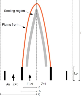
The flame used in this section was studied experimentally by McEnally and Pfefferle [93] for YSI measurements. The burner consists of two concentric tubes, with fuel in the inner tube and air between the inner and outer tube. 0.4 cm of the fuel (and also air) pipe exit is simulated to allow for the fully-development of the velocity profile at the exit of the fuel pipe. Expanding the computational domain inwards the fuel pipe direction has been shown to be important to overcome a numerical error shown by Bennett et al.[110]. The burner configuration is depicted in Fig. 3.1, and the characteristic parameters of the burner and the inlet co-flow are listed in Table3.1. A more detailed description of the burner configuration is given in [111]. The fuel stream velocity profile is taken to be parabolic (i.e. fully-developed laminar profile) based on its mean bulk velocity. On the other hand, the velocity profile in the oxidizer stream is not fully developed and is taken to be flat.
Figure 3.1: Schematic of the diffusion flame and burner configuration.
Pipe inner radiusRi 0.555 cm Full domain radiusR 5.1 cm
Pipe outer radiusRo 0.635 cm Full domain lengthL 20 cm
Burner wall thicknessRo−Ri 0.08 cm Pipe exit lengthLp 0.4 cm
Fuel stream inlet velocity 14.39 cm/s Oxidizer stream inlet velocity 7.03 mm/s Fuel stream inlet temperature 425 K Oxidizer stream inlet temperature 300 K CH4mole fraction in fuel stream 0.55 O2 mole fraction in oxidizer stream 0.21
N2 mole fraction in Fuel 0.45 N2 mole fraction in oxidizer stream 0.79
[image:38.612.240.403.346.539.2]Dopant mole fraction in fuel stream 400ppm
In the simulation, temperatures were under-predicted when the fuel inlet temperature was taken to be 350K [93]. This is consistent with the fact that the burner, as well as the inlet fuel stream, are preheated by heat conduction from the flame and by absorption of heat radiated from the flame region. Unfortunately, the burner wall temperature is not specified in the experiment. Estimating it numerically is beyond the scope of the present work. Gradually increasing the fuel inlet temperature in the simulation is consistent with the intent of searching for the value of the burner exit temperature in the experiment. With a fuel inlet temperature of 425K, the downstream temperature profiles showed better agreement with the experimental data. The fuel inlet velocity is also raised to keep the fuel inlet mass flow rate unchanged. A similar correction (425K instead of 350K) was applied in the simulation of a similar flame by Smookeet al.[89]. The temperature increase from 350K to 425K for fuel stream is physically reasonable, since the temperature on the centerline is measured to be 450K at the position closest to the burner exit (2mm from the exit plane), and an abrupt change in temperature is not expected in this small cold region.
3.1.2
Chemistry model
The detailed chemistry model employed in the current work was developed by Blanquartet al.[3,33]. It contains 185 species and 1903 reactions (forward and backward reactions counted separately) and takes into account all major pathways of PAH formation. This chemical model has been extensively tested and validated in multiple configurations, including laminar premixed flames, laminar diffusion flames, and homogeneous reactors. The chemistry model is provided in the supplemental material of [23].
3.1.3
Numerical set-up
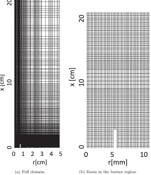
discretization of the computational domain is depicted in the following figure.
0 1 2 3 4 5
0
1
0
20
x
[cm]
r[cm]
(a) Full domain.
0
5
10
r[mm]
0
10
20
x
[cm]
[image:40.612.176.476.109.458.2](b) Zoom in the burner region.
Figure 3.2: Axisymmetric structured mesh used for the flame simulations.
As can be seen in Fig. 3.2, the mesh is non-uniform and most refined near the region where the main chemical reactions and diffusion processes occur (around the burner exit and the flame centerline) and is stretched in both axial and radial directions away from the burner exit to reduce the computational cost. The numerical simulation is shown to give the same results when a 256×128 staggered mesh is used. This will be shown in the budget analysis detailed in Chapter.4.3.3.
of the computational domain shown in Fig. 3.2). The flames simulated in this thesis are co-flow diffusion flame (both laminar and turbulent). The co-flowing oxidizer streams in both the laminar flame simulated in the chapter and the turbulent flame simulated in Chapter. 6 act as a shield to protect the flame from ambient perturbations. Therefore, there is practically no flow entrainment at the sides of the computational domain (left and right boundaries of the computational domain). Accounting for this particular type of set-up, Neumann boundary conditions are imposed for scalar quantities and velocity components in the directions parallel (stream-wise and span-wise) to the sides of the computational domain. The velocity component in the cross-stream direction is set to zero on the sides, given the set-up (co-flowing oxidizer shield) of the simulated flames.
3.1.4
Results
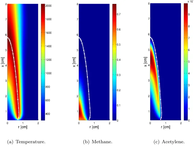
The temperature, methane mass fraction, and acetylene mass fraction fields are depicted in Fig.3.3, Methane and acetylene mass fractions play important roles in determining the local soot yield.
[image:41.612.153.475.402.648.2](a) Temperature. (b) Methane. (c) Acetylene.
Figure 3.3: Temperature, methane mass fraction, and acetylene mass fraction fields from the 2D direct simulation. Dashed lines indicate the location of the stoichiometric surface.
mass fraction indicates the location of PAH formation and the intensity of soot particle surface growth.
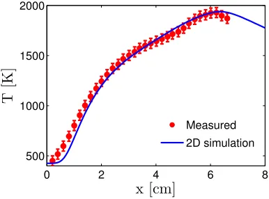
Figure3.4shows a comparison of the centerline temperature profile with the experimental data, and only minor differences may be observed.
0 2 4 6 8
500 1000 1500 2000
x [cm]
T
[K
]
Measured
[image:42.612.218.411.176.319.2]2D simulation
Figure 3.4: Centerline gas temperature.
First, the slope of the calculated temperature profile at the burner exit is practically zero, whereas the experimental data shows a relatively strong gradient right at the burner exit on the centerline. While a finite temperature gradient is expected at the burner wall due to heat conduction, it is unlikely that such gradient would be found at the centerline. This gradient might be related to measurement uncertainties, since it is hard to measure this small cold region inside a hot flame by using a probe with finite size (thermocouple). Second, in the highly sooting region (z= 40−50mm), the measured temperature is slightly lower than the calculated temperature. This may result from heat losses due to radiation of soot particles, which is not included in the current model. In any case, these differences remain very small and are well within the experimental uncertainties.
tendencies using 2D simulation data.
3.2
Conventional laminar diffusion flamelet results
The simulation presented in the previous section is computationally expensive, since all species transport equations are solved simultaneously with the Navier-Stokes equations. Predicting YSIs using direct simulations is even more costly, since a different simulation needs to be carried out for the flame doped with each test hydrocarbon. Therefore, a computationally more efficient approach is required to compute numerically YSIs.
Based on these considerations, one natural approach to calculate numerically YSI is to use a flamelet-based model [49, 50], since the one-dimensionality of the flame structure predicted by the flamelet model can be applied to the (one-dimensional) flame centerline.
In this section, calculations using the conventional steady-state Laminar Diffusion Flamelet (LDF) model are performed on the flame centerline, using information extracted from the direct simulation presented in the previous section. The intent is to reproduce species mass fraction pro-files. Consistent with the direct simulation, no soot model is included in the flamelet model.
3.2.1
Laminar diffusion flamelet equations
The LDF model was introduced originally by Peters and derived from the species transport equations (Eq.2.8) combined with the mixture fraction transport equation (Eq.2.6) [49,50]. It assumes that in diffusion flames, combustion takes place essentially in a thin layer close to the flame front, defined as a flamelet. Based on a coordinate transformation, species mass fractions and temperature transport equations can be re-expressed into one-dimensional flamelet equations. The steady-state flamelet equations in the limit of unity Lewis number diffusion can be expressed as
−1 2ρχ
∂2Y
i
In the above equation, the scalar dissipation rate,χ, is defined as
χ= 2D|∇Z|2, (3.2)
where D is the mass (thermal) diffusivity (Eq. 2.7). For non-unity Lewis transport, the flamelet equations become more complex and additional terms are present [112]
1 4
1− 1
Lei
1
ρ ∂ρχ
∂Z +ρχ
cp λ
∂ ∂Z
λ
cp
∂Y
i
∂Z −
1 2Leiρχ
∂2Y
i
∂Z2 = ˙ωi. (3.3)
In the above equations, the terms which accounts for gradients in the mixture molecular weight and ensures zero net diffusion flux are not shown for clarity. The reader is referred to [112] for the full version and a complete derivation of these equations for non-unity Lewis number diffusion, under flat and thin flame assumptions. The above equation is a second-order ordinary differential equation in mixture fraction space, since all variables in the above equations are only functions of mixture fraction [112]. Solving these flamelet equations is equivalent to solving a boundary value Problem.
Most existing simulations of diffusion flames with the flamelet model are based on a simplifying assumption of unity Lewis number [15, 42, 22]. While this assumption may be valid for turbulent flames [63, 113], it is questionable to apply it to laminar flames. In the simulations conducted in this work, a unity Lewis number was not assumed and a constant, non-unity Lewis number was calculated for each species. Therefore, differential diffusion effects are included. In the present work, these equations (Eq. 3.3) are solved using the FlameMaster code [103]. Details about the FlameMaster code is provided in Appendix.E.
3.2.2
Results
0 0.2 0.4 0.6 0.8 1 0 0.1 0.2 0.3 0.4 0.5 0.6 0.7 0.8 Z χ [1 / s]
(a) Scalar dissipation rate.
0 0.2 0.4 0.6 0.8 1
0 500 1000 1500 2000 Z T [K ] (b) Temperature.
0 0.2 0.4 0.6 0.8 1
−25 −20 −15 −10 −5 0 Z u ∂
Z[∂x
s
−
1]
Flamelet
2D simulation
(c) Axial velocityu∂Z∂x.
Figure 3.5: Scalar dissipation rate, temperature, and axial velocity profiles extracted from the 2D simulation along the centerline plotted in mixture fraction space.
simulation results on the centerline using the following expression
χ= 2D
∂Z ∂x 2 , (3.4)
since the derivative ofZin the radial direction vanishes thanks to axisymmetry. The extracted scalar dissipation profile is fitted and imposed in the flamelet calculations, as shown in Fig.3.5(a). Second, the centerline temperature profile is also extracted and imposed (Fig.3.5(b)), instead of solving the corresponding flamelet equation for temperature (Similar to Eq.3.3). Although imposing the tem-perature profile is not strictly necessary, it is more consistent than solving it directly since unsteady radiation heat losses (Eq.2.5) are not compatible with the steady-state flamelet equation [15].
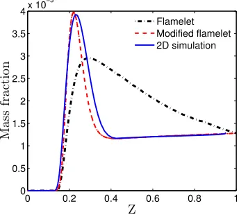
The resulting mass fraction profiles for several representative species are depicted in Fig. 3.6. The locations of maximum species mass fraction are not well predicted by the flamelet model as they are on the richer side of the mixture compared to those predicted by the direct simulation. Furthermore, mass fraction profiles predicted by the flamelet model show an approximately linear decrease in mixture fraction space from the locations of maximum values on the rich side of the mixture, suggesting that diffusion is predominant compared to convection at large mixture fractions. On the contrary, results from the direct simulation indicate that species are strongly convected from the fuel inlet (Z = 1) towards the lean side before getting diffused.
0 0.2 0.4 0.6 0.8 1 0 0.002 0.004 0.006 0.008 0.01 Z M a s s fr a c t io n Flamelet 2D simulation
(a) C2H2.
0 0.2 0.4 0.6 0.8 1
0 1 2 3 4 5 6 7 8x 10
−4 Z M a s s fr a c t io n Flamelet 2D simulation
(b) P-C3H4.
0 0.2 0.4 0.6 0.8 1
0 0.5 1 1.5 2 2.5 3 3.5
4x 10
−3 Z M a s s fr a c t io n Flamelet 2D simulation
(c) C6H6.
Figure 3.6: Comparison of species mass fraction in mixture fraction space between the DNS and the conventional flamelet model.
a convective term in mixture fraction, u∂Z ∂x
∂Y
∂Z, with convection velocityu ∂Z
∂x. Using the balance
between convection and diffusion in the mixture fraction transport equation, this term is computed as u∂Z ∂x = 1 4 1 ρ ∂ρχ
∂Z +ρχ
cp λ ∂ ∂Z λ cp , (3.5)
in the conventional flamelet model [112] (Eq. 3.3). As will be shown in the next section, this expression underestimates significantly the actual convective effect (Fig.3.5(c)). These discrepancies demonstrate that the flamelet model fails to capture the correct dominant physical processes for mixture fractions beyond the stoichiometric value. These rich conditions are of critical importance for the formation of Polycyclic Aromatic Hydrocarbons (PAH). Hence, a new numerical framework is required to reproduce the correct physics along the centerline, where thin flamelet hypothesis may not be valid.
3.3
Derivation of modified flamelet equations
is due to the fact that YSI are defined as functions of the maximum soot volume fraction on the centerline. Consequently, it is sufficient to derive and solve diffusion flamelet equations that are only valid on the centerline. Further, modeling the flame centerline as a single flamelet is feasible since the value of the mixture fraction variable goes from one at the fuel burner surface, to practically zero at elevated flame heights above the burner exit plane. Modified flamelet equations are derived from the continuity equation (Eq.2.1) and the species transport equations (Eq.2.8).
3.3.1
Preliminary considerations
Under thin flame assumptions, the conventional flamelet model [112] assumes that all variables are only functions of the mixture fraction. It is further assumed that all derivatives along the flame front are negligible when compared to derivatives across the flame [49, 50]. This may not be valid for a co-flow diffusion flame along the centerline, where the characteristic length scale in the radial direction (across the flame) is not negligible compared to the axial length scale (along the flame). Based on the above concern, mapping all physical variables only in the one-dimensional mixture fraction space might not be sufficient to capture multi-dimensional convection and diffusion effects.
3.3.2
New mapping
A new mapping parameter φ, whose gradient lies in the local iso-surface of mixture fraction is introduced, with
∇Z(x, r)· ∇φ(x, r) = 0. (3.6)
With this new variable, a coordinate change is performed between the cylindrical variables (r, x) and the phase space variables (Z, φ). Consequently, derivatives in physical space can be expressed as
∂
∂x =
∂Z ∂x
∂
∂Z +
∂φ ∂x
∂
∂φ, (3.7)
∂
∂r =
∂Z ∂r
∂
∂Z +
∂φ ∂r
∂
According to axisymmetry, the boundary conditions on the centerline are
v|r=0= 0, ∂Z
∂r|r=0= 0, ∂Yi
∂r|r=0= 0, (3.9)
where v is the velocity component in the radial direction. To ensure orthogonality between the gradient ofZ andφ, the latter must satisfy
∂φ
∂x|r=0= 0 (3.10)
on the centerline. In other words, φis constant along the centerline. It will be assume to be zero without loss of generality. The equations listed above lead to the following modified flamelet equation
1− 1
Lei
u∂Z
∂x ∂Yi
∂Z =
1 2
χ Lei
∂2Y
i
∂Z2 +
1 2
ξ Lei
∂2Y
i
∂φ2 +
˙
ωi
ρ, (3.11)
where
ξ= 2D|∇φ|2, (3.12)
anduis the velocity component in the axial direction along the centerline. The terms corresponding to molar diffusion, mass correction diffusion, and molar correction diffusion are included in the derivation, but not shown in the above equation for clarity.
In the above equation, the species mass fractions are functions of the two phase space variables
Z and φ, Yi(Z, φ). The dissipation rates of Z (i.e. χ) and φ (i.e. ξ) are evaluated from the 2D
3.3.3
Effects of the different terms
The modified flamelet equation represents the balance between convection, diffusion, and chemistry in mixture fraction space, with a convective velocity given by (Fig.3.5(c))
uz=u
∂Z
∂x. (3.13)
This convective velocity is in phase space (mixture fraction space), not in physical space. Therefore, the unit ofuzis notm/sbut 1/s, since the mixture fraction variable does not have any dimension.
It is interesting to note that the convective term in the mixture fraction space disappears if the Lewis number is unity. This underlines the importance of differential diffusion effects for this particular flame. It also shows that heavier species (such as PAH) will be more affected by non-unity Lewis number effects.
The mass diffusion term 12Leχi∂2Yi
∂Z2 appears in both the conventional and modified flamelet
equa-tions, representing diffusion in the direction orthogonal to the local iso-surface of mixture fraction. The additional mass diffusion term 1
2
ξ Lei
∂2Yi
∂φ2 in Eq.3.11represents diffusion in the direction parallel
to the local iso-surface of mixture fraction, which is neglected by the conventional flamelet model. This term is able to redistribute the species in a way that is depicted in Fig.3.7.
ϕ Iso-surface Z Iso-surface
Diffusion in ϕ Diffusion in Z
Effective diffusion in Z
Figure 3.7: Schematic of the diffusion process. The dashed lines represent the mixture fraction iso-contours, and the dash-dot lines representφiso-contours.
3.3.4
Closure of the modified flamelet equations
and 3.2). In other words, the modified flamelet equations (Eq. 3.11) are not closed in mixture fraction space, as the parameterφis independent of the mixture fraction (Eq.3.6).
In the current work, in order not to obviate the distinct advantage offered by the flamelet model, both diffusion terms inZ andφare combined into one single term by introducing a new parameter
χ0 as the aggregate scalar dissipation rate. Mathematically, this means
1 2
χ Lei
∂2Y
i
∂Z2 +
1 2
ξ Lei
∂2Y
i
∂φ2 =
1 2
χ0 Lei
∂2Y
i
∂Z2. (3.14)
Obviously, the above equation is not valid everywhere in the domain, and it is valid and considered only on the flame centerline. Physically, this treatment is equivalent to representing the diffusion path directed by the arrows outside the flame axis by the diffusion arrow on the flame axis, as shown in Fig.3.7. This yields the resulting balance equation
1− 1
Lei
uz
∂Yi
∂Z =
1 2
χ0 Lei
∂2Y
i
∂Z2 +
˙
ωi
ρ. (3.15)
As mentioned previously, additional terms accounting for molar/mass diffusion and ensuring z