Loop
.
White Rose Research Online URL for this paper:
http://eprints.whiterose.ac.uk/106776/
Version: Accepted Version
Article:
Al-Ghafri, K.S. and Erdélyi, R. (2013) Effect of Variable Background on an Oscillating Hot
Coronal Loop. Solar Physics, 283 (2). pp. 413-428. ISSN 0038-0938
https://doi.org/10.1007/s11207-013-0225-8
Reuse
Unless indicated otherwise, fulltext items are protected by copyright with all rights reserved. The copyright exception in section 29 of the Copyright, Designs and Patents Act 1988 allows the making of a single copy solely for the purpose of non-commercial research or private study within the limits of fair dealing. The publisher or other rights-holder may allow further reproduction and re-use of this version - refer to the White Rose Research Online record for this item. Where records identify the publisher as the copyright holder, users can verify any specific terms of use on the publisher’s website.
Takedown
arXiv:1203.6765v1 [astro-ph.SR] 30 Mar 2012
DOI: 10.1007/•••••-•••-•••-••••-•
The Effect of Variable Background on Oscillating Hot Coronal Loop due to
Thermal Conduction
K.S. Al-Ghafri and R. Erd´elyi
c
Springer••••
AbstractWe investigate the effect of a variable,i.e.time-dependent, background on the standing acoustic
(i.e.longitudinal) modes generated in a hot coronal loop. A theoretical model of 1D geometry describing
the coronal loop is applied. The background temperature is allowed to change as a function of time and undergoes an exponential decay with characteristic cooling times typical for coronal loops. The magnetic field is assumed to be uniform. Thermal conduction is the dominant mechanism of cooling the hot background plasma in the presence of an unspecified thermodynamic source that maintains the initial equilibrium. The influence of the rapidly cooling background plasma on the behaviour of standing acoustic (longitudinal) waves is investigated analytically. The temporally evolving dispersion relation and wave amplitude are derived by using the WKB theory. An analytic solution for the time-dependent amplitude that describes the influence of thermal conduction on the standing longitudinal (acoustic) wave is obtained by exploiting the properties of Sturm-Liouville problems. Next, numerical evaluations further illustrate the behaviour of the standing acoustic waves in a system with variable, time dependent background. The results are applied to a number of detected loop oscillations. We find a remarkable agreement between the theoretical predictions and the observations. The cooling of the background plasma due to thermal conduction is found to cause a strong damping for the slow standing magneto-acoustic waves in hot coronal loops in general. Further to this, the increase in the value of thermal conductivity leads to a strong decay in the amplitude of the longitudinal standing slow MHD waves.
Keywords: Magnetohydrodynamics(MHD)·Plasmas·Sun: corona·Waves
1. Introduction
Recent consecutive solar observations by high-resolution imaging space telescopes and spectrometers have shown that the solar atmosphere is dynamic in nature and is composed of numerous magnetic structures of which coronal loops are of the centre of focus in this paper. It has been confirmed that these complex struc-tures of the solar corona can support a wide range of magnetohydrodynamic (MHD) waves which are nat-ural carriers of energy and may have the key to solve the problem of solar coronal heating (see, the recent
review bye.g.Taroyan and Erd´elyi, 2009; McLaughlinet al., 2011). In particular, one MHD wave mode
present in coronal loops has become the centre of attention: the slow magneto-acoustic mode. The slow (propagating and standing) MHD waves are extensively supported by the solar coronal structures and are
observed to be rapidly damped (Wanget al., 2003a; Wanget al., 2003b; De Moortel, 2009; Wang, 2011).
Propagating intensity disturbances were first detected by the Ultraviolet Coronagraph Spectrometer
onboard the Solar Heliospheric Observatory(SOHO/UVCS) along coronal plumes (Ofmanet al., 1997;
Ofman et al., 1999; Ofmanet al., 2000a), and were identified as slow magneto-acoustic waves (Ofmanet al., 1999).
Subsequently, similar intensity disturbances were observed in coronal loops by the Transition Region
Solar Physics and Space Plasma Research Centre (SP2
RC), University of Sheffield, Hicks Building, Hounsfield Road, Sheffield S3 7RH, UK
e-mail:[email protected]
and Coronal Explorer(TRACE) (Nightingaleet al., 1999; Schrijveret al., 1999; De Moortelet al., 2000;
McEwan and De Moortel, 2006) and the EUV Imaging Telescope onboard theSolar Heliospheric
Obser-vatory(SOHO/EIT) (Berghmans and Clette, 1999). Nakariakovet al.(2000) found that the slow MHD wave evolution is affected by dissipation and gravitational stratification. Erd´elyi and Taroyan (2008) and Wang et al.(2009) have detected longitudinally propagating slow MHD waves with around five-minute
period in the transition region and five coronal lines at the footpoint of a coronal loop by Hinode/EIS.
The source of these oscillations are suggested to be the leakage of the pmodes from photosphere region
through the chromosphere and transition region into the corona (De Pontieuet al., 2005).
Oscillations interpreted as longitudinal standing (slow) magneto-acoustic waves have been observed
in hot (T > 6 MK) active region loops by the Solar Ultraviolet Measurement of Emitted Radiation
(SUMER) spectrometer on board SOHO (Wanget al., 2002; Wanget al., 2003b; Taroyanet al., 2007).
These oscillations have periods in the range of 8.6 to 32.3 minutes with decay times of 3.1−42.3
minutes and amplitudes between 12 and 353 km s−1
(Wanget al., 2005). Moreover, Mariska (2005)
have reported Doppler shift oscillations during solar flares with Yohkoh in a high temperature region
reaching 12−14 MK. These oscillations are interpreted in terms of the standing-slow mode MHD waves
(Mariska, 2006). Evidence for the standing slow mode can be underpinned from the phase relationship between velocity and intensity where a quarter-period phase difference is a characteristic of the standing waves while the propagating waves exhibit an in-phase relationship. Therefore, an approximate quarter-period delay of the intensity variations behind the Doppler shift strongly support that the oscillations observed by SUMER are slow standing modes. The observed oscillations in coronal loops indicate that the standing slow modes are likely triggered by micro-flares which are produced by impulsive heating
(Mendoza-Brice˜noet al., 2002). In a recent work, Taroyan and Bradshaw (2008) found that longitudinal
standing waves can be excited in cooler EUV loops under the effect of all important mechanisms such as gravitational and thermal stratification, losses, etc. According to this study, hot loops are not only the origin of the standing waves but these waves can also be formed in cooler loops.
Nowadays, the damping of slow magneto-acoustic waves have become a subject of remarkable obser-vational and theoretical attention due to a possibility of damping timescale of the waves on disclosing the physical processes that dominate the energy of the coronal loop in which they are detected. The majority of theoretical and numerical studies on damping of propagating and standing slow MHD waves show that the understanding of dominant mechanisms of rapid damping can be captured from 1D
linear (Sigalottiet al., 2007) or nonlinear model (Wang, 2011). For instance, Ofman and Wang (2002)
and Mendoza-Brice˜noet al.(2004) found that the standing MHD waves are strongly damped because of
thermal conduction in nonlinear model whereas using a linear MHD model Pandey and Dwivedi (2006) indicated that the individual influence of thermal conduction or viscosity is not enough to account for the observed damping. In a static 1D isothermal medium, De Moortel and Hood (2003) investigated the behaviour of both propagating and standing slow MHD waves in the presence of thermal conduction and compressive viscosity. They found that thermal conduction is the dominant damping mechanism of thermal and magneto–acoustic waves in coronal loops. It is also shown that thermal mode is damped in
the form of standing waves. Moreover, Mortonet al.(2010) have shown that the radiative cooling causes
a damping of the slow mode by up to 60% within characteristic lifetimes.
Mendoza-Brice˜noet al.(2004) studied the influence of gravitational stratification on damping of
stand-ing MHD waves in hot coronal loops and found that enhanced nonlinear viscous dissipation due to gravity
may reduce the damping times by about 10−20% compared to the unstratified loops. In contrast to
most recent work, Sigalottiet al.(2007) found that thermal conduction can only be accounted as damping
mechanism when the compressive viscosity is added to the model. Bradshaw and Erd´elyi (2008) reported that the radiation due to a non-equilibrium ionisation balance could cause by up to 10% reduction of
wave-damping timescale in comparison to the equilibrium case. Verwichteet al.(2008) showed that shock
dissipation at large amplitudes gives rise to enhancement of the damping rate which is up to 50% larger than given by thermal conduction alone. In non-isothermal, hot, gravitationally stratified coronal loops,
Erd´elyiet al. (2008) investigated the damping of standing slow (longitudinal) waves and found that the
of second-order scaling polynomial. In all these earlier studies the background (equilibrium) plasma was considered time-independent. This is certainly a working model as long as the background plasma changes occur on timescales much longer than typical perturbation timescales. In a recent theoretical work by
Erd´elyiet al.(2011), the cooling of the background plasma due to thermal conduction has been found to
decreasethe rate of damping of the propagating magneto–acoustic waves in a weakly stratified atmosphere where temporal changes in the slowly evolving equilibrium were considered.
In this study, we examine how the cooling background state affects the longitudinalstandingwaves in
a uniform magnetised plasma. The additional complexity of a time-dependent background gives us a step along to model hot coronal loops. The cooling of the background plasma is assumed to be dominated by thermal conduction in the presence of an unspecified thermodynamic source where the plasma is assumed to be cooling in time with an exponential profile. The coefficient of thermal conductivity is presumed to be varying as a function of time to investigate how the variation of thermal conduction influences the behaviour of standing slow-mode waves. The geometry of coronal loop is described by a semi-circular shape. An analytical solution for the time-dependant amplitude of the standing slow MHD waves is derived using the WKB theory with the aid of properties of Sturm-Liouville problems. The results exhibit that thermal conduction causes a significant variation on the amplitude of the standing magneto–acoustic modes with time. The amplitude of waves are found to suffer damping due to the cooling of the background plasma by thermal conduction. The influence of the ratio change of the period of standing oscillation to the cooling time scale on the rate of damping of hot-loop oscillations seems to be highly efficient, where increasing the value of this ratio deceases the strength of damping rapidly.
2. The Model and Governing Equations
Consider a uniformly magnetised plasma in which the temperature is changing as a function of time due to thermal conduction and the density is a constant. The magnetic field is assumed to be uniform and
[image:4.595.89.538.382.469.2]aligned thez-axes,i.e. B0=B0ˆz. Therefore, the background state can be described as follows:
Figure 1.: Coronal loop
T0=T0(t), (1)
p0=p0(t), (2)
ρ0= const., (3)
B0= const., (4)
ǫ= P τc ≪
1. (5)
Here T0,p0,ρ0andB0are the background quantities identifying the temperature, pressure, density and
magnetic field, respectively; andP is the period of the loop oscillation andτc is the cooling time scale.
The governing MHD equations for the background plasma take the following form
∂ρ
∂t +∇.(ρv) = 0, (6)
ρ∂v
∂t +ρ(v.∇)v=−∇p+ 1 µ0
(∇ ×B)×B, (7)
R ˜ µρ
γ
∂ ∂t
T
ργ−1+ (v.∇)
T ργ−1
= (γ−1)∇(κk∇T) +L, (8)
p=R ˜
µρT, (9)
∂B
where v is the flow velocity, B is the magnetic field, g is the gravity,µ0 is the magnetic permeability
of free space, γ is the ratio of specific heats,R is the gas constant, ˜µ is the mean molecular weight, T
is the temperature, ∇(κk∇T) is the thermal conduction term whereκk =κ0T5/2, L is an unspecified
thermodynamic source term,ρandpare the plasma density and its pressure, respectively.
Assuming that there is no background flow and the background density is constant, so the previous equations determining the background plasma state reduce to
v0= 0, ρ0= const., (11)
∇p0= 0, (12)
p0=
R ˜
µρ0T0, i.e. p0∼T0, (13)
R ˜ µρ0
dT0
dt =L, (14)
where the 0 index denotes background quantity. The observed cooling of coronal loops has been shown to be well-approximated by exponential profile for radiative-cooling loops (Aschwanden and Terradas,
2008; Morton and Erd´elyi, 2009, 2010). More recently, Erd´elyiet al. (2011) found that the temperature
decreases exponentially in time due to thermal conduction in hot coronal loops. As a result, we will assume here that the cooling temperature profile of coronal loops has the form
T0=T0iexp(− t τc
), (15)
whereT0i is the initial temperature att= 0.
Let us perturb the background state, where all variables can be written in the form
f(z, t) =f0(t) +f1(z, t),
where the subscript 0 refers to the equilibrium quantities and the subscript 1 indicates the perturbed
quantities. In this study we consider longitudinal motions only, i.e. v=vˆz, so the linearised perturbed
MHD equations in a 1D system are
∂ρ1
∂t +ρ0 ∂v1
∂z = 0, (16)
ρ0
∂v1
∂t =− ∂p1
∂z, (17)
R ˜ µ
ρ1
dT0
dt +ρ0
∂T1
∂t + (γ−1)ρ0T0 ∂v1
∂z
= (γ−1)κ0T 5/2 0
∂2
T1
∂z2 , (18)
p1=
R ˜
µ{ρ0T1+T0ρ1}. (19)
Here v1≡v1z is the longitudinal velocity perturbation. It is clear that there are no terms exhibiting the
magnetic field but the standing waves are still guided by the magnetic field. Non-dimensionalisation will
be used to simplify the 1D governing Equations (16)−(19). The dimensionless quantities are introduced
as
˜ t= t
P, z˜= z
L, csi= L
P, p˜0= p0
p0i
, T˜0=
T0
T0i ,
c2
si= γp0i
ρ0
, ρ˜1=
ρ1
ρ0
, p˜1=
p1
p0i
, T˜1=
T1
T0i
, ˜v1=
v1
csi
, (20)
where the subscript i represents the value of the quantity at t= 0,L is the loop length, and csi is the
Now, we aim to find the governing equation for the perturbed velocity, which leads to reveal the behaviour of the standing magneto–acoustic mode subject to initial conditions generated in a hot coronal loop. Using the continuity and ideal gas law equations, Equation (18) in terms of dimensionless variables, removing the tilde for the sake of simplicity, takes the following form
∂2
v1
∂t2 −T0
∂2
v1
∂z2 =
−σ
γ T
5/2 0
∂3
T1
∂z3 , σ=
(γ−1)˜µκ0T 5/2 0i RL√γ p0iρ0
, (21)
where σ is defined as thermal ratio and found to be a small quantity under typical coronal conditions
(see,e.g. De Moortel and Hood, 2003) demonstrated here as
T0= 6×10 5
−5×10⁶
K, ρ0= 1.67×10−
12
kg m−3
, κk= 10−11T
5/2
0 W m
−1
deg−1
, ˜
µ= 0.6, R= 8.3×10³
m2
s−2
deg−1
, γ= 5/3,
L= 108
m,
(22)
giving characteristic values ofσ∈[0.0068,0.48] forT ∈[6×10⁵
,5×106
] in K. Equation (21) with the aid of Equations (12), (13) and (19) will be
1 T07/2
∂2
v1
∂t2 −T0
∂2
v1
∂z2
= −σ
γ ∂3
∂z3
p
1
T0 −
ρ1
. (23)
Differentiating with respect to time and, using Equations (16) and (17), we obtain
∂ ∂t
"
1 T07/2
∂2
v1
∂t2 −T0
∂2 v1 ∂z2 # = σ γ γ T0 ∂4 v1
∂t2∂z2 +γ
d dt(
1 T0
)∂
3
v1
∂t∂z2 −
∂4
v1
∂z4
, (24)
which is the governing equation and can be recast to a convenient form for further analysis:
∂ ∂t
∂2
v1
∂t2 −T0
∂2 v1 ∂z2 = 7 2 1 T0
dT0
dt
∂2
v1
∂t2 −T0
∂2
v1
∂z2
−σT03/2
dT0
dt ∂3
v1
∂t∂z2+σT 5/2 0
∂2
∂z2
∂2
v1
∂t2 −
T0 γ ∂2 v1 ∂z2 . (25) There are three different cases with interest for the present context one can recover from Equation (25):
Case I. In the absence of the thermal conduction,σ, and the unspecified thermodynamic source in the
energy equation,L ∝ dT0/dt, the governing equation reduces to
∂2
v1
∂t2 −c 2
s ∂2
v1
∂z2 = 0, cs=
p
T0= const., (26)
which has the solution
v1(z, t) =αcos(πz) cos(πcst), (27)
under the boundary conditions representing a line-tied flux tube perturbed as a semi-circular initial motion proportional to its fundamental mode
v1(t,±
1
2) = 0, v1(0, z) =αcos(πz), ∂v1
∂t (0, z) = 0, (28)
where α is the initial amplitude of the standing wave att = 0. A more general, e.g. broad-band,
Case II. In the case of no thermal conduction,i.e.σ= 0, the effect of unspecified thermodynamic source in the system will be found by solving the following equation
∂2
v1
∂t2 −c 2
s ∂2
v1
∂z2 = 0, cs(t) =
p
T0(t)6= const., (29)
which isformally exactly Equation (26) but with variable background temperature,T0 =T0(t). In
spite of the absence of σ, the coefficient of the bracket in the first term in the right-hand-side of
Equation (25) is originally derived from thermal conduction term as seen in Equation (23). Therefore, this term is not added to Equation (29).
Case III. The effect of thermal conduction on the behaviour of the standing acoustic waves in the presence of an unspecified thermodynamic source will be investigated by solving Equation (25).
3. Analytical Solutions
Our goal now is to find an analytic solution to the governing Equation (29) first in case II and next to Equation (25) in case III. Let us point out that Equations (25) and (29) have derivatives multiplied by
small factorsσandǫso this enables the use of the WKB theory to obtain an approximate solution, where
the WKB estimates give good approximations when the smaller value of factor used.
Case II. Let us first start to solve Equation (29) to establish the behaviour of standing magneto– acoustic waves under the influence of an unspecified thermodynamic source in a cooling background state.
Assuming thatt1=ǫtwhich is defined as a slow timescale, meaning the cooling timescale is (much) longer
than the period of the oscillations, Equation (29) will reduce to
∂2
v1
∂t2 1
−c
2
s ǫ2
∂2
v1
∂z2 = 0. (30)
In line with applying the WKB estimates let the perturbed velocity variable have the form
v1(z, t1) =Q(z, t1) exp
i
ǫΘ(t1)
. (31)
The amplitude Qcan be expanded in the power series as follows
Q(z, t1) =Q0+ǫ Q1+· · ·. (32)
Substituting Equations (31) and (32) into Equation (30), and taking terms of order ǫ−3
we obtain at leading order
∂2
Q0
∂z2 +
ω2
c2
s
Q0= 0, (33)
whereω= dΘ/dt1. The boundary conditions (28) applicable to the functionQ0 is
Q0= 0 at z=±
1
2. (34)
Equations (33) and (34) represent a boundary-value problem that determines the frequency of the standing longitudinal (acoustic) mode in a cooling plasma with a varying temperature as function of time. The general solution physically acceptable to this boundary value problem has the form
Q0(z, t1) =
∞
X
n=0
Then, collecting terms of orderǫ−2
, we obtain the equation determining the amplitude
∂2
Q1
∂z2 +
ω2
c2
s Q1=
i c2
s dω
dt1
Q0+ 2ω
∂Q0
∂t1
. (36)
It follows from Equation (28) thatQ1 satisfies the boundary conditions
Q1= 0 at z=±
1
2. (37)
The boundary-value problem, Equations (36) and (37), determiningQ1is a Sturm-Liouville problem and
has a solution only when the right-hand-side of Equation (36) satisfies the compatibility condition, which
is the condition that it is orthogonal to Q0 (see, Ruderman, 2011). This condition can be obtained by
multiplying Equation (36) byQ0, integrating with respect tozfrom−1/2 to 1/2 and using the boundary
conditions (37). The compatibility condition is eventually written as
Z 1/2
−1/2
i c2
s
dω dt1
Q2
0+ 2ωQ0
∂Q0
∂t1
dz= 0, (38)
which gives the amplitude of the standing wave in the following form
An(t1) =An(0) exp( t1
4) =An(0)
s
cs(0) cs(t1)
. (39)
The value of constantAn(0) can be found from Equation (35) att1= 0, which is in the form of Fourier
cosine series, using the boundary condition (28). Then, the solution (39), in scaled (i.e.physical) variables,
takes the form
An(t) =α s
cs(0) cs(t)
. (40)
This result describes the variation of a time-dependent amplitude of longitudinal standing waves in a dynamically cooling magnetic flux tube. Apparently, Equation (40) indicates that the cooling (or heating) leads to an amplification (decrease) of loop oscillation.
Case III. Next, the behaviour of the standing wave in a system dominated by thermal conduction will be obtained by solving the governing Equation (25). Similarly, the WKB theory will be used to find
the solution of Equation (25). Let us now introduce two slow variablest1=ǫtandσ=ǫσ˜, so Equation
(25) will be
∂3 v1 ∂t3 1 +7 2 ∂2 v1 ∂t2 1 −c 2 s ǫ2 ∂3 v1
∂t1∂z2 −
˜ σc5
s ∂3
v1
∂t1∂z2 −
˜ σc5 s ∂4 v1 ∂t2 1∂z 2 − 5 2 c2 s ǫ2 ∂2 v1
∂z2 +
˜ σ ǫ2 c7 s γ ∂4 v1
∂z4 = 0, (41)
and the perturbed velocity by the new scaled variables and the WKB approximation is given by Equation
(31). Substituting Equations (31) and (32) into Equation (41), and taking the highest order terms inǫ,
which is againǫ−3
, we obtain
∂2
Q0
∂z2 +
ω2
c2
s
Q0= 0, (42)
with the boundary conditions
Q0= 0 at z=±
1
The solution to this boundary-value problem is given by
Q0(z, t1) =
∞
X
n=0
Bn(t1) cos ((2n+ 1)πz), ωn = (2n+ 1)πcs, n= 0,1,2,· · ·, (44)
whereBn(t1) stands for the amplitude of the longitudinal standing modes and it will be found by taking
the second highest order terms inǫ for Equation (41) and then using the properties of Sturm-Liouville
problems as follows.
The next largest order terms inǫ, of orderǫ−2
, give the following equation
∂2
Q1
∂z2 +
ω2
c2
s Q1=
i ωc2 s (7 2ω 2
+ 3ωdω
dt1
)Q0+ 3ω 2∂Q0
∂t1
+c2
s ∂3
Q0
∂t1∂z2
+ (5 2c
2
s−σω˜
2
c5
s) ∂2
Q0
∂z2 −σ˜
c7 s γ ∂4 Q0 ∂z4 . (45)
It yields from Equation (28) thatQ1 satisfies the boundary conditions
Q1= 0 at z=±
1
2. (46)
Analogous to Equations (36) and (37), this boundary-value problem, Equations (45) and (46), has a so-lution only when the right-hand side of Equation (45) satisfies the compatibility condition. Consequently,
Z 1/2
−1/2
i ωc2 s (7 2ω 2
+ 3ωdω
dt1
)Q2 0+ 3ω
2
Q0
∂Q0
∂t1
+c2
sQ0
∂3
Q0
∂t1∂z2
+ (5
2c
2
s−˜σω
2
c5
s)Q0
∂2
Q0
∂z2
−σ˜c
7
s γQ0
∂4
Q0
∂z4
dz= 0. (47)
Substituting (44) into (47), we obtain the amplitude of standing wave
Bn(t1) =Bn(0) exp 1
4t1+ ˜ σ 5(
γ−1
γ )(2n+ 1)
2
π2
(c5
s−1)
, (48)
which can be re-written in the scaled variables as
Bn(t) =Bn(0) exp ǫ
4t+
σ 5ǫ(
γ−1
γ )(2n+ 1)
2
π2
(c5
s−1)
. (49)
Now, Equation (44), which represents a Fourier cosine series, with the boundary conditions (28) will be
applied to obtain the value of constantsBn(0). Hence, the solution (49) is
Bn(t) =αexp ǫ
4t+
σ 5ǫ(
γ−1
γ )(2n+ 1)
2
π2
(c5
s−1)
, (50)
which reveals the temporal evolution of longitudinal standing-mode amplitude due to thermal conduction
in a temporally variable (cooling or heating) background plasma. Note that, in the limit σ →0, i.e. if
there is no thermal conduction, Equation (50) reduces to Equation (40) which represents the amplitude variation of standing waves generated in a model of merely cooling plasma without non-ideal effects as,
e.g., thermal conduction.
4. Numerical Evaluations
Mortonet al.(2010) and Erd´elyiet al.(2011) have shown that the WKB approximation estimates
The obtained approximate solutions by the WKB theory can be motivated using numerical evaluations to demonstrate a clear view of the behaviour of MHD waves which is analytically found.
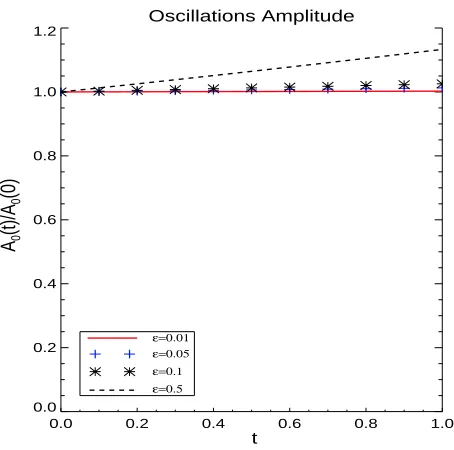
The amplitude of the longitudinal (acoustic) standing waves is plotted after calculating the variables using standard coronal values. Figure 2 shows the variations of the amplitude due to cooling (or heating) mechanism. This graph exhibits an amplification for the wave amplitude caused by the cooling of the
background where increasingǫ (the ratio of the period of oscillation to the cooling time scale) increases
the amplitude. It should be mentioned that this result is in agreement with that reached by Erd´elyiet al.
(2011) who found that the efficiency of damping is reduced by the cooling background plasma, where Figure 2 displays no damping for standing oscillation because the model is purely dominated by the cooling.
Oscillations Amplitude
0.0 0.2 0.4 0.6 0.8 1.0 0.0
0.2 0.4 0.6 0.8 1.0 1.2
A0
(t)/A
0
(0)
t
[image:10.595.186.413.196.421.2]ε=0.01 ε=0.05 ε=0.1 ε=0.5
Figure 2. The amplitude of the standing wave with different values ofǫ(0.01,0.05,0.1,0.5) representing the ratio of period to the cooling time.
Next, in Figure 3 we demonstrate how the amplitude of standing longitudinal (acoustic) waves for a
range of values of ǫand as function of the value of thermal ratio σis changing in different temperature
regions. It is found that the variation of ǫ leads to a considerable change in the rate of damping of
both cool and hot loops. Figure 3a illustrates the trend of amplitude of the EUV (cool) loops such that
the oscillation amplitude decreases slowly in regions of temperature 600,000 K. The decay of the wave
amplitude increases slightly with time in hot corona, for instance loops of temperature 3 MK and 5 MK
as depicted in Figure 3b and 3c, respectively. The strength of damping of hot (e.g.SXT/XRT) loops is
found to be much stronger and shows little change for the smallest values ofǫ, i.e. 0.01−0.1, whereas
large enough values ofǫ, i.e.in the range 0.1< ǫ≤0.5, cause a rapid reduction in the rate of damping
of the wave amplitude. Moreover, it is obvious from Equation (49) that the first term in the exponential function is the same as in Equation (39) were dominated by the cooling. This indicates that the emergence of cooling by thermal conduction in the system of hot coronal loops decreases the rate of damping as exhibited in Figure 3.
In Figure 4 we present the effect of varying the magnitude of thermal conduction coefficient, κ, on
the rate of damping of the standing acoustic wave. Typical values for the coefficient of the thermal
conductivityκ= [10−10
,10−11
,10−12
]T5/2
are taken to shed light on the influence of thermal conduction
Oscillations Amplitude
0.0 0.2 0.4 0.6 0.8 1.0 0.0
0.2 0.4 0.6 0.8 1.0 1.2
(a)
B0
(t)/B
0
(0)
t
ε=0.01 ε=0.05 ε=0.1 ε=0.5
Oscillations Amplitude
0.0 0.2 0.4 0.6 0.8 1.0 0.0
0.2 0.4 0.6 0.8 1.0 1.2
(b)
B0
(t)/B
0
(0)
t
ε=0.01 ε=0.05 ε=0.1 ε=0.5
Oscillations Amplitude
0.0 0.2 0.4 0.6 0.8 1.0 0.0
0.2 0.4 0.6 0.8 1.0 1.2
(c)
B0
(t)/B
0
(0)
t
[image:11.595.192.412.375.599.2]ε=0.01 ε=0.05 ε=0.1 ε=0.5
Figure 3. The amplitude of the standing wave with different values ofǫ(0.01,0.05,0.1,0.5) representing the ratio of period to the cooling time and specific value ofσ,i.e.the value of thermal ratio. (a)σ= 0.0068 (T = 600000 K), (b)σ = 0.17 (T = 3 MK), (c)σ= 0.48 (T = 5 MK).
found that the rate of damping is changing rather rapidly with alteringκby just an order of magnitude
where increasing the value ofκgives rise to a strong decline in the amplitude of the standing slow mode.
Oscillations Amplitude
0.0 0.2 0.4 0.6 0.8 1.0 0.0
0.2 0.4 0.6 0.8 1.0 1.2
B0
(t)/B
0
(0)
t
κ0=10−12
κ0=10−11
κ0=10−10
Figure 4. The amplitude of the standing wave with different values of the thermal-conduction coefficient, κ0=(10−10,10−11,10−12) and specific value of the ratio of period to the cooling time,ǫ= 0.1 whereT = 3 MK.
The significance of the obtained results is to be comparable to observations. We only present here a
2003a), where the standing slow-mode waves are detected only in the region of temperature ≥ 6 MK.
The periods of oscillations are 7−31 minutes. The slow standing wave has seen to be strongly damped
with characteristic decay times 5.7−36.8 minutes mainly likely due to thermal conduction. The typical
length of coronal loops is around 230 Mm.
In our work, we found that hot loop oscillations experience a strong damping due to thermal conduction
which might be comparable with the observed damping provided the value ofǫis small enough as shown
in Figure 3c. Further to this, Figure 4 exhibits that the large value of thermal conduction coefficient leads to a rapid damping which is likely applicable for the observed damping of standing acoustic modes as
discussed by Ofman and Wang (2002) and Mendoza-Brice˜noet al.(2004).
5. Discussion and Conclusion
In this work, we have investigated the influence of a cooling background on the standing magneto-acoustic waves generated in a uniformly magnetised plasma. Thermal conduction is assumed to be the dominant mechanism of cooling background plasma. The background temperature is allowed to change as a function of time and to decay exponentially with characteristic cooling times typical for coronal
loops. The magnetic field is assumed to be constant and in the z direction which may be a suitable
model for loops with large aspect ratio. A theoretical model of 1D geometry describing the coronal loop is applied. A time-dependant governing equation is derived by perturbing the background plasma on a time-scale greater than the period of the oscillation. Three different cases were considered: (I) absence
of thermal conduction σ and unspecified cooling or heating mechanism L, (II) presence of unknown
thermodynamic sourceLonly,i.e.σ= 0, (III) the influence of thermal conductionσcombined with the
unknown mechanismL.
The WKB theory is used to find the analytical solution of the governing equation in case II and III where the governing equation in case I is solved by a direct method and gives the undamped standing
wave,i.e. sound speed is constant. An approximate solution that describes a time-dependant amplitude
of the standing acoustic mode is obtained with the aid of the properties of a Sturm-Liouville problem. The analytically derived solutions are exhibited numerically to give much illustration to the behaviour of MHD slow waves.
In the second case, the individual influence of cooling background plasma on hot-loop oscillation is found to cause an amplification to the amplitude of the longitudinal standing wave. It is noted that the rate of amplification varies according to the change in the ratio of the oscillatory period to the cooling
time scaleǫ, where increasingǫincreases the amplitude of MHD wave.
In the third case, which is of our interest, the temporally dependant amplitude is found to undergo a strong damping due to the cooling of the background plasma by thermal conduction in the hot corona. Further to this, we note that the presence of cooling in a model of hot coronal loop decreases the efficiency
of damping. The variation of the ratio of the period of oscillation to the cooling time scale,ǫ, plays an
effective role on changing the rate of damping of oscillating hot coronal loops, causing a fast decline in the decay degree of oscillation amplitude once the value of this ratio is so large.
The obtained results indicate that this investigation contributes with the previous studies (Morton and Erd´elyi,
2009, 2010; Mortonet al., 2010; Erd´elyiet al., 2011) on demonstrating that the temporal evolution of
coronal plasma due to the dissipative process, i.e. the cooling of the background plasma due to
radia-tion/thermal conduction, has a great influence on the coronal oscillations. In the modelling of solar coronal loop, the temporal and spatial dependant dynamic background plasma is necessary to be considered to understand the properties of observed MHD waves.
References
Aschwanden, M.J., Terradas, J.: 2008,Astrophys. J.686, L127. Berghmans, D., Clette, F.: 1999,Solar Phys.186, 207. Bradshaw, S.J., Erd´elyi, R.: 2008,Astron. Astrophys.483, 301. De Moortel, I.: 2009,Space Sci. Rev.149, 65.
De Moortel, I., Hood, A.W.: 2003,Astron. Astrophys.408, 755.
De Moortel, I., Ireland, J., Walsh, R.W.: 2000,Astron. Astrophys.355, L23. De Pontieu, B., Erd´elyi, R., De Moortel, I.: 2005,Astrophys. J.624, L61. Erd´elyi, R., Taroyan, Y.: 2008,Astron. Astrophys.489, 49.
Erd´elyi, R., Al-Ghafri, K.S., Morton, R.J.: 2011,Solar Phys.272, 73.
Erd´elyi, R., Luna-Cardozo, M., Mendoza-Brice˜no, C.A.: 2008,Solar Phys.252, 305. Mariska, J.T.: 2005,Astrophys. J.620, L67.
Mariska, J.T.: 2006,Astrophys. J.639, 484.
McEwan, M.P., De Moortel, I.: 2006,Astron. Astrophys.448, 763.
McLaughlin, J.A., Hood, A.W., De Moortel, I.: 2011,Space Sci. Rev.158, 205. Mendoza-Brice˜no, C.A., Erd´elyi, R., Sigalotti, L.D.G.: 2002,Astrophys. J.579, L49. Mendoza-Brice˜no, C.A., Erd´elyi, R., Sigalotti, L.D.G.: 2004,Astrophys. J.605, 493. Morton, R., Erd´elyi, R.: 2009,Astrophys. J.707, 750.
Morton, R., Erd´elyi, R.: 2010,Astrophys. J.519, A43.
Morton, R., Hood, A.W., Erd´elyi, R.: 2010,Astron. Astrophys.512, A23.
Nakariakov, V.M., Verwichte, E., Berghmans, D., Robbrecht, E.: 2000,Astron. Astrophys.362, 1151. Nightingale, R.W., Aschwanden, M.J., Hurlburt, N.E.: 1999,Solar Phys.190, 249.
Ofman, L., Wang, T.: 2002,Astrophys. J.580, L85.
Ofman, L., Nakariakov, V.M., DeForest, C.E.: 1999,Astrophys. J.514, 441.
Ofman, L., Romoli, M., Poletto, G., Noci, C., Kohl, J.L.: 1997,Astrophys. J.491, L111. Ofman, L., Romoli, M., Poletto, G., Noci, C., Kohl, J.L. 2000a,Astrophys. J.529, 592. Pandey, V.S., Dwivedi, B.N.: 2006,Solar Phys.236, 127.
Priest, E.R.: 2000,Solar Magneto-hydrodynamics, Kluwer Academic Publishers, 86. Ruderman, M.S.: 2011,Solar Phys.271, 41.
Schrijver, C.J., Title, A.M., Berger, T.E., Fletcher, L., Hurlburt, N.E., Nightingale, R.W., Shine, R.A., Tarbell, T.D., Wolfson, J., Golub, L., Bookbinder, J.A., DeLuca, E.E., McMullen, R.A., Warren, H.P., Kankelborg, C.C., Handy, B.N., De Pontieu, B.: 1999,Solar Phys.187, 261.
Sigalotti, L.D.G., Mendoza-Brice˜no, C.A., Luna-Cardozo, M.: 2007,Solar Phys.246, 187. Taroyan, Y., Bradshaw, S.: 2008,Astron. Astrophys.481, 247.
Taroyan, Y., Erd´elyi, R.: 2009,Space Sci. Rev.149, 229.
Taroyan, Y., Erd´elyi, R., Wang, T.J., Bradshaw, S.J.: 2007,Astrophys. J.659, L173. Verwichte, E., Haynes, M., Arber, T.d., Brady, C.S.: 2008,Astrophys. J.685, 1286. Wang, T.: 2011,Space Sci. Rev.158, 397.
Wang, T.J., Ofman, L., Davila, J.M.: 2009,Astrophys. J.696, 1448.
Wang, T.J., Solanki, S.K., Curdt, W., Innes, D.E., Dammasch, I.E.: 2002,Astrophys. J.574, L101.
Wang, T.J., Solanki, S.K., Curdt, W., Innes, D.E., Dammasch, I.E., Kliem, B. 2003a,Astron. Astrophys.406, 1105. Wang, T.J., Solanki, S.K., Innes, D.E., Curdt, W., E., M. 2003b,Astron. Astrophys.402, 17.