This is a repository copy of
The incorporation of gradient damage models in shell
elements
.
White Rose Research Online URL for this paper:
http://eprints.whiterose.ac.uk/100673/
Version: Accepted Version
Article:
Hosseini, S., Remmers, J.J.C. and De Borst, R. orcid.org/0000-0002-3457-3574 (2014)
The incorporation of gradient damage models in shell elements. International Journal for
Numerical Methods in Engineering, 98 (6). pp. 391-398. ISSN 0029-5981
https://doi.org/10.1002/nme.4640
[email protected] https://eprints.whiterose.ac.uk/
Reuse
Unless indicated otherwise, fulltext items are protected by copyright with all rights reserved. The copyright exception in section 29 of the Copyright, Designs and Patents Act 1988 allows the making of a single copy solely for the purpose of non-commercial research or private study within the limits of fair dealing. The publisher or other rights-holder may allow further reproduction and re-use of this version - refer to the White Rose Research Online record for this item. Where records identify the publisher as the copyright holder, users can verify any specific terms of use on the publisher’s website.
Takedown
If you consider content in White Rose Research Online to be in breach of UK law, please notify us by
Published online in Wiley InterScience (www.interscience.wiley.com). DOI: 10.1002/nme
The incorporation of gradient damage models in shell elements
Saman Hosseini
1, Joris J. C. Remmers
1, Ren´e de Borst
2,∗1Eindhoven University of Technology, Department of Mechanical Engineering, PO BOX 513, 5600 MB, Eindhoven, The
Netherlands.
2University of Glasgow, School of Engineering Rankine Building, Oakfield Avenue, Glasgow G12 8LT, UK.
SUMMARY
An approach is proposed to incorporate gradient-enhanced damage models in shell elements. The approach is elaborated for a solid-like shell element, which is advantageous because of the availability of nodes at the top and bottom shell surfaces, and the presence of a three-dimensional strain state. Some simple examples are given to demonstrate the versatility and the convergence of the method. Copyright c2010 John Wiley & Sons, Ltd.
Received . . .
KEY WORDS: gradient damage models, solid-like shell, composite materials, intralaminar damage
1. INTRODUCTION
The failure behaviour of composite materials is often a combination of multiple damage mechanisms: delamination (interlaminar damage), and matrix cracking and fibre breakage (intralaminar damage). The complex nature of these failure mechanisms requires a reliable computational tool for the prediction of structural integrity.
Microcracks in the matrix are often the first form of damage in laminates. At a mesolevel, where the individual plies of a composite are modelled, matrix cracking can be represented through a continuum damage model [1]. After accumulation of a certain amount of damage, however, continuum damage models lead to ill-posed boundary value problems, which causes a severe mesh dependence [2]. Gradient damage models have been shown to be an efficient solution to this [3].
So far, gradient damage simulations have been restricted to continua, either two or three-dimensional. Structural applications do not seem to have been reported. Bearing in mind that the stresses must be computed accurately for use in intralaminar damage models, solid-like shell elements such as that developed in References [4,5,6] seem to be particularly suitable. Because of the enhanced kinematics a fully three-dimensional stain state exists within the shell, which enables the straightforward use of three-dimensional constitutive relations. The solid-like shell model has another advantage, namely that it carries only translational degrees of freedom. This not only makes it easy to stack them, but, since the translational degrees of freedom are located at the top and bottom surfaces, the associated nodes can also be used for the interpolation of a nonlocal equivalent strain field. Indeed, since in a gradient damage model the nonlocal equivalent strain is interpolated in addition to the displacements, an assumption is required for this additional field as well.
We propose to independently interpolate the nonlocal equivalent strain field at each surface of the shell. In the case of solid-like shell elements the nodes that are needed for this interpolation are
∗Correspondence to: Ren´e de Borst, University of Glasgow, School of Engineering, Rankine Building, Oakfield Avenue,
2 S. HOSSEINI ET AL.
directly available. However, the same procedure can be used for other shell elements, by defining auxiliary nodes that are used for the interpolation of the nonlocal equivalent strain field only. These auxiliary nodes are then obtained from the mid-surface nodes, the local shell director, and the thickness of the shell. With the nonlocal equivalent strain at the top and bottom surfaces at hand, its value anywhere inside the shell can be computed by a linear interpolation between the values at the top and the bottom surfaces, which assumption is consistent with the assumption that straight fibres remain straight.
For completeness we first briefly summarize the gradient damage model and the solid-like shell element. We next show how the gradient damage model can be incorporated in a solid-like shell element. Some simple examples are given to demonstrate the versatility and mesh independence.
2. DAMAGE MODEL
In this paper we assume an isotropic damage model which means that one damage variable, ω, describes the damage process. Herein, the undamaged material is characterized byω= 0and the fully damaged material by ω= 1 (in practice a value close to 1 is used to avoid ill-conditioning of the local stiffness matrix). Assuming small strains, the following relation between the Second Piola-Kirchhoff stress tensorSand the Green-Lagrange strain tensorγis adopted:
S= (1−ω)C:γ (1)
with C the elastic stiffness matrix. In this relation the damage variable is given as:
ω=ω(κ) (2)
with κ a history parameter which retains the most severe deformation. The damage model is completed by a loading functionf as a function of the nonlocal equivalent strainγeq¯ :
f(γ, κ) = ¯γeq(γ)−κ (3)
The history parameter starts at a threshold valueκiand is updated through the Kuhn-Tucker loading-unloading conditions:
f ≤0 , κ˙ ≥0 , fκ˙ = 0 (4)
Following [3] the nonlocal equivalent strainγeq¯ follows from the solution of the partial differential equation:
¯
γeq−c∇
2
¯
γeq=γeq (5)
whereγeq=γeq(γγγ)is the local equivalent strain andcsets the internal length scale.
3. VIRTUAL WORK AND LINEARIZATION
In a Total Lagrangian formulation the principle of virtual work is expressed in the reference configurationΩ0:
Z
Ω0
δγT :SdΩ0=
Z
Γ0
δuTt0dΓ0 (6)
with t0the traction acting on the boundary Γ0 of the initial configuration. Note that neither body
forces nor follower forces have been taken into account. The resulting system of nonlinear equations is typically solved using the Newton-Raphson method, which requires computation of the tangential stiffness matrix. This quantity is obtained by linearizing the internal virtual work, the left side of the equation (6):
D(δWint) = Z
Ω0
δγT :DS + D(δγT) :SdΩ0 (7)
Copyright c2010 John Wiley & Sons, Ltd. Int. J. Numer. Meth. Engng (2010)
Using equation (1) the derivative of the stress tensor is written as:
DS= (1−ω)C:Dγ−∂ω
∂κ ∂κ ∂¯γeq
Dγ¯eqC:γ (8)
where∂κ/∂¯γeq ≡1for loading and∂κ/∂γ¯eq≡0for unloading. Defining
q=∂ω
∂κ
and substituting equation (8) into equation (7) the linearized internal virtual work expression becomes:
D(δWint) = Z
Ω0
δγT : (1−ω)C:Dγ−qDγ¯eqδγT :C:γdΩ0
+ Z
Ω0
D(δγT) :SdΩ0 (9)
where the last term leads to the standard geometric stiffness matrix, which will not be repeated here. Equation (5) is coupled to the equilibrium equation, equation (6), and must be solved concurrently. The variational form of the gradient damage equation is given by:
Z
Ω0
δ¯γeq(¯γeq−c∇2γ¯eq−γeq) dΩ0= 0 (10)
In line with the vast majority of the literature a natural boundary condition is assumed for γ¯eq. Application of the divergence theorem then leads to:
Z
Ω0
(δ¯γeq¯γeq+c∇δγ¯eq· ∇γ¯eq) dΩ0−
Z
Ω0
δ¯γeqγeqdΩ0= 0 (11)
For the derivation of the tangent stiffness matrix this expression must be linearized, leading to:
Z
Ω0
(δ¯γeqD¯γeq+c∇δγ¯eq· ∇Dγ¯eq) dΩ0−
Z
Ω0
δ¯γeqDγeqdΩ0= 0 (12)
where
Dγeq =pTDγ , pT =∂γeq
∂γ (13)
4. SOLID-LIKE SHELL FORMULATION
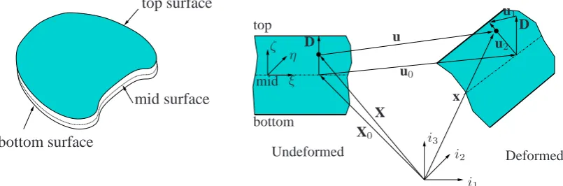
Figure1shows the reference and the current configuration, and the kinematics of the solid-like shell element in curvilinear coordinates. The element kinematics are captured by a linear combination of a pair of material points at the top and at the bottom surfaces of the element. Each point is characterized by a position vector, Xt and Xb for the initial configuration on the top and bottom surfaces, respectively. The variables ξ and η are the local curvilinear coordinates in the two independent in-plane directions, andζis the local curvilinear coordinate in the thickness direction. The position of a material point in the undeformed configuration is written as function of three curvilinear coordinates
X(ξ, η, ζ) =X0(ξ, η) +ζD(ξ, η) (14)
where X0(ξ, η) is the projection of the point on the mid-surface of shell and D is the thickness director in this point:
X0(ξ, η) =1
2[Xt(ξ, η) +Xb(ξ, η)] , D(ξ, η) = 1
4 S. HOSSEINI ET AL.
bottom surface
top surface
mid surface
ξ η ζ D u0 u X X0 x u2 D u1 i1 i2 i3 Deformed Undeformed mid bottom topFigure 1. Geometry and kinematics of the shell in the undeformed and in the deformed configurations.
The position of the material point in the deformed configuration x(ξ, η)is related to X(ξ, η)via the displacement field u(ξ, η, ζ)as:
x(ξ, η, ζ) =X(ξ, η, ζ) +u(ξ, η, ζ) (16)
where
u(ξ, η, ζ) =u0(ξ, η) +ζu1(ξ, η) + (1−ζ2
)u2
(ξ, η) (17)
In this relation, u0
and u1
are the displacements of X0 on the shell mid-surface and the thickness director D, and can be written as:
u0(ξ, η) =1
2[ut(ξ, η) +ub(ξ, η)] , u
1
(ξ, η) =1
2[ut(ξ, η)−ub(ξ, η)] (18)
The internal stretch of the element is represented in equation (17) by the inclusion of a quadratic term in the displacement field, so that the normal strain in the thickness direction varies linearly. u2
is expressed in terms of stretch degrees of freedom,w, as:
u2=w(ξ, η)[D(ξ, η) +u1(ξ, η)] (19)
see also Figure1.
In any material point a local reference triad can be established. The covariant base vectors are then obtained as the partial derivatives of the position vectors with respect to the curvilinear coordinates Θ
Θ
Θ = [ξ, η, ζ]. In the undeformed configuration they are defined as:
Gα= ∂X
∂Θα =Eα+ζD,α , α= 1,2 , G3=D (20)
where(.),αdenotes the partial derivative with respect toΘα. E α= ∂X
0
∂Θα, is the covariant base vector
defined on the mid-surface. Similarly, in the deformed configuration we have:
gα= ∂x
∂Θα =Gα+u
0
,α+ζu
1
,α+ (1−ζ
2
)u2
,α
g3=D+u
1
−2ζu2
(21)
Using equations (20) and (21) the componentsGij andgij of the metric tensors in the undeformed and the deformed configuration, respectively, can be determined as:
Gij =Gi·Gj , gij=gi·gj , i= 1,2,3 (22)
and finally, the representation of the Green-Lagrange strain tensor reads as:
γ=γijGi⊗Gj with γij = 1
2(gij−Gij) (23)
Copyright c2010 John Wiley & Sons, Ltd. Int. J. Numer. Meth. Engng (2010)
From equations (21)–(23) we infer that
γγγ=γγγ(u0,u1,u2) (24)
and using equations (18) and (19):
γγγ=γγγ(ub,ut, w) =γγγ(u, w) (25)
with u= (ub,ut)collecting the displacement degrees of freedom at the bottom and top surfaces. For future use we list the variation of the strain tensor:
δγγγ= ∂γγγ
∂uδu+
∂γγγ
∂wδw (26)
ζ
ξ η
w
¯
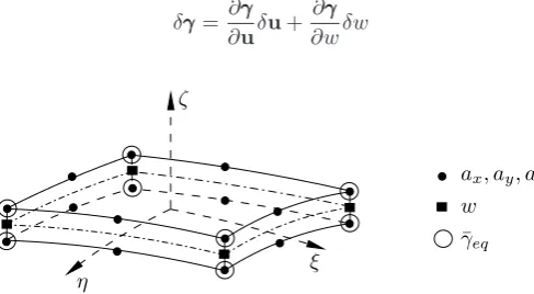
[image:6.595.173.417.176.310.2]γeq ax, ay, az
Figure 2. Geometry of 16 noded solid-like-shell element.
5. FINITE ELEMENT IMPLEMENTATION
In this paper we consider the sixteen-node solid-like shell element, see Figure2. Each node contains three displacement degrees of freedom,ax, ay, az which gives a bi-quadratic interpolation of the in-plane displacement field. With this interpolation for the displacements, the nonlocal equivalent strain fieldγ¯eq should interpolated using bi-linear shape functions to avoid oscillations [7]. Hence, the corner nodes of the solid-like shell element have degrees of freedom for the nonlocal equivalent strain field. It is recalled that the nodes of the top surface are used for the interpolation of the nonlocal equivalent strain field at the top surface, and those of the bottom surface support the nodal parameters of the nonlocal equivalent strain field at the bottom surface. The nonlocal equivalent strain at any point in the shell is then found by an interpolation in the thickness direction of the of the values of the nonlocal equivalent strain at the top and bottom surfaces. The kinematics of the shell are completed by a linear distribution of the internal stretch, which is supported by degrees of freedom located at the four corners of the mid-surface of the element. As detailed in Refs [4,5,6] these are internal degrees of freedom and condensed at element level.
We discretize the displacement, the stretch and the nonlocal equivalent strain as:
u=Hua , w=Hww , γ¯eq =Hγ¯e (27)
where Hu,Hw,Hγ¯contain the corresponding shape functions, and a,w,e are the vectors containing
the degrees of freedom for the displacement, the stretch and the nonlocal equivalent strain, respectively. The strain and the gradient of the nonlocal equivalent strain then become:
γ=Bua+Bww , ∇γ¯eq=Bγ¯e (28)
with Bu,Bw,Bγ¯the matrices that contain the derivatives of the shape functions.
Substituting (27) and (28) for the variational forms in (6) and (11) and requiring that the results hold for arbitrary(δa, δw, δe), the discrete equilibrium equations are obtained as:
Z
Ω0
BTuSdΩ0=
Z
Γ0
6 S. HOSSEINI ET AL.
Z
Ω0
BTwSdΩ0=0 (30)
and averaging equation for the nonlocal equivalent strains becomes:
Z
Ω0
HTγ¯H¯γ+cBTγ¯B¯γ
dΩ0−
Z
Ω0
HT¯γeqγeqdΩ0= 0 (31)
The left-hand sides of equations (29)–(31) leads to the internal force vectors, which can be differentiated to yield the material part of the tangential stiffness matrix:
K=
Kaa Kaw Kae
Kwa Kww Kwe
Kea Kew Kee
(32) where Kaa= Z Ω0
(1−ω)BTuCBudΩ0 Kaw=
Z
Ω0
(1−ω)BTuCBwdΩ0
Kae=
Z
Ω0
qBTuCγeqH¯γdΩ0 Kwa=
Z
Ω0
(1−ω)BTwCBudΩ0
Kww=
Z
Ω0
(1−ω)BTwCBwdΩ0 Kwe=
Z
Ω0
qBTwCγeqHγ¯dΩ0 (33)
Kea=−
Z
Ω0
HT¯γpTBudΩ0 Kew=−
Z
Ω0
HTγ¯pTBwdΩ0
Kee=
Z
Ω0
HT¯γeqH¯γeq+cB
T
¯
γeqBγ¯eq
dΩ0
A2×2Gauss integration rule has been adopted for the in-plane integration for all submatrices, and Cotes integration has been used through the thickness. In the example a five-point Newton-Cotes integration was sufficient.
6. EXAMPLES
We will now assess the implementation of the enhanced gradient damage model by means of two examples.
[image:7.595.99.503.184.385.2]L= 100 mm l= 10 mm
Figure 3. Bar with an imperfection subjected to an axial tension.
6.1. Simulation of continuum damage
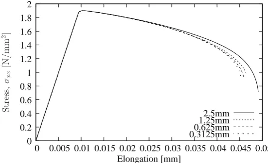
A 3mm thick bar of lengthL= 100mm and of 3.3 mm width (Figure 3) is considered which is subjected to a uniaxial tensile load. To trigger localization the cross sectional area in the centre part of the bar has been reduced by 10% over a lengthl= 10mm. A Young’s modulusE= 2000N/mm2, a fracture energyGc = 0.001N/mm and a tensile strengthft= 2N/mm
2
have been used, together with a linear damage evolution law andc= 1mm2
[3]. The load-displacement graph is shown in Figure4for various levels of mesh refinement. As in previous simulations [3] a proper convergence upon mesh refinement is observed.
Copyright c2010 John Wiley & Sons, Ltd. Int. J. Numer. Meth. Engng (2010)
[image:7.595.196.398.513.566.2]0 0.2 0.4 0.6 0.8 1 1.2 1.4 1.6 1.8 2
0 0.005 0.01 0.015 0.02 0.025 0.03 0.035 0.04 0.045 0.05 Elongation [mm]
2.5mm 1.25mm 0.625mm 0.3125mm
S
tr
es
s,
σxx
[N
/m
m
[image:8.595.159.435.69.237.2]2]
Figure 4. Load-displacement graph of the bar under tension.
6.2. Panel under distributed load
The previous example assesses the convergence for in-plane loadings, but not for a plate that is subject to bending. This is subject of the next example, which is shown in Figure5. The panel has a lengthl= 500mm, a widthb= 250mm, a thicknesst= 10mm, and is clamped on both ends. A Young’s modulusE= 4000N/mm2, a fracture energy Gc= 0.05N/mm and a tensile strength
ft= 2N/mm
2
have been chosen with a linear damage relation andc= 1mm2
. As in the previous example, the simulations have been repeated for different mesh sizes. The results are shown in Figure6, which show a clear mesh independence. Figure7also shows the deformation of the panel and the intensity of the damage evolution.
l= 500 mm
b= 250 mm
t= 10 mm
[image:8.595.162.432.431.511.2]q=sin(πx/l)
Figure 5. Geometry of the panel under sinusoidal traction.
7. CONCLUDING REMARKS
8 S. HOSSEINI ET AL.
0 100 200 300 400 500 600 700
0 1 2 3 4 5
Load [N]
[image:9.595.159.436.67.237.2]Mid−point displacement [mm] 25mm 12.5mm 6.25mm 3.125mm
Figure 6. Load-displacement graph of the panel under sinusoidal traction.
Figure 7. Deformation and damage intensity of the panel.
ACKNOWLEDGEMENTS
Funding from the EU Seventh Framework Programme FP7/2007-2013 under grant agreement n0
213371 (MAAXIMUS, www.maaximus.eu) is gratefully acknowledged.
REFERENCES
1. Ladev`eze P, Lubineau G. An enhanced mesomodel for laminates based on micromechanics. Composites Science and
Technology, 2002;62: 533-541.
2. de Borst R, Crisfield MA, Remmers JJC, Verhoosel CV. Non-linear Finite Element Analysis of Solids and Structures. Wiley Series in Computational Mechanics, Second edition, 2012.
3. Peerlings RHJ, de Borst R, Brekelmans WAM, de Vree HPJ, Gradient-enhanced damage for quasi-brittle materials. International Journal for Numerical Methods in Engineering, 1996; 39: 3391-3403.
4. Parisch H. A continuum-based shell theory for non-linear application. International Journal for Numerical Methods
in Engineering, 1995;38: 1855-1883.
5. Hashagen F, de Borst R. Numerical assessment of delamination in fibre metal laminates. Computer Methods in
Applied Mechanics and Engineering 2000; 185: 141-59.
6. Remmers JJC, Wells GN, de Borst R. A solid-like shell element allowing for arbitrary delaminations. International
Journal for Numerical Methods in Engineering 2003; 58: 2013-2040.
7. Geers MGD, de Borst R, Brekelmans WAM, Peerlings RHJ. Strain-based transient-gradient damage model for failure analyses. Computer Methods in Applied Mechanics and Engineering 1998; 160: 133-153.
Copyright c2010 John Wiley & Sons, Ltd. Int. J. Numer. Meth. Engng (2010)