Research Article
Indoor Massive MIMO Channel Modelling Using
Ray-Launching Simulation
Jialai Weng,
1Xiaoming Tu,
1Zhihua Lai,
2Sana Salous,
3and Jie Zhang
1 1Department of Electrical and Electronics Engineering, University of Sheffield, Sheffield S1 3JD, UK 2Ranplan Wireless Network Design Ltd., Sheffield S1 4DP, UK3Department of Computer Science and Engineering, Durham University, Durham DH1 3LE, UK
Correspondence should be addressed to Jialai Weng; [email protected]
Received 23 January 2014; Revised 1 June 2014; Accepted 1 July 2014; Published 6 August 2014
Academic Editor: Xuefeng Yin
Copyright © 2014 Jialai Weng et al. This is an open access article distributed under the Creative Commons Attribution License, which permits unrestricted use, distribution, and reproduction in any medium, provided the original work is properly cited.
Massive multi-input multioutput (MIMO) is a promising technique for the next generation of wireless communication networks. In this paper, we focus on using the ray-launching based channel simulation to model massive MIMO channels. We propose one deterministic model and one statistical model for indoor massive MIMO channels, both based on ray-launching simulation. We further propose a simplified version for each model to improve computational efficiency. We simulate the models in indoor wireless network deployment environments and compare the simulation results with measurements. Analysis and comparison show that these ray-launching based simulation models are efficient and accurate for massive MIMO channel modelling, especially with application to indoor network planning and optimisation.
1. Introduction
Massive MIMO is to equip a large number of antennas at both the transmitter and the receiver in a wireless communication system. It is also known as large array system. Massive MIMO has the advantage of providing both higher spectral efficiency and power efficiency. Recently, massive MIMO has been widely accepted as a promising technique for the next generation of wireless communication system [1]. See [2,3] for a recent survey on the topic of massive MIMO system.
Site-specific channel modelling is to model the chan-nel using the environment information and physical radio propagation model to obtain the channel information for specific scenarios. Popular site-specific channel models are electromagnetic propagation based methods such as finite-difference time-domain (FDTD) and ray-based methods. One of the major applications for the site-specific channel models is wireless network deployment. The ray-launching algorithm is especially suitable for this application purpose due to the modelling efficiency [4].
Wireless network planning and optimisation is the one of the major applications of the site-specific channel models.
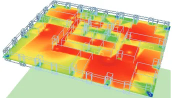
Figure 1 shows a typical channel modelling scenario for indoor network planning. To optimise the locations of the network nodes, such as base station, a large number of potential locations are predicted, which is computationally demanding. Furthermore, large network deployment envi-ronments, such as shopping malls and airports, also pose high computational demands on the prediction model. Therefore, for the application of network deployment and optimisation, a computationally efficient channel model is highly desirable. There have been research works applying the ray-based models to model MIMO channels. The work of [5] is an early research work using ray-tracing to model MIMO channel. The work focused on the limiting factors on channel capacity in MIMO system. Later, the work of [6] proposed to predict MIMO channel using ray-tracing due to its computational efficiency under the setting with a small number of antennas. Moreover the work of [7] studied a similar model focusing on verification of the channel capacity results. This work verified the simulation results with measurements in an indoor scenario with a2 × 2 MIMO system. Furthermore, the work of [8] also studied the MIMO channel matrix based on ray-tracing: not only channel capacity but also various
Figure 1: An example of channel map for indoor network planning.
channel parameters such as angular and delay parameters have also been characterised based on ray-tracing models. As ray-tracing model can provide multipath information, it can be exploited for modelling various channel parameters in multipath channel parameters. So the work of [9] proposed a multipath channel model based on applying ray-tracing model. The MIMO channel parameters have been further derived based on this model. With various MIMO models being proposed, the work of [10] compared the3D ray-tracing MIMO channel models and various statistical models.
The aforementioned research works of ray-based MIMO channel modelling have all focused on modelling the con-ventional MIMO system with a small number of antennas. A ray-based model specifically for massive MIMO system is still missing. Although some of the models can be applied to model massive MIMO channel, the performance, especially the computational efficiency, is unsatisfying to the demand of network planning and optimisation purpose. The primary challenge of modelling massive MIMO channel using ray-based site-specific models, especially for applications in wireless network deployment, is the high computational cost, caused by the large number of antennas.
Another popular site-specific channel modelling tool for network planning is FDTD method and related models [11]. In the application of network planning and optimisation, a large number of channels at different locations over the planning space is computed for optimisation. In such cases, the computational speed of the traditional 3D FDTD model is not satisfying to this requirement of the application. However, purposefully designed and optimised computational efficient models, such as the frequency domain Par-Flow model [12], lack the capability of3D modelling which is essential to the massive MIMO channel.
To address the computational efficiency challenge of modelling massive MIMO channel for wireless network deployment application, we propose to apply a computation-ally efficient intelligent ray-launching algorithm (IRLA) [13] to model massive MIMO system in site-specific scenarios. Its inherent 3D modelling capability and high computational efficiency make it a highly desirable model for network planning and optimisation application.
The purpose of the paper is to propose 2 ray-launching based models in massive MIMO channel modelling for indoor wireless network deployment application. The first ray-launching model is a direct application of ray-launching to massive MIMO modelling. Based on the first model, we further simplified the model by using a reference point. Later we proposed the second model based on probabilistic principle. We also gave a simplified model based on a reference point. These simplified models have the advantage of computational efficiency in massive MIMO modelling. Furthermore, the comparison between the model simulation results and channel measurements shows good agreements.
The organisation of the paper is as follows. In Section2.1
we establish the ray-launching based models for massive MIMO channel. In Section3we present the simulation and measurement scenarios. In Section4.1we analyse and discuss the simulation results. Section5concludes the work.
2. MIMO Modelling Using Ray-Launching
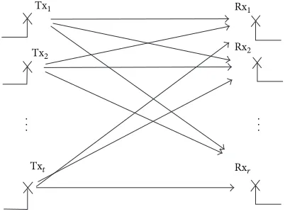
2.1. Deterministic Ray-Launching Model. The MIMO system is to equip multiple antennas both at the transmitter and the receiver. Figure2illustrates a MIMO channel. The transmitter is equipped with a𝑡-element antenna array and the receiver is equipped with an 𝑟-element antenna array. The MIMO channel is then written in the form of matrix as follows:
H=[[[[
[
𝐻1,1 𝐻1,2 ⋅ ⋅ ⋅ 𝐻1,𝑟
𝐻2,1 𝐻2,2 ⋅ ⋅ ⋅ 𝐻2,𝑟
..
. ... d ...
𝐻𝑡,1 𝐻𝑡,2 ⋅ ⋅ ⋅ 𝐻𝑡,𝑟
] ] ] ] ]
. (1)
The matrix element𝐻𝑚,𝑛characterises the channel between the transmitter element 𝑛 and the receiver element 𝑚. In a site-specific channel prediction scenario, the MIMO channel matrix is a function of the locations of the network deployment site. Thus we can write the channel as
H(𝑥, 𝑦, 𝑧, 𝜔) =
[ [ [ [ [ [ [ [ [
𝐻1,1(𝑥, 𝑦, 𝑧, 𝜔) 𝐻1,2(𝑥, 𝑦, 𝑧, 𝜔) ⋅ ⋅ ⋅ 𝐻1,𝑟(𝑥, 𝑦, 𝑧, 𝜔)
𝐻2,1(𝑥, 𝑦, 𝑧, 𝜔) 𝐻2,2(𝑥, 𝑦, 𝑧, 𝜔) ⋅ ⋅ ⋅ 𝐻2,𝑟(𝑥, 𝑦, 𝑧, 𝜔)
..
. ... d ...
𝐻𝑡,1(𝑥, 𝑦, 𝑧, 𝜔) 𝐻𝑡,2(𝑥, 𝑦, 𝑧, 𝜔) ⋅ ⋅ ⋅ 𝐻𝑡,𝑟(𝑥, 𝑦, 𝑧, 𝜔)
] ] ] ] ] ] ] ] ]
. (2)
In this work, we are interested in finding the set of MIMO channel matrices over the targeted network deployment site.
.. . ..
. Tx1
Tx2
Txt
Rx1
Rx2
[image:3.600.70.271.74.225.2]Rxr
Figure 2: MIMO transmitter and receiver scheme.
According to multipath propagation, the narrow band MIMO channel matrix elements can be written as
𝐻𝑚,𝑛(𝑥, 𝑦, 𝑧, 𝜔) = ∑𝑞
𝛼=1
𝐴𝛼(𝑥, 𝑦, 𝑧) 𝑒−𝑗𝜔0𝜏𝛼(𝑥,𝑦,𝑧), (3)
where𝐴𝛼is the amplitude of the𝛼th ray,𝑞is the total number of rays,𝜏is the time delay and𝜏𝛼is the delay of the𝛼th ray, and𝜔0is the carrier frequency.
This equation gives the channel frequency response as a result of summation of the rays or multipath components. It is the mathematical relationship we use to obtain the channel from the ray-launching model.
By applying this relationship, the ray-launching model can be used to predict the set of MIMO channel matrices over the targeted network deployment site. We can write the channel frequency response as
H(𝑥, 𝑦, 𝑧, 𝜔) =H(𝑥, 𝑦, 𝑧) , (4)
where the individual channel element𝐻𝑚,𝑛(𝑥, 𝑦, 𝑧)is given by (3) with a fixed value of𝜔0.
The channel parameters, the amplitude𝐴𝛼(𝑥, 𝑦, 𝑧), and the delay𝜏𝛼(𝑥, 𝑦, 𝑧) are given by the ray-launching model based on GO and UTD. The model calculates each channel element according to (3) sequentially, until all the elements are calculated. To obtain a complete set of MIMO channel matrices of the network deployment site, the prediction is repeated over the locations of the deployment site, until the set of locations(𝑥, 𝑦, 𝑧)covers the deployment site. Figure3
shows an example of ray-launching model in an indoor office environment.
We name the above model as the deterministic model. To further improve computational efficiency, we propose a simplified model based on this model.
2.2. Simplified Deterministic Model Using Phase-Shift. Deter-ministic Phase-shift model is a model based on modelling the MIMO channel through the array response of the receiver antenna array. The transmitter array and propagation mecha-nism are modelled by the ray-launching model. For a receiver array, we can write the channel output in time domain as
ℎ (𝑡) = 𝑠 (𝑡) ∗ 𝑟 (𝑡) , (5)
X Y Z N
[image:3.600.330.525.75.167.2]X Y Z N
Figure 3: Ray-launching in an indoor environment.
Δd5 Δd
4 Δd3 Δdr2
Ant5 Ant4 Ant3 Ant2 Ant1
Figure 4: An illustration of the phase-shift model in a linear array.
where𝑠(𝑡)is the ray arriving at the receiver array and𝑟(𝑡)is the array response. The symbol “∗” represents the convolu-tion operaconvolu-tion. The total channel effect is the convoluconvolu-tion of the arriving rays feed to the receiver array. We can write this relationship in frequency domain as
H(𝜔) =R(𝜔) ⋅S(𝜔) , (6)
whereH(𝜔)is the full channel matrix, vectorS(𝜔)is the group of rays arriving at the receiver array in a row vector form and
R(𝜔)is the array response vector, and the operator is the transpose of a row vector. VectorR and vector S are both row vectors.
The array response can be written in a row vector form as
R(𝜔) = [𝑟1(𝜔) 𝑒−2𝑗𝜋Δ𝑑1/𝜆 ⋅ ⋅ ⋅ 𝑟𝑟(𝜔) 𝑒−2𝑗𝜋Δ𝑑𝑟/𝜆] , (7)
where𝜆is the wavelength of the electromagnetic wave,𝑟𝑟 is the amplitude of the array response, andΔ𝑑𝑟is the distance difference between the 𝑟th ray and the representative ray arriving at the reference point. Together with this vector, the formula in (6) characterises the matrix array response by modelling the complete channel matrix as the output of receiver array fed by arriving rays as the input. The relationship is illustrated in Figure4.
On the other hand, the arriving group of rays can be written as
S(𝜔) = [𝑠1(𝜔) 𝑠2(𝜔) ⋅ ⋅ ⋅ 𝑠𝑡(𝜔)] . (8)
[image:3.600.323.530.200.285.2]1
2 3 4 5
17
18 19 20 21
33
34 35 36
37
49
50 51 52
53
ha
[image:4.600.108.233.70.299.2]ra
Figure 5: A cylindrical antenna array.
ray. If we choose the ray arriving at the array centre as the representative ray, the above matrix can be written as
S(𝜔) = [𝑠𝑐(𝜔) 𝑠𝑐(𝜔) ⋅ ⋅ ⋅ 𝑠𝑐(𝜔)] , (9)
where 𝑠𝑐(𝜔) is the ray arriving at the array center. Its exact value is determined by (3) through tracing along the propagating rays. In contrast to the model of calculating all the individual matrix elements in (4), this model significantly reduces the computational complexity. Combining this equa-tion with (7) according to the formula in (6), we have the model for the MIMO channel matrix as
H(𝜔)
= [ [ [ [ [ [
ℎ𝑐(𝜔) 𝑒−2𝑗𝜋𝑑1,1/𝜆 ℎ
𝑐(𝜔) 𝑒−2𝑗𝜋𝑑1,2/𝜆 ⋅ ⋅ ⋅ ℎ𝑐(𝜔) 𝑒−2𝑗𝜋𝑑1,𝑟/𝜆
ℎ𝑐(𝜔) 𝑒−2𝑗𝜋𝑑2,1/𝜆 ℎ
𝑐(𝜔) 𝑒−2𝑗𝜋𝑑2,2/𝜆 ⋅ ⋅ ⋅ ℎ𝑐(𝜔) 𝑒−2𝑗𝜋𝑑2,𝑟/𝜆
..
. ... d ...
ℎ𝑐(𝜔) 𝑒−2𝑗𝜋𝑑𝑡,1/𝜆 ℎ
𝑐(𝜔) 𝑒−2𝑗𝜋𝑑𝑡,2/𝜆 ⋅ ⋅ ⋅ ℎ𝑐(𝜔) 𝑒−2𝑗𝜋𝑑𝑡,𝑟/𝜆
] ] ] ] ] ] .
(10)
Such a simplification has been used in previous works of MIMO modelling based on ray-tracing [14,15]. Although it is an approximation, we notice that in most applications it has a satisfying degree of accuracy. We will compare the model with the measurement in Section4.1. However, from the computa-tional efficiency perspective, this model significantly reduces the computational complexity by reducing the repetitions of the ray-launching simulation to only once.
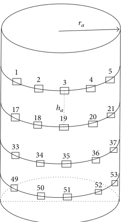
Here we derive the model for the receiver array used in the measurement using the above phase-shift model. Figure5
shows a cylindrical antenna array with 4 rings of 16-element array mounted on the cylindrical surface. The radiance of the cylinder is𝑟𝑎and the distance between the rings isℎ𝑎.
We can identify the distance differences by the geometric relationship. The distance difference has four possible values
as in (11) and (12) for the two inner rings of elements and as in (13) and (14) for the two outer rings of elements, where𝑑0is the distance between the transmitter and the array centre in the horizontal plane;𝜙𝑖is the azimuth angle of the𝑖th element with respect to the reference direction. Consider
Δ𝑑1= (𝑟𝑎2+ 𝑑2+14ℎ2𝑎− ℎ𝑎√𝑑2− (𝑑0+ 𝑟𝑎)2
−2𝑟 (𝑑0+ 𝑟𝑎)cos𝜙𝑖)
1/2 ,
(11)
Δ𝑑2= (𝑟𝑎2+ 𝑑2+1
4ℎ2𝑎+ ℎ𝑎√𝑑2− (𝑑0+ 𝑟𝑎)2
−2𝑟 (𝑑0+ 𝑟𝑎)cos𝜙𝑖)1/2,
(12)
Δ𝑑3= (𝑟2
𝑎+ 𝑑2+94ℎ2𝑎− 3ℎ𝑎√𝑑2− (𝑑0+ 𝑟𝑎)2
−2𝑟 (𝑑0+ 𝑟𝑎)cos𝜙𝑖)
1/2 ,
(13)
Δ𝑑4= (𝑟𝑎2+ 𝑑2+94ℎ2𝑎+ 3ℎ𝑎√𝑑2− (𝑑0+ 𝑟𝑎)2
−2𝑟 (𝑑0+ 𝑟𝑎)cos𝜙𝑖)
1/2 ,
(14)
R(𝜔)
= [𝑒−2𝑗𝜋Δ𝑑3/𝜆 ⋅ ⋅ ⋅ 𝑒−2𝑗𝜋Δ𝑑1/𝜆 ⋅ ⋅ ⋅ 𝑒−2𝑗𝜋Δ𝑑2/𝜆 ⋅ ⋅ ⋅ 𝑒−2𝑗𝜋Δ𝑑4/𝜆 ⋅ ⋅ ⋅] .
(15)
Thus, the array response vector is written as (15). In this equation the array response can be uniformly divided into 4 parts corresponding to the 4 rings of elements. Each part contains a 16-element vector corresponding to the 16 elements in each ring. With the ray-launching model to feed the rays as the input, we can obtain the complete channel matrix.
A similar phase-shift model has also been used in MIMO channel modelling in [16]. However, using only a single ray to approximate the whole array has low accuracy, especially for modelling large array systems. Therefore, we can further choose more representative rays to model the large size array to improve accuracy. For example, in the cylindrical array in Figure5, we can model the cylindrical array as 4 layers of 2D uniform circular array. Each consists of 16 antenna elements. Thus, instead of choosing the cylindrical array centre as the reference point, we choose the centres of the 4 layers of the 2D circular array. We then have 4 rays to approximate the whole channel matrix.
In this case, the distance difference is given as
Δ𝑑𝑖(𝑝) = √𝑟2
𝑎+ 𝑑2(𝑝) − 2𝑟(𝑑0+ 𝑟𝑎)cos𝜙𝑖− 𝑑𝑖(𝑝) ,
for 𝑝 = {1, 2, 3, 4} ,
(16)
[image:4.600.323.551.136.410.2]R(𝜔) = [𝑒−2𝑗𝜋Δ𝑑1(1)/𝜆 ⋅ ⋅ ⋅ 𝑒−2𝑗𝜋Δ𝑑17(2)/𝜆 ⋅ ⋅ ⋅ 𝑒−2𝑗𝜋Δ𝑑33(3)/𝜆 ⋅ ⋅ ⋅ 𝑒−2𝑗𝜋Δ𝑑49(4)/𝜆 ⋅ ⋅ ⋅] . (17)
This model requires the ray-launching simulation of4rays. It compensates the accuracy by higher computational cost than the single ray model. We name this model as the simplified deterministic model in the following part of this paper.
2.3. Ray-Launching Based Statistical Model. Modelling the wireless channel as a probabilistic fading channel is another category of channel models in contrast to the deterministic channel models. It has the advantage of simplicity and effi-ciency when physical model is prohibitively complex. In this part, we propose a probabilistic channel model for massive MIMO based on the ray-launching model. Considering that the model is specifically for indoor scenario, we model the fading channel as Rician distribution. The choice of Rician distribution is because it comprises a rich group of probability distributions: by determining various values for the Rician𝐾 factor, a group of statistical distributions is included. The ray-launching model supplies the multipath information to esti-mate the parameters for the Rician distribution. Furthermore, the channel measurement also indicates that the channel elements follow a Rician distribution. A recent study to model the massive MIMO as a Rician distributed statistical model can be found in [17].
A single antenna Rician distributed channel can be written as
ℎ = √𝑘ℎ𝑑+ √1 − 𝑘ℎ𝑠, (18)
where𝑘is the𝐾factor in Rician distribution,ℎ𝑑is the direct path component, andℎ𝑠is the scattering component.
We model the channel matrix element𝐻𝑚,𝑛 in (1) as a Rician distributed random variable:
𝐻𝑚,𝑛∼Rice(V, 𝜎) , (19)
whereVand 𝜎 are the parameters to determine the Rician distribution. The probability distribution function of the Rician distribution is given as
𝑓 (𝑥 |V, 𝜎) = 𝜎𝑥2(− (𝑥
2+ 𝜎2)
2𝜎2 ) 𝐼0(
𝑥V
𝜎2) , (20)
where𝐼0(⋅)is the modified Bessel function of the first kind with order zero. In order to obtain the exact distribution function, we need to estimate the two parametersVand𝜎. We will resort to the ray-launching model to estimate these two parameters.
The ray-launching model traces a group of rays equivalent to the multipath components. This multipath information can be used to estimate the parameters of the Rician distribution. Below we adopt the method from the work of [18] to estimate the Rician distribution parameters.
The rays are modelled as equivalent to the multipath components in (3). From this model, we have the values of the ray field𝐴𝛼 along each ray. We can use this multipath information to estimate the parametersV and 𝜎 as shown below.
According to [18] the𝑘-factor can be estimated as
𝑘 = √1 − 𝑟
1 − √1 − 𝑟. (21)
The quantity𝑟is given as
𝑟 = 𝑉 [𝐴
2]
(𝐸 [𝐴2])2, (22)
where𝑉[𝐴2]is the variance of𝐴2.
After obtaining the 𝑘-factor, the Rician distribution parametersVand𝜎can be calculated from
V2= 1 + 𝑘𝑘 Ω,
𝜎2= 1
2 (1 + 𝑘)Ω,
(23)
whereΩ = 𝐸[𝐴2]is the expected value of the𝐴2. Thus, we obtain the two parametersVand𝜎.
Then we can write the MIMO channel matrix as
H=
[ [ [ [ [ [ [ [ [ [
𝐻1,1∼Rice(V1,1, 𝜎1,12 ) 𝐻1,1∼Rice(V1,2, 𝜎1,22 ) ⋅ ⋅ ⋅ 𝐻1,𝑟∼Rice(V1,𝑟, 𝜎1,𝑟2 )
𝐻2,1∼Rice(V2,1, 𝜎2,12 ) 𝐻2,2∼Rice(V2,2, 𝜎2,22 ) ⋅ ⋅ ⋅ 𝐻2,𝑟∼Rice(V2,𝑟, 𝜎2,𝑟2 )
..
. ... d ...
𝐻𝑡,1∼Rice(V𝑡,1, 𝜎2𝑡,1) 𝐻𝑡,2∼Rice(V𝑡,1, 𝜎2𝑡,1) ⋅ ⋅ ⋅ 𝐻𝑡,𝑟∼Rice(V𝑡,𝑟, 𝜎2𝑡,𝑟)
] ] ] ] ] ] ] ] ] ]
where V𝑡,𝑟 is the V parameter estimated between the 𝑟th
receiver and the𝑡th transmitter. We name this model as the statistical model in the following part of the paper.
This probabilistic MIMO model requires the calculation ofVand𝜎parameters for each channel matrix element. Such a statistical model still requires the input from the determinis-tic ray-launching model. But it has the advantage of flexibility in real application since the only parameters required are the parameters for the probability distributions. Moreover, the calculation repeats the ray-launching simulation until all the matrix elements are computed. Such a process costs high computational resource in simulation. We can further simplify the calculation process in the following part.
2.4. Simplified Statistical Model Using Phase-Shift. Similar to the simplified deterministic model for massive MIMO chan-nel, we can choose one representative point to approximate the whole antenna array. Although such an approximation sacrifices certain accuracy, it significantly reduces the com-putational cost by decreasing the repetition of ray-launching model simulation to only once.
Here again we choose the array center as the representa-tive point to calculate the probability distribution parameters
V and 𝜎 for the whole channel matrix. Thus, the channel matrix is written as
H=
[ [ [ [ [ [
𝐻1,1∼Rice(V𝑐, 𝜎𝑐2) 𝐻1,1∼Rice(V𝑐, 𝜎𝑐2) ⋅ ⋅ ⋅ 𝐻1,𝑟∼Rice(V𝑐, 𝜎𝑐2)
𝐻2,1∼Rice(V𝑐, 𝜎𝑐2) 𝐻2,2∼Rice(V𝑐, 𝜎𝑐2) ⋅ ⋅ ⋅ 𝐻2,𝑟∼Rice(V𝑐, 𝜎𝑐2)
..
. ... d ...
𝐻𝑡,1∼Rice(V𝑐, 𝜎2𝑐) 𝐻𝑡,2∼Rice(V𝑐, 𝜎𝑐2) ⋅ ⋅ ⋅ 𝐻𝑡,𝑟∼Rice(V𝑐, 𝜎2𝑐)
] ] ] ] ] ]
, (25)
where V𝑐 and 𝜎𝑐 are parameters estimated using the rays
between the transmitters and the center of the receiver array. Like the simplified deterministic model, this model shows adequate accuracy in many applications. We name this model the simplified statistical model. We will show the comparison result between this model and the measurement in Section4.1.
3. Measurement Campaigns
Small cell and heterogeneous wireless networks, such as femtocell and wireless local area network (WLAN), are the major networks to be deployed for the next generation of wireless networks. These small networks are mainly deployed in indoor environments as a complement to the larger cell networks, to deploy heterogeneous networks. The measure-ments are carried out in indoor environmeasure-ments. They are typical small cell wireless network deployment scenarios. Equipped with massive MIMO antenna arrays, they are interesting scenarios for studying the performance of next generation wireless networks with massive MIMO channels. We have carried out two measurement campaigns for the indoor cellular networks: downlink and uplink scenarios. We give the details of the channel measurements in the following part of this section. As our primary concern is network planning for indoor networks, the measurement in the uplink scenario was carried out with the receiver at a fixed location. In the downlink scenario, the transmitter stayed in a fixed location.
For channel modelling, such 2 scenarios have little differ-ence on the channel modelling. However, for measurement, we intended to measure the channel with accuracy in real network applications. Furthermore, due to the limitation of mobility of the equipment, the measurements in these 2 environments fall into the network application scenarios
of downlink and uplink. Moreover, the two environments have different characteristics. The uplink scenario contains complex walls and windows structure. The downlink scenario is relatively simple environment. The two different scenarios also showed the flexibility and adaptability of the IRLA model.
3.1. Measurement of Downlink Channel. The downlink chan-nel is measured in an indoor office environment. The mea-surement site is in the Electrical Engineering Department at Lund University, Sweden. Figure6 shows a map of the building floor.
The antenna array equipped at the transmitter is a flat panel antenna array with 64 dual-polarised patch antenna elements. Figure8(a)shows a photo of the transmitter array. The receiver array is a cylindrical array with 64 dual-polarised patch antenna elements. Figure8(b)shows a photo of the receiver array. These antenna arrays are both with 64 antenna elements. They are typical massive MIMO antenna arrays. We choose to use these antenna arrays to carry out the measurement campaign to study the performance of massive MIMO channel. The frequency of the channel measurement is 2.6 GHz. The transmitter power is set to be 20 dBm to 40 dBm depending on the locations.
The measurement has been carried out in the rooms shown in Figure6. The transmitter is fixed at the location𝑇𝑥. The receivers are moved from location 1 to location 9. This is a typical downlink scenario in indoor small cell networks. We measure the channel matrices at the 9 locations marked in the map.
23
25
23
24
23
23
23
22
23
21
23
20
A
23
20
B
23
13
23
14 2315
23
19
23
20
C
23
12
6 5 4
8 9
3 2 1
TX
23
16
/
23
17
/
23
18
23
26
/
23
27
[image:7.600.104.497.77.250.2]7
Figure 6: Building floor map of the downlink scenario.
have also been used to measure MIMO channel with small number of antennas in the work of [19]. Figure7shows a map of the building floor.
The transmitter antenna array is a 32-element antenna array with 4 layers of 8-element uniform linear arrays. Each antenna element has an omnidirectional radiation pattern. The receiver antenna array has a similar structure with 4 layers of 6-element uniform linear arrays.
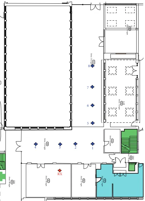
The measurement scenario is shown as the building map in Figure 7. The receiver is fixed at the location 𝑅𝑥. The transmitter is moved from location 1 to location 8. The frequency of of the channel measurement is 2.4 GHz. This is a typical uplink scenario in the indoor small cell networks. We measure the channel matrix at the 8 locations marked in the map.
4. Measurement and Simulation Comparison
and Analysis
The prediction of the channel is based on the simulation of the IRLA. It has shown to achieve accuracy close to FDTD like models in indoor environment [13]. Additionally, it is optimised for achieving high computational efficiency, especially for the purpose of network planning. Further details of the IRLA have been presented in the work of [13]. We use the IRLA to predict the MIMO channels in this section.
For outdoor MIMO channel modelling, the work of [20–
22] focused on the MIMO modelling based on ray-tracing simulation. These works showed that diffuse scattering is a key factor in the outdoor MIMO modelling. For complex outdoor environment, diffusive scattering has an impact on the angular spread of the propagation channel and further determines the performance of the MIMO channel. However, for the indoor channel, the key is to model the environment with details. The work of [23] gave an example of MIMO channel modelling in indoor environment. The authors
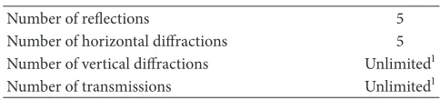
Table 1: Simulation settings.
Number of reflections 5
Number of horizontal diffractions 5
Number of vertical diffractions Unlimited1
Number of transmissions Unlimited1
1Until signal strength is under threshold.
modelled the details of the complex indoor structure using FDTD method. Combining with a ray-tracing method, a satisfying result was achieved. The IRLA model has shown to achieve accuracy close to FDTD like models in [13] by modelling the details of the environment into the simulation. The model further incorporated a parameter calibration process to determine the optimal values of the parameters to minimise the prediction errors.
The IRLA simulation requires the detailed information of the environment. The environmental information includes the structures and materials of the environments. The struc-ture of the building is imported through the construction map of the buildings. The walls, doors, and windows struc-tures are all included in the simulation model. The construc-tion material informaconstruc-tion is provided. It is matched with a material database supported by the IRLA. Figure9gives the 3D view of the modelled environment in the downlink scenario. The figure shows that the windows, doors, walls, and tables are modelled in the simulation. Additionally, the simulation model settings are given in Table1. It gives the number of interactions in the IRLA simulation.
[image:7.600.307.549.330.385.2]1 2 3 4
5 6 7 8
RX
222
224
202 2202
289
287 286 285
2201
220
201
219
Ar
ea
:
114
sq
m
LA
B
Ar
ea
:
72
sq
m
Ar
ea
:
51
sq
m
Ar
ea
:
13
2
sq
m
Ar
ea
:
13
sq
m
Ar
ea
:
30
sq
m
Ar
ea
:
17
sq
m
Ar
ea
:
27
sq
m
Ar
ea
:
50
sq
m
Ar
ea
:
48
sq
[image:8.600.183.418.82.408.2]m
Figure 7: Building floor map of the uplink scenario.
(a) (b)
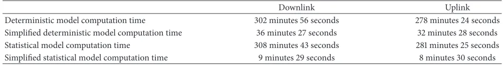
[image:8.600.124.476.460.705.2]Table 2: Computation time of the models.
Downlink Uplink
Deterministic model computation time 302 minutes 56 seconds 278 minutes 24 seconds Simplified deterministic model computation time 36 minutes 27 seconds 32 minutes 28 seconds Statistical model computation time 308 minutes 43 seconds 281 minutes 25 seconds Simplified statistical model computation time 9 minutes 29 seconds 8 minutes 30 seconds
[image:9.600.84.257.175.276.2]7
Figure 9: 3D view of the simulation environment of the downlink scenario.
were written in a vector form. The root mean square (RMS) error between the prediction using the parameters(𝜇𝑖, 𝜖𝑗)and the measurement was given as
RMSE𝑖,𝑗= 1
𝑟𝑡 𝑚=𝑟,𝑛=𝑡
∑
𝑚=1,𝑛=1√𝐻
2
𝑚,𝑛− ̂𝐻(𝑖, 𝑗)2𝑚,𝑛, (26)
where 𝐻(𝑖, 𝑗)̂ 𝑚,𝑛 is the simulated channel matrix using the parameters (𝜇𝑖, 𝜖𝑗). The calibration aims to minimise this RMS error by tuning the propagation parameters:
(𝜇, 𝜖) =arg min𝜇
𝑖,𝜖𝑗(RMSE𝑖,𝑗)
2
. (27)
The calibration process is executed in an iterative way between the parameter estimation and the ray-launching simulation. This calibration process was implemented using the simulated annealing algorithm. In practice the algorithm usually converges to achieve the minimum error.
4.1. Computational Efficiency. In this section, we first present the computation time of the 4 models, using them to simulate the downlink and uplink scenarios. Table2shows the computation time the 4 models take to simulate the downlink scenario and uplink scenario. We adopt the same simulation setting as in the work of [12]. The simulation resolution is set to be 0.1 m. We can see that for a massive MIMO system the calculation of MIMO matrices for a typical indoor environment can take several hours. In our simulation Model 1 and Model 3 take about 5 hours to simulate the whole environment. The results also show that Model 2 and Model 4 use a significant less amount of time than Model 1 and Model 3. This is due to the lower computational complexity of both Model 2 and Model 4. Model 1 and Model 3 both calculate each individual channel matrix element via ray-launching, while Model 2 and Model 4 reduce the times of repetition for ray-launching simulation.
The computational cost in the simulation is mainly due to the ray-launching simulation. The computation time is linear in the repetition of the ray-launching simulation. For Model 4 the ray-launching algorithm only simulates once; Model 2 simulates 4 times; Model 1 and Model 3 both simulate 32 times. The computation time listed in Table2agrees with this analysis.
This result suggests that, for time demanding tasks in network planning and optimisation applications, both the simplified models, Model 2 and Model 4, are better choices.
4.2. Received Signal Power. The received signal power is one of the most important parameters in network deployment and optimisation. It is closely related to the performance of the wireless networks. According to (3) the received power at a certain location is calculated as
𝑃 (𝑥, 𝑦, 𝑧) =
𝑞 ∑ 𝛼=1
𝐴𝛼(𝑥, 𝑦, 𝑧) 𝑒−𝑗𝜔0𝜏𝛼(𝑥,𝑦,𝑧)
2
. (28)
Figure 10 shows the comparison between the average received power of the measurements and the simulation results in the downlink scenario. Figure11shows the same comparison result in the uplink scenario. We can see that both results show good agreements.
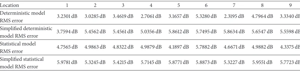
According to (26), we use the simulated channel𝐻̂𝑚,𝑛and the measured channel𝐻𝑚,𝑛to calculate the RMS errors of the simulation models. The RMS error results are presented in Tables3and4.
The results show that the RMS errors of Model 1 and Model 3 are smaller. The RMS errors of Model 2 and Model 4 are higher but still mostly under 6 dB. This shows that the accuracy of Model 1 and Model 3 is higher than that of Model 2 and Model 4. This is because both Model 2 and Model 4 simplify the computation by using a single ray to represent the whole array. The two simplified models trade certain degree of accuracy for computational efficiency. However, the result shows that the overall accuracy of the ray-launching models for massive MIMO systems is satisfying for the network planning and optimisation purpose.
Table 3: Received signal power RMS error in downlink scenario.
Location 1 2 3 4 5 6 7 8 9
Deterministic model 3.2301 dB 3.0285 dB 3.4619 dB 2.7061 dB 3.1657 dB 5.3280 dB 2.3195 dB 4.7964 dB 3.3340 dB RMS error
Simplified deterministic 3.7594 dB 5.4562 dB 5.4561 dB 5.0356 dB 5.8612 dB 5.7495 dB 5.8634 dB 5.6547 dB 5.5598 dB model RMS error
Statistical model
4.7565 dB 4.9863 dB 4.8322 dB 4.9879 dB 4.1897 dB 5.7882 dB 4.6671 dB 4.9882 dB 4.3375 dB RMS error
Simplified statistical
[image:10.600.49.549.255.370.2]5.9781 dB 5.3245 dB 5.4215 dB 5.7145 dB 5.8771 dB 5.8873 dB 5.3227 dB 5.9551 dB 5.7723 dB model RMS error
Table 4: Received signal power RMS error in uplink scenario.
Location 1 2 3 4 5 6 7 8
Deterministic model 2.9568 dB 2.2584 dB 3.6514 dB 3.9184 dB 2.3808 dB 2.3101 dB 2.8085 dB 2.2751 dB RMS error
Simplified deterministic 5.8631 dB 5.7761 dB 4.3343 dB 5.4475 dB 5.2403 dB 5.9712 dB 5.3315 dB 5.9882 dB model RMS error
Statistical model
4.7701 dB 4.2321 dB 4.5642 dB 5.4241 dB 4.0214 dB 4.0859 dB 4.8794 dB 4.9583 dB RMS error
Simplified statistical
5.4578 dB 5.3762 dB 5.4772 dB 5.6549 dB 5.6873 dB 5.0857 dB 5.7544 dB 5.7563 dB model RMS error
Simplified statistical model
1 2 3 4 5 6 7 8 9
−120 −110 −100 −90 −80 −70 −60 −50 −40 −30
Measurement locations
Recei
ve
d p
ow
er (dB
m)
[image:10.600.314.544.408.655.2]Measurement Deterministic model Simplified deterministic model Statistical model
Figure 10: Average received power in downlink.
In Figure 12 we present the cumulative distribution function (CDF) of the simulated channel matrix elements of the downlink scenario in comparison with the measurement.
1 2 3 4 5 6 7 8
−90 −80 −70 −60 −50 −40 −30 −20
Measurement locations
Recei
ve
d p
ow
er (dB
m)
Measurement Deterministic model Simplified deterministic model Statistical model
[image:10.600.56.289.411.652.2]Simplified statistical model
Figure 11: Average received power in uplink.
−65 −64 −63 −62 −61 −60 −59 −58 −57 −56 0
0.1 0.2 0.3 0.4 0.5 0.6 0.7 0.8 0.9 1
x
Empirical (CDF)
Measurement Deterministic model Statistical model
Simplified Statistical model
F(
[image:11.600.315.542.68.317.2]X)
Figure 12: Distribution of received power of channel elements in downlink.
0 0.1 0.2 0.3 0.4 0.5 0.6 0.7 0.8 0.9
1 Empirical (CDF)
Measurement Deterministic model Statistical model
Simplified Statistical model
−64 −63 −62 −61 −60 −59 −58 −57
F(
X)
X
Figure 13: Distribution of received power of channel elements in uplink.
have a very close distribution to the measured channel matrix elements. This demonstrates a good agreement between the simulation model and the measurement.
The uplink scenario result in Figure13shows a similar pattern as in the downlink scenario. The above results demonstrate that the simulation models generate channel matrix elements with good agreements to the measurement.
1 2 3 4 5 6 7 8 9
15 20 25 30
35 40 45
Measurement locations
Cha
n
nel ca
paci
ty (b
its/s/H
z)
Measurement Deterministic model
Simplified Deterministic model Statistical model
[image:11.600.56.286.72.314.2]Simplified Statistical model
Figure 14: Channel capacity in downlink.
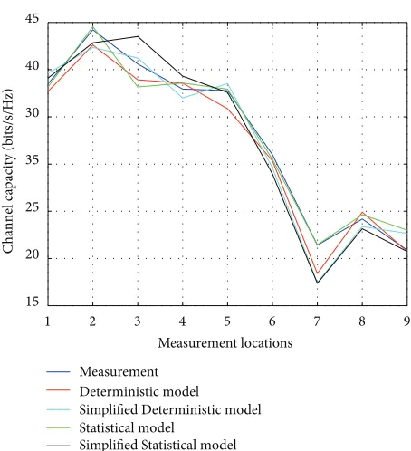
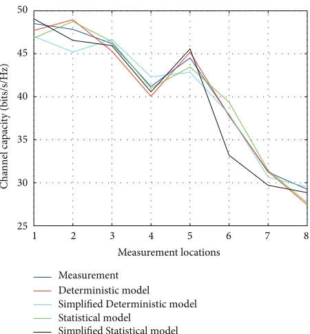
4.4. Channel Capacity Results. Channel capacity gain is one of the most attractive features of the massive MIMO channel promised to the future wireless networks. In this part of the result, we present the channel capacity comparison between the simulated channels and the measurement.
The MIMO channel capacity is calculated according to the equation given in [24,25] as
𝐶 =E(log det(I+ 𝑃𝑡
𝑛𝑁0HH∗)) , (29)
whereE(⋅)represents the expectation,𝑃𝑡is the total transmit power, and𝑛is the number of transmitter antennas.
We apply the above MIMO channel capacity formula to calculate the MIMO channel capacity from both the simu-lated channel matrices and the measured channel matrices. Figure14shows the capacity result comparison in the down-link scenario. Figure15shows the capacity result comparison in the uplink scenario. Both figures show a good agreement in the channel capacity between the simulated results and the measurement. This demonstrates that the simulation models are accurate in estimating the channel capacity. Therefore, the simulation models provide a reliable way to predict the channel capacity in network planning and optimisation.
5. Conclusion
[image:11.600.56.287.359.607.2]50
45
40
35
30
25
1 2 3 4 5 6 7 8
Measurement locations
Cha
n
nel ca
paci
ty (b
its/s/H
z)
Measurement Deterministic model
Simplified Deterministic model Statistical model
[image:12.600.59.284.71.314.2]Simplified Statistical model
Figure 15: Channel capacity in uplink.
deployment environments. The comparison results show that the models have good agreements with the measurement. This demonstrates that these ray-launching based simulation models are efficient and accurate models, for planning and optimising indoor networks equipped with massive MIMO arrays.
Conflict of Interests
The authors declare that they have no conflict of interests regarding to the publication of this paper.
Acknowledgments
The first author would like to thank Mr. Cheng Fang, Dr. Andres Alayon Glasunov, and Professor Fredrik Tufvesson for the measurement campaign carried out in Lund Univer-sity and Mr. Nasoruddin Mohamad and Mr. Adnan Cheema for the measurement campaign carried out in Durham University. The work was supported by the EU FP7 Project WiNDOW.
References
[1] F. Boccardi, R. W. Heath Jr., A. Lozano, T. L. Marzetta, and P. Popovski, “Five disruptive technology directions for 5G,”IEEE Communications Magazine, vol. 52, no. 2, pp. 74–80, 2014. [2] F. Rusek, D. Persson, B. K. Lau et al., “Scaling up mimo:
opportunities and challenges with very large arrays,” IEEE Signal Processing Magazine, vol. 30, no. 1, pp. 40–60, 2013. [3] E. G. Larsson, F. Tufvesson, O. Edfors, and T. L. Marzetta,
“Massive MIMO for next generation wireless systems,”IEEE Communications Magazine, vol. 52, no. 2, pp. 186–195, 2014.
[4] Z. Lai, N. Bessis, G. de la Roche, P. Kuonen, J. Zhang, and G. Clapworthy, “On the use of an intelligent ray launching for indoor scenarios,” inProceedings of the 4th European Conference on Antennas and Propagation (EuCAP ’10), pp. 1–5, April 2010. [5] A. Burr, “Evaluation of capacity of indoor wireless mimo
chan-nel using ray tracing,” inProceedings of the International Zurich Seminar on Broadband Communications: Access, Transmission, Networking, pp. 28-1–28-6, 2002.
[6] S.-. Oh and N.-. Myung, “MIMO channel estimation method using ray-tracing propagation model,”Electronics Letters, vol. 40, no. 21, pp. 1350–1352, 2004.
[7] Y. Gao, X. Chen, and C. Parini, “Experimental evaluation of indoor mimo channel capacity based on ray tracing,” in
Proceedings of the London Communications Symposium, pp. 189–192, University College London, 2004.
[8] O. St¨abler, “Mimo channel characteristics computed with 3d ray tracing model,” inProceedings of the COST2100 TD(08) Workshop, Trondheim, Norway, June 2008.
[9] S. Loredo, A. Rodr´ıguez-Alonso, and R. P. Torres, “Indoor MIMO channel modeling by rigorous GO/UTD-based ray tracing,”IEEE Transactions on Vehicular Technology, vol. 57, no. 2, pp. 680–692, 2008.
[10] R. Hoppe, J. Ramuh, H. Buddendick, O. St¨abler, and G. W¨olfle, “Comparison of MIMO channel characteristics computed by 3D ray tracing and statistical models,” inProceedings of the 2nd European Conference on Antennas and Propagation (EuCAP ’07), pp. 1–5, November 2007.
[11] J. Gorce, K. Jaffr`es-Runser, and G. de la Roche, “Deterministic approach for fast simulations of indoor radio wave propaga-tion,”IEEE Transactions on Antennas and Propagation, vol. 55, no. 3, pp. 938–948, 2007.
[12] X. Tu, H. Hu, Z. Lai, J.-M. Gorce, and J. Zhang, “Performance comparison of MR-FDPF and ray launching in an indoor office scenario,” in Proceedings of the Loughborough Antennas and Propagation Conference (LAPC '13), pp. 424–428, Loughbor-ough, UK, November 2013.
[13] Z. Lai, G. De La Roche, N. BESSIS et al., “Intelligent ray launching algorithm for indoor scenarios,”Radioengineering, vol. 20, no. 2, pp. 398–408, 2011.
[14] B. Clerckx and C. Oestges,MIMO Wireless Networks: Channels, Techniques and Standards for Multi-Antenna, Multi-User and Multi-Cell Systems, Academic Press, 2nd edition, 2013. [15] G. German, Q. Spencer, L. Swindlehurst, and R. Valenzuela,
“Wireless indoor channel modeling: Statistical agreement of ray tracing simulations and channel sounding measurements,” in Proceedings of IEEE Interntional Conference on Acoustics, Speech, and Signal Processing (ICASSP ’01), vol. 4, pp. 2501–2504, May 2001.
[16] J. Voigt, R. Fritzsche, and J. Schueler, “Optimal antenna type selection in a real SU-MIMO network planning scenario,” in
Proceedings of the 70th IEEE Vehicular Technology Conference (VTC ’09), pp. 1–5, September 2009.
[17] S. Payami and F. Tufvesson, “Channel measurements and analysis for very large array systems at 2.6 GHz,” inProceedings of the 6th European Conference on Antennas and Propagation (EuCAP ’12), pp. 433–437, March 2012.
[18] A. Abdi, C. Tepedelenlioglu, M. Kaveh, and G. Giannakis, “On the estimation of the K parameter for the rice fading distribution,”IEEE Communications Letters, vol. 5, no. 3, pp. 92– 94, 2001.
ghz frequency band,”Radio Science, vol. 44, no. 5, Article ID 10.1029/2008RS004095, pp. 10–1029, 2009.
[20] A. Richter, J. Salmi, and V. Koivunen, “Distributed scattering in radio channels and its contribution to MIMO channel capacity,” inProceedings of the European Conference on Antennas and Propagation (EuCAP ’06), pp. 1–7, Nice, France, November 2006.
[21] F. Mani, F. Quitin, and C. Oestges, “Directional spreads of dense multipath components in indoor environments: experimental validation of a Ray-Tracing approach,”IEEE Transactions on Antennas and Propagation, vol. 60, no. 7, pp. 3389–3396, 2012. [22] E. Vitucci, V. Degli-Esposti, and F. Fuschini, “Mimo channel
characterization through ray tracing simulation,” inProceedings of the 1st European Conference on Antennas and Propagation (EuCAP ’06), pp. 1–6, November 2006.
[23] Z. Yun, M. Iskander, and Z. Zhang, “Mimo capacity calculation and fading estimation for indoor/outdoor wireless commu-nication environments,” in Proceedings of the IEEE Topical Conference on Wireless Communication Technology, pp. 259– 260, October 2003.
[24] E. Telatar, “Capacity of multi-antenna Gaussian channels,”
European Transactions on Telecommunications, vol. 10, no. 6, pp. 585–595, 1999.
[25] G. J. Foschini and M. J. Gans, “On limits of wireless communi-cations in a fading environment when using multiple antennas,”
International Journal of
Aerospace
Engineering
Hindawi Publishing Corporation
http://www.hindawi.com Volume 2014
Robotics
Journal ofHindawi Publishing Corporation
http://www.hindawi.com Volume 2014
Hindawi Publishing Corporation
http://www.hindawi.com Volume 2014
Active and Passive Electronic Components
Control Science and Engineering
Journal of
Hindawi Publishing Corporation
http://www.hindawi.com Volume 2014
Machinery
Hindawi Publishing Corporation
http://www.hindawi.com Volume 2014 Hindawi Publishing Corporation
http://www.hindawi.com
Journal of
Engineering
Volume 2014
Submit your manuscripts at
http://www.hindawi.com
VLSI Design
Hindawi Publishing Corporation
http://www.hindawi.com Volume 2014
Hindawi Publishing Corporation
http://www.hindawi.com Volume 2014 Shock and Vibration
Hindawi Publishing Corporation
http://www.hindawi.com Volume 2014
Civil Engineering
Advances inAcoustics and VibrationAdvances in
Hindawi Publishing Corporation
http://www.hindawi.com Volume 2014
Hindawi Publishing Corporation
http://www.hindawi.com Volume 2014 Electrical and Computer Engineering
Journal of
Advances in OptoElectronics
Hindawi Publishing Corporation
http://www.hindawi.com Volume 2014
The Scientific
World Journal
Hindawi Publishing Corporationhttp://www.hindawi.com Volume 2014
Sensors
Journal ofHindawi Publishing Corporation
http://www.hindawi.com Volume 2014
Modelling & Simulation in Engineering Hindawi Publishing Corporation
http://www.hindawi.com Volume 2014
Hindawi Publishing Corporation
http://www.hindawi.com Volume 2014 Chemical Engineering
International Journal of Antennas and Propagation International Journal of
Hindawi Publishing Corporation
http://www.hindawi.com Volume 2014
Hindawi Publishing Corporation
http://www.hindawi.com Volume 2014 Navigation and Observation International Journal of
Hindawi Publishing Corporation
http://www.hindawi.com Volume 2014