Probabilistic uncertainty analysis of an FRF of a structure using a Gaussian process emulator

promoting access to White Rose research papers

White Rose Research Online

[email protected]

Universities of Leeds, Sheffield and York

http://eprints.whiterose.ac.uk/

This is an author produced version of a paper due to be published in

Mechanical

Systems and Signal Processing

.

White Rose Research Online URL for this paper:

Published paper

Fricker, T.E., Oakley, J.E., Sims, N.D., Worden, K. (2011)

Probabilistic

uncertainty analysis of an FRF of a structure using a Gaussian process emulator

,

Mechanical Systems and Signal Processing (In Press)

Probabilistic uncertainty analysis of an FRF of a

structure using a Gaussian process emulator

Thomas E. Frickera, Jeremy E. Oakleyb, Neil D. Simsc, Keith Wordend

a

Corresponding author.

Department of Probability and Statistics, University of Sheffield, Sheffield S3 7RH, UK

Tel: +44 (0)114 222 3801. Fax: +44 (0)114 222 3809. Email: [email protected].

b

Department of Probability and Statistics, University of Sheffield, Sheffield S3 7RH, UK.

Email: [email protected]

c

Department of Mechanical Engineering, University of Sheffield, Sheffield S1 3JD, UK.

Email: [email protected]

d

Department of Mechanical Engineering, University of Sheffield, Sheffield S1 3JD, UK.

Email:[email protected]

Abstract

This paper introduces methods for probabilistic uncertainty analysis of a fre-quency response function (FRF) of a structure obtained via a finite element (FE) model. The methods are applicable to computationally expensive FE

models, making use of a Bayesian metamodel known as anemulator. The

em-ulator produces fast predictions of the FE model output, but also accounts for the additional uncertainty induced by only having a limited number of model evaluations. Two approaches to the probabilistic uncertainty analysis of FRFs are developed. The first considers the uncertainty in the response at discrete frequencies, giving pointwise uncertainty intervals. The second considers the uncertainty in an entire FRF across a frequency range, giving an uncertainty envelope function. The methods are demonstrated and compared to alternative approaches in a practical case study.

Keywords: finite element model, probabilistic uncertainty analysis, envelope frequency response function, Gaussian process, metamodel, Bayesian

1. Introduction

(for example due to assumptions regarding the boundary conditions), or alter-natively they could arise due to unknown values of physical parameters (for example component geometry or material properties). In the latter case, this lack of knowledge could be attributed to variation between nominally identical components (i.e. variability), or uncertainty during the design process regarding the final choice of dimensions or material.

There has long been interest in how uncertainty propagates through FE models. The method with the greatest pedigree is the Stochastic Finite El-ement method (SFE) [1]; this is a probabilistic method. In the general SFE formulation, the material properties across the structure can be specified as a random field. In a manner similar to the discretisation of the structure into finite elements, the random field is discretised into a denumerable set of ran-dom variables using the Karhunen-Loeve expansion, which is then truncated at some finite order. The results from the FE model are then expressed as a mean value supplemented by an expansion in terms of the random variables, allowing statistics of the quantity of interest to be computed. In the last decade, interest has grown in possibilistic approaches, such as a fuzzy approach to FE analysis and computation of modal quantities [2, 3]. More recent work has considered component mode synthesis as a framework for investigating both probabilistic and possibilistic uncertainties [4], and using possibilistic techniques based upon fuzzy numbers [5]. A ‘fuzzy FE’ approach is also developed in [6] and applied to a variety of case studies including the Garteur benchmark FE problem - a small scale aircraft model developed for assessing ground vibration test techniques.

A common issue when trying to propagate uncertain parameters through complex FE models is that the deterministic nature of the modelling approach leads to many model evaluations being performed, each for a different configu-ration of the uncertain inputs. In probabilistic modelling, this results in Monte Carlo simulations, whilst in possibilistic modelling, the repeated model evalua-tions can be used to generate fuzzy numbers representing the uncertainty in the model’s response.

This paper focusses on a probabilistic method for uncertainty analysis of FE models, using a statistical metamodel, or emulator, to reduce the number of FE model evaluations required, and hence reduce the computational cost. The remainder of the paper is organised as follows. First, the probabilistic uncertainty analysis problem is formulated, before introducing the concept of the emulator. Next, the use of the emulator for uncertainty analysis is described using a simple graphical example. The uncertainty analysis of FRFs that are predicted from FE models is then considered. This approach is then applied to a numerical case study based upon the Garteur testbed. Following a discussion, conclusions are drawn regarding the application of this modelling approach to FE modelling problems in structural dynamics.

2. Probabilistic uncertainty analysis of FE models

Consider a deterministic FE model evaluated at a particular degree of

returns a set of outputs that consists of pairs of modal parameters. A typi-cal FE analysis considers a subset of the modal parameters, which we denote

{( ˆmi,ˆki) :i= 1, ...nmodes}, where ˆmiare the modal masses and ˆkiare the modal stiffnesses. The FE model is deterministic, so repeated runs with the same con-figuration of input parameters will return the same outputs, and we may

repre-sent it as a functiony=η(x), wherey= ( ˆm1,ˆk1,mˆ2,kˆ2, ...,mˆnmodes,kˆnmodes)

T_.

In the probabilistic uncertainty analysis of a deterministic computer model, we consider the values of the uncertain input parameters to be a multivariate

random variableX. As a result, the output of the model is also a multivariate

random variable, which we denoteY =η(X). The first step in the analysis is

to quantify the uncertainty inX by specifying a probability distributionF(x).

This distribution may be constructed using data, or by eliciting expert opinion [7], or a combination of both. Our aim is then to propagate the uncertainty in

X through the computer model in order to characterise the distribution ofY,

which is known as theuncertainty distribution.

A straightforward solution to this problem is to use a Monte Carlo procedure.

In this we draw a large sample {x1, ...,xN} from the input distribution F(x)

and run the model at each sampled input configuration xi. The result is a

sample of the outputs{y1, ...,yN}, from which we can estimate any summary

of the uncertainty distribution such as the mean, the variance, or a particular quantile, using the corresponding summary statistic. For example, the mean of the uncertainty distribution may be estimated using the sample mean of

{y1, ...,yN}. For a general summary, denotedS(Y), the precision of the estimate

is determined by the sample sizeN, and standard techniques are available for

estimating the Monte Carlo error in the estimate [8].

When we perform an uncertainty analysis of an FE model of a structure, characterising the uncertainty distribution of the FE model outputs (i.e. the modal parameters) is often only an interim step. In many cases, we are ulti-mately interested in quantifying the uncertainty in the corresponding FRF of the modelled structure. According to the concept of modal superposition, the FRF of the undamped structure is calculated as

G(ω;y) = nmodes

X

i=1

1 ˆ

ki−ω2mˆi

. (1)

Since the modal parameters are uncertain, the FRF at a particular frequencyω

is itself a random variable, which we denoteGω. Given the Monte Carlo sample

of the modal parameters, we may obtain a sample from the distribution of the

FRF atωby simply plugging the sampled modal parameters into Equation (1).

This gives us a sample{G(ω;y1), ..., G(ω;yN)}from which we may obtain any

summary of the FRF uncertainty distribution,S(Gω).

consider structural damping, and so any uncertainty in the damping does not directly influence the problem of uncertainty propagation in the FE analysis. Another aspect of Equation 1 is that there are more generalised modal solutions that involve mass-normalised modes and modal constants, rather than mass and stiffness terms. Furthermore, uncertainty can cause the density functions for the natural frequencies to overlap and give a finite probability that mode

i will appear at a higher frequency than mode i+ 1. This means that the

emulator cannot distinguish between individual modes based upon their natural frequency. These issues will not be considered in the present study, since the intention here is to demonstrate that multivariate emulators can be applied to the uncertain FE problem in its simplest form, without introducing additional levels of complexity.

3. Emulators

Monte Carlo uncertainty analysis requires the model to be run at many input configurations in order to make accurate inference about the uncertainty distribution, and the number of runs required increases exponentially with the number of uncertain input parameters. Consequently, the Monte Carlo method described above is impracticable if the model is computationally expensive. A

solution to this problem is to use a metamodel. A metamodel is a surrogate

which mimics the behaviour of the model while being computationally cheap to run. It is trained using a small number of model runs, then used as a replacement for the model in the Monte Carlo procedure.

A metamodel may be statistical or non-statistical. Techniques used for build-ing non-statistical metamodels include neural networks [9], support vector ma-chines [10, 11], and genetic programming [12]. For a statistical metamodel, any statistical regression technique may be used. Popular approaches include response surface methodology, in which the model is represented by a low de-gree polynomial [13, 14], and nonparametric regression using Gaussian processes (GPs) [15]. GP regression also appears in geostatistics, where it is known as

kriging [16, 17], and in the field of machine learning [18].

In this paper we use statistical metamodels, taking a Bayesian approach.

We consider the model to be an unknown function η(.) and give it full

proba-bilistic specification in the form of a prior distribution. The prior distribution is updated using the training data, resulting in a metamodel (the posterior

dis-tribution) that gives an estimate ofη(.), but also quantifies uncertainty about

η(.) due to only evaluating η(x) at a limited number of values of x. We refer

to a metamodel of this type, where predictions have the form of a probability

distribution, as an emulator. A common choice of prior for η(.) is a GP, in

which case the emulator becomes a Bayesian version of GP regression. A de-tailed introduction to GP emulator methodology is given in the online toolkit provided by the Managing Uncertainty in Complex Models (MUCM) project (http://mucm.aston.ac.uk/MUCM/MUCMToolkit).

the computer model output. More recently, attention has turned to emulating

models with multiple outputs [21, 22, 23]. For a model with r outputs, we

represent our uncertainty in the functionη(.) by the GP prior

η(.) =m(.) +z(.),

m(.) = (I⊗h(.)T_{)β, (2)}

z(.)|θ∼GPr[0,C(., .)].

The function m(.) is the prior mean, in which h(.) is a vector of q regressors

andβis a vector ofrqunknown coefficients. The non-constant mean function is

a type of response surface that represents the global trend of the model output across input space. This helps the emulator to predict outputs in regions of the input space which are sparsely populated by training data. We use a linear

trend surface, so h(x)T _{= (1x}T_{), and we assume weak knowledge about the}

coefficients, using the improper prior π(β) ∝ 1. The residual r-variate GP,

z(.), is a nonparametric component that represents the nonlinear aspects of the

model response, and ensures that the emulator prediction function interpolates

the training data. It has ar×rmatrix-valued covariance function, C(., .), which

is controlled by some hyperparametersθ.

3.1. Multivariate covariance functions

A key issue in constructing a multivariate GP emulator is defining a structure

for C(., .), the covariance function of the residual process. There are two types of

correlation that must be accounted for within C(., .). First, there are

between-output correlations which arise because we expect some or all of the between-outputs to have a shared dependency on the physical processes within the model. An example within the context of FE models is that all modes of vibration relating to a particular component will be influenced by any uncertainty in the material properties of that component. Second, there is correlation over the input space, which arises because we expect that knowledge of the model output values at one point in the parameter space will be informative about the output values at neighbouring points.

Often in multivariate GP emulators the two types of correlation are treated as being separable, so the covariance function is the product of a between-outputs covariance matrix and a spatial correlation function (where the term ‘spatial’ in this context refers to the space of the input parameters.) Separability of the covariance structure leads to various mathematical simplifications, but may be too restrictive for applications such as FE models in which the outputs represent more than one type of physical quantity [22]. The reason is that a separable covariance has a single spatial correlation function for all the outputs, making it unsuitable for use when outputs exhibit different types of response to changes in the input parameters.

Here, we use a method based on thelinear model of coregionalization (LMC), a tool that is popular in geostatistics for modelling multivariate spatial processes [16, 25, 26, 27]. The idea behind the LMC is to construct output processes as linear combinations of a number of building-block processes. Using the LMC, the residual process in the GP emulator prior is

z(.) = Tu(.), (3)

where T is a full-rankr×r matrix, and u(.) is a vector ofr independent zero

mean GPs with unit variance and spatial correlation functionsκ1(., .), ..., κr(., .).

Note that under this definition, z(.) is still a GP, since GPs are closed under

linear combination.

It follows from (3) that the covariance function forz(.) is

C(., .) = T[diag{κ1(., .), ..., κr(., .)}]TT (4)

= r

X

j=1

Σjκj(., .),

where, forj= 1, ..., r, Σj =tjtTj, in which tj is the jth column of T. The set

{κ1(., .), ...., κr(., .)} forms a basis of correlation functions, and the covariance function for a single output or a pair of outputs is a weighted sum of those basis functions. The weights are determined by the elements of the matrices Σj, j = 1, ..., r, known as the coregionalization matrices. An advantage of the LMC construction is that, by composing the overall correlation function as combination of basis functions, variation in the response occurring on several different scales can be modelled.

3.2. Building the emulator

To build the emulator, a training design X = (x1, ...,xn) is selected. A

common choice for the training design is the Latin hypercube design (LHD) [28], which guarantees to spread design points evenly across each input parameter dimension. There are many different LHDs of any given dimensionality and size, so one typically generates a large number of them and chooses the one which best fulfills some space filling criterion. In this work we use LHDs chosen to maximise

the minimum distance between pairs of points (themaximin criterion).

The computer model is run at each point in the training design, yielding a

vector of training data outputs Y. We condition the prior (2) on the training

data and integrate over the prior distribution of the coefficientsβ to obtain the

posterior process

η(.)|Y,θ∼GPr{m†(.),C†(., .)}, (5)

poste-rior mean and covariance are

m†( ´X) = ´H( ´X) ˆβ+ F( ´X)V−1(Y−H ˆβ),

C†_{( ´X,X´) = C( ´X,X´)−F( ´X)V}−1_{F( ´}

X)T₊

( ´H( ´X)−F( ´X)V−1H)(HT_V−1_H)−1_{( ´H( ´}

X)−F( ´X)V−1H)T_,

where ˆβ= (HT_V−1_H)−1_HT_V−1_{Y. The notation here is as follows:}

H = I⊗h(X)T,

´

H( ´X) = I⊗h( ´X)T_,

V = C(X,X),

F( ´X) = C( ´X,X).

The posterior mean,m†(.), smoothly interpolates the training data and is used

for point predictions of the outputs at untried input points. The uncertainty in

those predictions is quantified by the posterior covariance function C†_{(., .).}

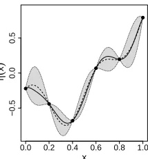
The GP emulator is demonstrated in Figure 1, using a toy model with one input and one output. The plot shows the posterior mean and the 95% posterior credible intervals, highlighting two important features of the emulator:

• The posterior mean,m†_{(.), replicates the training data exactly.}

• The posterior variance is zero at each training data point, so there is no

uncertainty at points where the model has been run.

A consequence of these two features is that the emulator introduces no additional uncertainty into the analysis: the emulator merely fills the gaps between points where the model has been run with probabilistic predictions.

4. Uncertainty analysis using an emulator

The simplest way of using an emulator to carry out an uncertainty analysis is

to use the posterior mean functionm†_{(.) as a direct replacement forη(.) in the}

Monte Carlo procedure detailed in section 2. Once the training data covariance

matrix V has been inverted, m†_{(.) can be evaluated at any input point with}

virtually no computational cost, so the Monte Carlo procedure becomes trivial. However, the problem with this approach is that no account is made for the

extra uncertainty induced by the non-exact approximation ofη(.) bym†(.) at

untried input points.

A better approach is to note that any summary of the uncertainty

distribu-tionS(Y) is itself an uncertain quantity, since it is a function of the unknown

functionη(.). The following Monte Carlo procedure, proposed in [29],

incorpo-rates the uncertainty inη(.) into the analysis:

2. Draw a random function η(j)(.) from the emulator posterior distribution

(eqn. 5) and evaluateη(j)(x1), ...,η(j)(xNx).

3. ObtainSj(Y), the Monte Carlo estimate ofS(Y) using the sample{η(j)(x1), ...,η(j)(xNx)}.

4. Repeat steps 1-2 to obtain a sampleS(Y) ={S1(Y), ..., SNη(Y)}.

5. UseS(Y) to estimate any summary of the distribution ofS(Y).

This Monte Carlo procedure is illustrated in Figure 2, again using a toy model with one input and one output. In the example the aim is to estimate

S(Y) = E[Y], the mean of the uncertainty distribution. Figure 2a shows the

true model output as a function of the input, with the observations that are used to train the emulator. The sample from the input distribution (step 1) and the draws from the emulator posterior (step 2) are shown in Figure 2b. Each draw from the emulator posterior is evaluated at the input sample points

and averaged to give an estimate ofS(Y) (step 3). The collection of estimates,

S(Y), shown in Figure 2c, allows us to estimate summaries of the distribution

of S(Y). For example, the sample median of S(Y), which we denote ˆS(Y),

gives a point estimate ofS(Y), and credible intervals forS(Y) are given by the

quantiles ofS(Y).

We note that the size of the Monte Carlo sample used in this procedure,

Nx, is not limited by computational expense as before. This is because draws

from the emulator posterior distribution are cheap to evaluate. As a result we

can make the Monte Carlo estimate ofS(Y) obtained in step 3 as precise as

we wish, so we consider the error to be effectively zero. In other words, the

uncertainty in the summaryS(Y) is not due to Monte Carlo error, but rather

it stems directly from our uncertainty in the functionη(.).

5. Uncertainty analysis of the FRF

We consider two approaches to analysing the uncertainty distribution of the FRF of the structure using an emulator. Recall that the random variable

Gω represents the FRF at frequency ω, and we consider obtaining arbitrary

summariesS(.) of the distribution ofGω.

5.1. Pointwise analysis

The most straightforward approach is to consider the FRF at a particular

fixed frequencyω∗_{. To obtain the summaryS(G}

ω∗), we use a sequential Monte

Carlo procedure similar to that given above, but in step 3 we obtain the Monte

Carlo estimate ofS(Gω∗) using the sample{η_(j)(x₁), ...,η_(j)(xNx)}. We repeat

steps 1-3 to obtain a sample S(Gω∗) = {S₁(Gω∗), ..., SNη(Gω∗)}, from which

we summarise the distributionS(Gω∗). In particular, we use the median of the

sampleS(Gω∗), denoted ˆS(Gω∗), as a point estimate ofS(Gω∗).

If we are interested in the FRF over a range of frequencies Ω = [ω1, ω2],

we choose a finite number of representative valuesω∗

and apply the above procedure at each representative value. We refer to this approach as a pointwise analysis.

A drawback of a pointwise analysis is that a plot of summaries ofS(Gω∗

1), ..., S(Gω∗Nω)

may be misleading. Suppose, for example, that we chooseS(Gω∗) to be the

up-per 95% quantile ofGω∗. It would be natural to compute ˆS(Gω∗

1), ...,Sˆ(Gω∗Nω),

and to interpolate these values with a curveC0.95. It would then be tempting

and to interpret C0.95 as an estimate of the upper 95% uncertainty bound on

the collection of all the possible FRFs that can be obtained from the FE model. This interpretation would be wrong, though, since the FRF arising from a

par-ticular input pointxcould lie belowC0.95 at one frequencyωi∗ but aboveC0.95

at a different frequencyω∗

j. Thus there is no guarantee that any FRF will lie

belowC0.95 at allω∈Ω.

A further drawback of a pointwise analysis is that a summary ofGω∗ such

as the median,S0.5(G∗ω), which we might expect to give us a central estimate

of the FRF, may bear little resemblance to any actual FRF when calculated

pointwise. In particular, S0.5(G∗ω) will usually be finite for all values of ω∗,

but we know thatG(ω) (computed, as we do here, for an undamped structure)

goes to infinity at ω =

q

ˆ

ki/mˆi for each i = 1, ..., nmodes. This property is

demonstrated in the application in section 6.

5.2. Uncertainty envelope by kernel density estimation

An alternative to the pointwise analysis is to obtain anuncertainty envelope.

For some fixedα∈[0,1], we define an uncertainty envelope to be a set

Eα={(ω, G(ω,y))∈R2:ω∈Ω,y∈R}, (6)

whereR is a subset of modal parameter space such that P r[y∈R] =α. The

uncertainty envelope has the property that the probability thatGωlies outside

ofEαfor some ω∈Ω is 1−α.

Equation (6) does not define a unique uncertainty envelope, since there are

many regions R with the property P r[y ∈ R] = α. We propose choosing R

to be the highest probability density (HPD) region of modal parameter space,

so that for anyy1 ∈R and y2 ∈/ R, pY(y1) ≥pY(y2). We call this the HPD

α-envelope. We note that the HPD region of modal parameter space is not

necessarily connected, so the HPDα-envelope could potentially have ‘holes’ in

it. To simplify the problem, we conservatively estimate the HPDα-envelope as

being the region enclosed by the functions

ℓα(ω) = min

y∈R{G(ω;y)},

uα(ω) = max

y∈R{G(ω;y)}.

In other words we obtain the outer bounds of the uncertainty envelope but ignore any holes in the interior.

A difficulty in calculating the bounds of the HPDα-envelope is that we do

pY(y) using a kernel density estimate (KDE) [30] of a Monte Carlo sample. As before, we use evaluations of the emulator to provide a sequence of Monte Carlo estimates. The algorithm is as follows.

1. Choose a set of representative values{ωi∈Ω :i= 1, ..., Nω}.

2. Draw a sample{x1, ...,xNx} from the input distributionF(x).

3. Draw a random function η(j)(.) from the emulator posterior distribution

(eqn. 5) and evaluateYj ={y

(j) 1 , ...,y

(j)

Nx}, where for i= 1, ..., Nx,y

(j)

i =

η(j)(xi).

4. Obtain ˆp(_Yj)(.), the KDE of the sampleYj.

5. Let Pj ={y(j) ∈ Yj : ˆp

(j) Y (y(

j)_{) ≥ p}∗_{}, where p}∗ _{is the largest number}

such thatPNx

i=1I[ˆp (j) Y (y

(j)

i )≥p∗]> N α.

6. Let ℓ(j) _{be the linear interpolation of the set {(ω}

i,miny∈Pj{G(ωi;y)}) :

i= 1, .., Nx}, and letu(j)be the linear interpolation of the set{(ωi,maxy∈Pj{G(ωi;y)}) :

i= 1, .., Nx}.

7. Let ˆEα(j)be the region of Ω×Renclosed byℓ(j) andu(j).

8. Repeat steps 3-7 to obtain a sampleEα={Eˆ

(1) α , ...,Eˆ

(Nη)

α }

We summarise the sample Eα to obtain an estimate and credible intervals for

the uncertainty envelopeEα. Note that if we chooseα= 0 then this algorithm

returns an estimate of the FRF corresponding to the mode of the uncertainty distribution, as it should.

The HPDα-envelope algorithm is illustrated in Figure 3. In the illustration

there are two inputs x = (x1, x2)T with a uniform distribution, from which

a sample is taken (step 2; Figure 3a). This sample is mapped into modal parameter space by a draw from the emulator posterior (step 3). The KDE of the sample in modal parameter space is used to rank the points according to

their probability density, and the top 100α% are selected (steps 4-5; Figure 3b).

The FRF is computed for each selected point, and the collection of FRFs is used to construct the envelope (steps 6-7; Figure 3c). The procedure is repeated with different draws from the emulator posterior, and each draw results in a different

envelope. The collection of envelopes shows us the uncertainty inEα induced

by only running the FE model at a limited number of input configurations. A disadvantage of the uncertainty envelope approach is that, given a

point-wise analysis, carried out at the α level and at Nω > 1 discrete frequencies,

Eα will be wider than at least one of the pointwise intervals. This is because

the probability of the FRF lying in every pointwise uncertainty interval

simul-taneously is less thanα. Therefore, if interest is only in the FRF at individual

Fuselage length (mm) 1500

Wingspan (mm) 2000

Fuselage thickness (mm) 50

Tail tip massx1 (kg) 0.4 - 0.6

Wingtip massx2 (kg) 0.16 - 0.24

Wing trailing edge thicknessx3(mm) 10.4 - 11.6

Wing leading edge / end plate thicknessx4(mm) 9.5 - 10.5

Young’s modulusx5 (GPa) 64.8 - 79.2

Density (kg/m3_{) 2700}

Poisson’s ratio 0.34

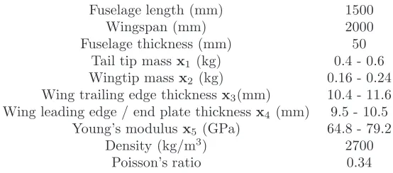
Table 1: Parameters used for the Garteur SM-AG-19 testbed FE model

6. Application

The aircraft model of the Garteur benchmark problem was designed by the Garteur Structures and Materials Action Group 19 (SM-AG-19) to evaluate ground vibration test techniques [31]. The testbed has since been used for a variety of benchmarking and case study problems in structural dynamics, such as FE model updating [32], and fuzzy FE [6]. In the present study, an FE representation of the testbed is used to explore the effectiveness of the proposed statistical emulator approach to uncertainty analysis.

The FE model is based upon thegartfe model included in the Matlab

Struc-tural Dynamics Toolbox (www.sdtools.com). In the physical testbed, a con-strained layer damping treatment is applied to the trailing edge of the wings to increase the structural damping. However, for the present study the structural damping is neglected so as to focus on the undamped FRF predictions that arise directly from the modes of vibration that can be calculated from the FE model.

Meanwhile, five parameters of the FE model, denoted xT _{= (x}

1, ..., x5), are

chosen to be uncertain, with a uniform distribution over a hypercuboidal input space. The resulting physical parameters of the model are listed in Table 1. In practice, such uncertainties may arise due to unknown parameters during the iterative design process, manufacturing inaccuracies/variabilities, or changes in operating conditions. However, for the purposes of the present study the choice of which parameters are uncertain (and their distributions) is somewhat arbi-trary.

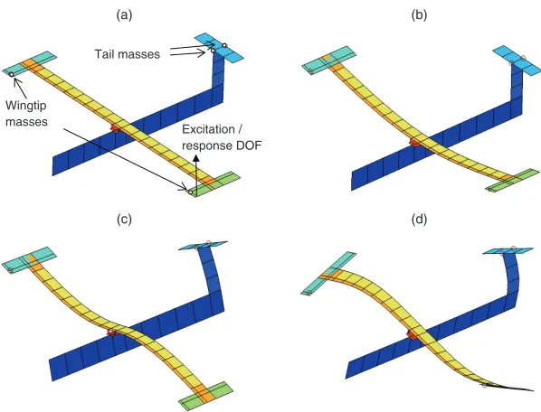
The model structure and resulting modes of vibration are illustrated in Fig-ure 4. In order to consider the FRF of the structFig-ure, a single degree of freedom of the FE model is selected as shown in 4a, and the effective modal mass (kg) and stiffness (N/m) obtained for each of the first 3 structural modes of

vibra-tion. These are referred to as ( ˆm1,ˆk1,mˆ2,kˆ2,mˆ3,ˆk3). The effective mass of

the rigid-body modes of vibration, ˆmrig, was also obtained in order to obtain

mass-dominated receptance FRFs as would be expected for the freely-suspended

structure. The combined output vector isyT _{= ( ˆm}

6.1. Building and validating the emulator

We compare four metamodels for the FE model:

• GPM V: A multivariate GP emulator using the LMC covariance function.

• GPind: A collection of seven independent univariate GP emulators, one

for each output.

• RSlin: A collection of seven independent linear response surfaces. Each

linear RS is a first degree polynomial with pairwise interactions, of the

formy=α0+P5i=1αixi+Pj≥iβijxixj.

• RSquad: A collection of seven independent quadratic response surfaces.

Each quadratic RS is a second degree polynomial with pairwise first degree

interactions of the formy=α0+P5i=1αixi+Pj>iβijxixj.

To train the metamodels we use n = 50 runs of the FE model in a Latin

hypercube design that covers the input space. We also have available a further 20 runs of the FE model, distinct from the training data, that we use to test our emulator. We predict the outputs of the test data using the metamodels.

We find that the predictions of ˆmrig have close to zero error for all four

metamodels. This is because ˆmrig is a very smooth and almost linear function

of the input parameters that correspond to physical masses and dimensions (i.e.

parametersx1 tox4).

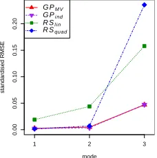
To assess the accuracy of the metamodels in predicting the other outputs we compute the standardised RMS prediction error for each structural mode of vibration as

RM SEj=

v u u u t

20

X

i=1





e(_mˆi)_j rmˆj





2

+





e(ˆ_ki_j)

rˆ_kj





2

, (7)

where e(m_ˆi)j and e

(i) ˆ

kj are the prediction errors for modal parameters ˆmj and ˆkj

respectively, andrmˆj andrˆkj are the ranges of the validation data values for ˆmj

and ˆkj respectively. The standardised RMS prediction errors are compared in

Figure 5, and the relative accuracies of the metamodels are illustrated further in

Figure 6, where we plot validation data and predictions in ( ˆmi,kˆi) cross-sections

of the output space. We see that the prediction accuracies ofGPM V andGPIN D

are almost identical for all three modes. For modes 1 and 2,RSquadand the GP

emulators have very similar RMSEs, which are relatively small compared to the

RMSE ofRSlin. For mode 3 RSquad has worse predictions thanRSlin, while

the GP emulators do better than both the RS metamodels. This suggests that the response of the FE model is non-linear for all modes, and non-quadratic

for mode 3, so the response surfaces we have chosen are not adequate. RSquad

does worse than RSind because, with 31 polynomial coefficients to estimate

are nonparametric, so are better able to adapt to non-linear models than the response surfaces.

Figure 7 shows ( ˆmi,kˆi) cross-sections of the output space, zoomed in on a

single validation point. Also shown in these plots are 95% highest posterior density credible regions for the GP emulator predictions, calculated marginally

for each pair of outputs ( ˆmi,ˆki). These credible regions are ellipses that

repre-sent the joint predictive uncertainty in each pair of modal parameters. Here we see that the main difference between the two GP emulators is in the shape of

the credible regions, most notably in mode 4. GPIN D considers ˆmi and ˆki to

be independent, so its credible regions are ellipses are orientated with the

coor-dinate axes. GPM V, on the other hand, accounts for dependency between ˆmi

and ˆki, so its credible regions are ellipses orientated in the direction of greatest

uncertainty. Consequently, the credible regions ofGPM V better reflect the joint

uncertainty in the modal parameters than do the credible regions of GPIN D.

The advantage of this will be be seen subsequently.

We have demonstrated here that the GP emulators have overall better pre-diction accuracy than the linear and quadratic RS metamodels. They also have the advantage of quantifying the uncertainty in their predictions. We there-fore drop the RS metamodels, using just the GP emulators for the subsequent analyses.

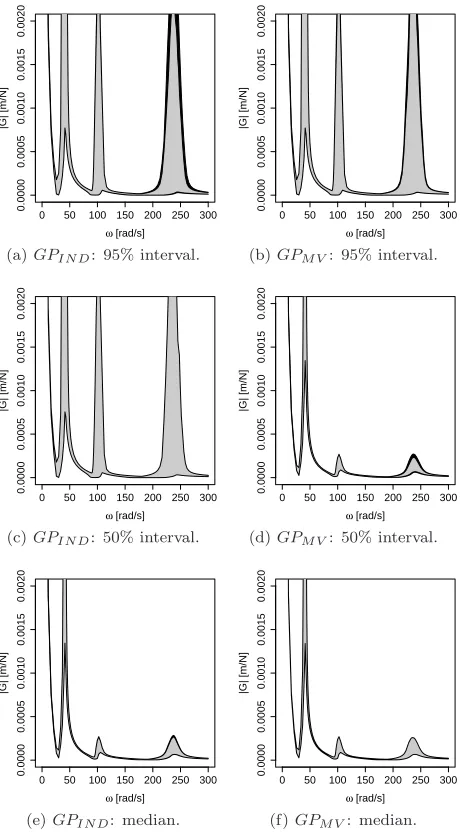
6.2. Pointwise uncertainty analysis

We carry out a pointwise uncertainty analysis of the FRF using the method detailed in section 5.1 with each of the GP emulators in turn. Figure 8 shows the estimates of the median and the 50% and 95% equal-tail uncertainty

inter-vals, calculated pointwise for 100 values ofω spanning the range [0,300]. We

see that the 95% credible intervals for the median and the bounds on the

un-certainty intervals are wider withGPIN Dthan withGPM V, showing that using

a multivariate GP rather than independent univariate GPs results in less

un-certainty in the estimate of the distribution ofGω. The reason for this is that

when the model parameters are combined in the calculation of the FRF, the lack of covariance structure in the independent emulators results in an artificial inflation of the FRF variance.

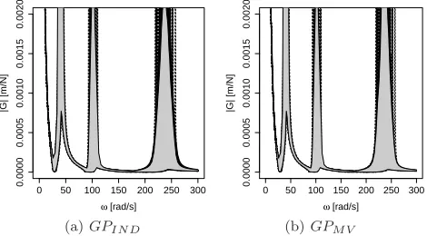
The drawbacks of a pointwise analysis that we discuss in section 5.1 are shown in Figure 9, where we impose the FRFs arising from all 70 evaluations of the FE model that we have available (i.e. both the training and validation data) onto the 95% pointwise equal-tail uncertainty intervals. A total of 63 of these

FRFs fall outside of the interval for some value of ω, demonstrating that the

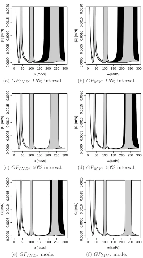
6.3. Uncertainty envelope analysis

Figure 10 shows estimated HPD uncertainty envelopes from each of the two

GP emulators at the levelsα= 0,0.5,0.95. (Recall that the HPD uncertainty

envelope atα= 0 corresponds to the FRF at the mode of the uncertainty

dis-tribution.) The 95% credible intervals for bounds on the uncertainty envelopes

are considerably wider withGPIN D than with GPM V, again because ignoring

the covariance structure results in inflation of the FRF variance. Indeed, the

credible intervals with GPIN D for the 95% uncertainty envelope are so wide

that we would probably conclude that further evaluations of the FE model are required in order to reduce the emulator induced uncertainty to an acceptable

level. WithGPM V, however, the same credible intervals are much smaller and

the extra evaluations may not be required.

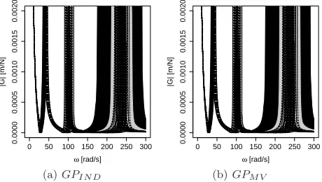
As we expect, the HPD uncertainty envelopes are wider than the interpolated pointwise intervals corresponding to the same probability levels. In Figure 11 we see that all of the FRFs arising from the emulator training and validation data are fully contained within the 95% HPD uncertainty envelope, demonstrating that the uncertainty envelope gives a better overall picture of the region in which we expect to find the FRF.

7. Conclusions

The contribution of this paper is twofold. First, a probabilistic method for quantifying uncertainty in an FRF of a structure is proposed. It is well known that a pointwise analysis (in which an independent uncertainty interval for the FRF is calculated at a finite number of frequencies) can give misleading informa-tion about the FRF as whole. The present study has developed an alternative uncertainty envelope approach, in which an envelope function corresponding to the region of highest probability density in the modal parameter space is calcu-lated. The uncertainty envelope tends to be wider than the corresponding set of pointwise intervals, but has the advantage that it gives a true representation of uncertainty about the location of the entire continuous FRF within a given range of frequencies.

The second contribution of this paper is to introduce the multivariate GP emulator as a tool for performing such probabilistic uncertainty analyses. In the early stages of development of the SFE method it was considered adequate to compute low-order statistics of the variables of interest, but uncertainty analysis for FE methods has become increasingly sophisticated in recent times. The cur-rent state-of-the-art requires estimates of more complex quantities such as mea-sures of reliability, which often can only be computed via Monte Carlo methods. The GP emulator approach introduced in this paper is ideally suited to such applications, since traditional Monte Carlo methods are usually prohibitively expensive in large FE models. The GP emulator has two distinct advantages over other types of metamodel:

• The GP emulator is a form of nonparametric regression that exactly

output at input points where the FE model has been run.

• The Bayesian approach means that the uncertainty about the output at

new input points is quantified and propagated through the rest of the analysis, giving credible intervals for the bounds on the pointwise intervals and the uncertainty envelope.

In a practical example we have demonstrated that GP emulators can give more accurate predictions than linear and quadratic response surfaces. We have also demonstrated that a multivariate GP emulator is better at quantifying uncertainty in multiple outputs than a collection of independent univariate GP emulators. This is because there are dependencies between the outputs, and modelling the uncertainties in them jointly results in a significant reduction in the uncertainty that is propagated through the subsequent analyses. As such, we have shown the multivariate GP emulator to be a very useful tool in the study of multiple output FE models. Further work is needed to extend this approach to consider the problems of overlapping modes of vibration, and uncertain structural damping.

Acknowledgements

This research is part of the ‘Managing Uncertainty in Complex Models’ (MUCM) project, funded by Research Councils UK under its Basic Technology programme, and received support from the EPSRC grants ‘Uncertainty Propa-gation in Structures, Systems and Processes’ (EP/D078601/1) and ‘Bridging the Gaps’ (EP/E01867X/1). The authors thank the other members of the MUCM team for helpful comments.

References

[1] R. Ghanem, P. Spanos, Stochastic finite elements: a spectral approach, Dover Publications, Mineola N.Y., 2003.

[2] B. Lallemand, A. Cherki, T. Tison, P. Level, Fuzzy modal finite element analysis of structures with imprecise material properties, Journal of Sound and Vibration 220 (1999) 353–365.

[3] G. Plessis, B. Lallemand, T. Tison, P. Level, Fuzzy modal parameters, Journal of sound and vibration 233 (2000) 797–812.

[4] L. Hinke, F. Dohnal, B. Mace, T. Waters, N. Ferguson, Component mode synthesis as a framework for uncertainty analysis, Journal of Sound and Vibration 324 (2009) 161–178.

[6] H. De Gersem, D. Moens, W. Desmet, D. Vandepitte, A fuzzy finite element procedure for the calculation of uncertain frequency response functions of damped structures: Part 2–Numerical case studies, Journal of sound and vibration 288 (2005) 463–486.

[7] A. O’Hagan, C. Buck, A. Daneshkhah, J. Eiser, P. Garthwaite, D. Jenkin-son, J. Oakley, T. Rakow, Uncertain judgements: eliciting experts’ proba-bilities, John Wiley, Chichester, 2006.

[8] J. Hammersley, D. Handscomb, Monte carlo methods, Taylor & Francis, 1964.

[9] E. El Tabach, L. Lancelot, I. Shahrour, Y. Najjar, Use of artificial neural network simulation metamodelling to assess groundwater contamination in a road project, Mathematical and Computer Modelling 45 (2007) 766–776.

[10] H. Drucker, C. Burges, L. Kaufman, A. Smola, V. Vapnik, Support vector regression machines, Advances in neural information processing systems (1997) 155–161.

[11] L. Wang, S. GmbH, N. Springer, Support Vector Machines: theory and applications (2005).

[12] T. Lew, A. Spencer, F. Scarpa, K. Worden, A. Rutherford, F. Hemez, Identification of response surface models using genetic programming, Me-chanical Systems and Signal Processing 20 (2006) 1819–1831.

[13] J. Dejean, G. Blanc, Managing uncertainties on production predictions using integrated statistical methods, in: Society of Petroleum Engineers Annual Technical Conference and Exhibition.

[14] A. Rutherford, D. Inman, G. Park, F. Hemez, Use of response surface meta-models for identification of stiffness and damping coefficients in a simple dynamic system, Shock and Vibration 12 (2005) 317–331.

[15] A. O’Hagan, Curve fitting and optimal design for prediction, Journal of the Royal Statistical Society. Series B 40 (1978) 1–42.

[16] A. G. Journel, C. J. Huijbregts, Mining Geostatistics, Academic Press, 1978.

[17] N. Cressie, Statistics for Spacial Data, John Wiley, 1991.

[18] C. E. Rasmussen, C. K. I. Williams, Gaussian Processes for Machine Learn-ing, MIT Press, 2006.

[20] M. Morris, T. Mitchell, D. Ylvisaker, Bayesian design and analysis of com-puter experiments: use of derivatives in surface prediction, Technometrics (1993) 243–255.

[21] S. Conti, A. O’Hagan, Bayesian emulation of complex multi-output and dynamic computer models, Journal of statistical planning and inference 140 (2010) 640–651.

[22] J. Rougier, Efficient emulators for multivariate deterministic functions, Journal of Computational and Graphical Statistics 17 (2008) 827–843.

[23] M. Kennedy, C. Anderson, A. O’Hagan, M. Lomas, I. Woodward, J. Gosling, A. Heinemeyer, Quantifying uncertainty in the biospheric car-bon flux for England and Wales, Journal of the Royal Statistical Society: Series A(Statistics in Society) 171 (2008) 109–135.

[24] T. E. Fricker, J. Oakley, N. M. Urban, Multivariate Emulators with Non-separable Covariance Structures (2010). MUCM Technical Report.

[25] H. Wackernagel, Multivariate Geostatistics, Springer, 1995.

[26] M. Goulard, M. Voltz, Linear coregionalization model: Tools for estimation and choice of cross-variogram matrix, Journal Mathematical Geology 21 (1992) 269–286.

[27] A. E. Gelfand, A. M. Schmidt, S. Banerjee, C. F. Sirmans, Nonstationary multivariate process modelling through spatially varying coregionalization, Test 13 (2004) 1–50.

[28] M. D. McKay, R. J. Beckman, W. J. Conover, A comparison of three methods for selecting values of input variables in the analysis of output from a computer code, Technometrics 21 (1979) 239–245.

[29] J. E. Oakley, A. O’Hagan, Bayesian inference for the uncertainty distribu-tion of computer model outputs, Biometrika 89 (2002) 769–784.

[30] B. Silverman, Density estimation for statistics and data analysis, Chapman & Hall/CRC, 1998.

[31] E. Balmes, J. Wright, GARTEUR group on ground vibration testing: re-sults from the test of a single structure by 12 laboratories in Europe, in: Proceedings of the International Modal Analysis Conference, Orlando.

0.0 0.2 0.4 0.6 0.8 1.0

−0.5

0.0

0.5

x

η

(

x

)

Figure 1: Illustration of an emulator. Depicted are the true function (solid line), the training data (bullets), the posterior mean (dotted line passing through the data points) and the 95% posterior credible intervals (grey regions enclosed by dashed lines).

0.0 0.2 0.4 0.6 0.8 1.0

−0.5

0.0

0.5

x

η

(

x

)

(a)

0.0 0.2 0.4 0.6 0.8 1.0

−0.5

0.0

0.5

x

η

(

x

)

(b)

−0.06

−0.08

−0.10

mean

(c)

Figure 2: Illustration of the Monte Carlo procedure for uncertainty analysis using an emulator. (a) True function with emulator training data. (b) Sample from the input distribution (crosses and dotted grey vertical lines) and four

draws from the emulator posterior (dashed black lines). (c) Estimates ofS(Y) =

E[Y], calculated using each of the realisations (plotting symbols correspond to

those in (b)). The true value of S(Y) =E[Y] is shown by the solid circle and

x1

x2

(a)

m^i

k

^ i

(b)

frequency

|G|

(c)

Figure 3: Illustration of the HPDα-envelope algorithm. (a) Sample from the

input space distribution. (b) Sample mapped to modal parameter space using a single draw from the emulator posterior. Black dots are the points identified as having the highest probability density. (c) FRFs corresponding to each of the black points in (b) (solid lines), with the resulting uncertainty envelope (dashed line).

(a) (b)

(c) (d)

Wingtip masses

Tail masses

Excitation / response DOF

0.00 0.05 0.10 0.15 0.20 mode standardised RMSE

1 2 3

G PM V

G Pi nd

R Sl i n

R Squad

Figure 5: Standardised RMS prediction errors for each structural mode of vi-bration.

3.6 3.7 3.8 3.9 4.0 4.1

6.0

6.5

7.0

7.5

8.0

m^1 [kg]

k

^×1

10

−

3 [N/m] true

G PM V

G Pi nd

R Sl i n

R Squad

(a) Mode 1

12.4 12.8 13.2 13.6

120 130 140 150 160 170

m^2 [kg]

k

^×2

10

−

3 [N/m]

(b) Mode 2

0 2 4 6 8

0 100 200 300 400 500

m^3 [kg]

k

^×3

10

−

3 [N/m]

(c) Mode 3

Figure 6: Predictions of validation points. Depicted are ( ˆmi,ˆki) cross-sections

of the output space, comparing the four metamodels.

3.81350 3.81354 3.81358 3.81362

6.845

6.855

6.865

6.875

m^

1 [kg]

k

^×1

10

−

3 [N/m] true

G PM V

G Pi nd

R Sl i n

R Squad

(a) Mode 1

12.579 12.581 12.583

140.80

140.90

141.00

141.10

m^

2 [kg]

k

^×2

10

−

3 [N/m]

(b) Mode 2

3.0 3.1 3.2 3.3 3.4 3.5 3.6

170 180 190 200 210 m^

3 [kg]

k

^×3

10

−

3 [N/m]

(c) Mode 3

Figure 7: Prediction of a typical validation point. Depicted are ( ˆmi,ˆki)

cross-sections of the output space, comparing the four metamodels. Light grey

re-gions: 95% credible regions forGPIN D. Dark grey regions: 95% credible regions

0 50 100 150 200 250 300

0.0000

0.0005

0.0010

0.0015

0.0020

ω [rad/s]

|G| [m/N]

(a)GPI N D: 95% interval.

0 50 100 150 200 250 300

0.0000

0.0005

0.0010

0.0015

0.0020

ω [rad/s]

|G| [m/N]

(b)GPM V: 95% interval.

0 50 100 150 200 250 300

0.0000

0.0005

0.0010

0.0015

0.0020

ω [rad/s]

|G| [m/N]

(c)GPI N D: 50% interval.

0 50 100 150 200 250 300

0.0000

0.0005

0.0010

0.0015

0.0020

ω [rad/s]

|G| [m/N]

(d)GPM V: 50% interval.

0 50 100 150 200 250 300

0.0000

0.0005

0.0010

0.0015

0.0020

ω [rad/s]

|G| [m/N]

(e)GPI N D: median.

0 50 100 150 200 250 300

0.0000

0.0005

0.0010

0.0015

0.0020

ω [rad/s]

|G| [m/N]

(f)GPM V: median.

Figure 8: Pointwise analysis. Left panels correspond to GPIN D; right

pan-els correspond toGPM V. (a)-(d): 95% and 50% pointwise uncertainty intervals

0 50 100 150 200 250 300

0.0000

0.0005

0.0010

0.0015

0.0020

ω [rad/s]

|G| [m/N]

(a)GPI N D

0 50 100 150 200 250 300

0.0000

0.0005

0.0010

0.0015

0.0020

ω [rad/s]

|G| [m/N]

(b)GPM V

0 50 100 150 200 250 300

0.0000

0.0005

0.0010

0.0015

0.0020

ω [rad/s]

|G| [m/N]

(a)GPI N D: 95% interval.

0 50 100 150 200 250 300

0.0000

0.0005

0.0010

0.0015

0.0020

ω [rad/s]

|G| [m/N]

(b)GPM V: 95% interval.

0 50 100 150 200 250 300

0.0000

0.0005

0.0010

0.0015

0.0020

ω [rad/s]

|G| [m/N]

(c)GPI N D: 50% interval.

0 50 100 150 200 250 300

0.0000

0.0005

0.0010

0.0015

0.0020

ω [rad/s]

|G| [m/N]

(d)GPM V: 50% interval.

0 50 100 150 200 250 300

0.0000

0.0005

0.0010

0.0015

0.0020

ω [rad/s]

|G| [m/N]

(e)GPI N D: mode.

0 50 100 150 200 250 300

0.0000

0.0005

0.0010

0.0015

0.0020

ω [rad/s]

|G| [m/N]

(f)GPM V: mode.

Figure 10: Uncertainty envelope analysis. Left panels correspond to GPIN D;

right panels correspond to GPM V. (a)-(d): Estimated HPD uncertainty

en-velopesE0.95andE0.5 (grey regions) and 95% credible intervals for the bounds

on those envelopes (black regions). (a)-(b): 95% credible intervals for the

0 50 100 150 200 250 300

0.0000

0.0005

0.0010

0.0015

0.0020

ω [rad/s]

|G| [m/N]

(a)GPI N D

0 50 100 150 200 250 300

0.0000

0.0005

0.0010

0.0015

0.0020

ω [rad/s]

|G| [m/N]

(b)GPM V