promoting access to White Rose research papers
White Rose Research Online [email protected]
Universities of Leeds, Sheffield and York
http://eprints.whiterose.ac.uk/
This is an author produced version of a paper published in Medical Decision Making.
White Rose Research Online URL for this paper:
Published paper
Strong, M., Oakley, J. (2011) Bayesian inference for comorbid disease state risks using marginal disease risks and correlation information from a separate source, Medical Decision Making, 31 (4), pp. 571-581
Bayesian Inference for Comorbid Disease State
Risks Using Marginal Disease Risks and
Correla-tion InformaCorrela-tion from a Separate Source
Mark Strong1 and Jeremy E. Oakley2
1. School of Health and Related Research, University of Sheffield, Regent Court,
30 Regent Street, Sheffield, S1 4DA, UK
2. Department of Probability and Statistics, University of Sheffield, Hicks
Build-ing, Hounsfield Road, Sheffield, S3 7RH, UK
Funding. MS is supported by a UK Medical Research Council Health Services
Re-search / Health of the Public reRe-search training fellowship [grant number G0601721].
Address correspondence to Mark Strong, ScHARR, Regent Court, Sheffield, S1
This is the pre-publication, author-produced version of a manuscript published in
Medical Decision Making: Strong M, Oakley JE. Bayesian inference for comorbid
disease risks using marginal disease risks and correlation information from a
sep-arate source. Med Decis Making. 2011 Jul-Aug;31(4):571-81. Epub 2011 Jan 6.
doi: 10.1177/0272989X10391269.
Available at http://mdm.sagepub.com/content/31/4/571.
Disclaimer: “This version does not include post-acceptance editing and
format-ting. Medical Decision Making is not responsible for the quality of the content
or presentation of the author-produced accepted version of the manuscript or of
any version that a third party derives from it. Readers who wish to access the
definitive published version of this manuscript and any ancillary material related
to this manuscript (correspondence, corrections, editorials, linked articles, etc.)
should go to http://mdm.sagepub.com/. Those who cite this manuscript should
ABSTRACT
Background. Public health interventions are increasingly being evaluated for
their cost-effectiveness. Such interventions act ‘upstream’ on the determinants of
ill health and therefore may reduce the incidence of several diseases. In this case
the risks of the separate diseases are likely to be correlated at the individual level,
and considerable comorbidity may be present. An economic evaluation should
take this comorbidity into account, but estimates of the risks and intervention
effects may only be available separately for each disease. This paper proposes a
method for combining marginal disease risks and treatment effects with correlation
information from a separate source in order to estimate comorbid disease risks and
treatment effects.
Method. A case study is presented based on a physical activity cost-effectiveness
model. The correlation between the risk of coronary heart disease, stroke and
di-abetes is estimated from cross sectional data using a Bayesian multivariate probit
model. This information is then combined with disease specific marginal baseline
risks and intervention effects to give comorbid disease state risks. The expected
numbers of QALYs gained through avoiding the comorbid states is estimated from
disease specific utility data under a range of assumptions. Finally, the
incremen-tal benefit of physical activity is calculated under these utility assumptions. The
difference in effectiveness of the intervention due to its impact on reducing or
increasing the disease risk correlations is explored in a sensitivity analysis.
Results. If comorbidity is not taken into account, total benefit is overestimated
compared with all scenarios in which the comorbidity is included in the model.
The overestimation is greatest when physical activity is assumed to reduce disease
INTRODUCTION
The motivation for this paper is the problem of estimating the risks of comorbid
disease states when only single disease risk estimates are available from empirical
studies. We initially recognised this difficulty in the context of parametrizing a
cost-effectiveness model for a ‘public health’ physical activity promoting
interven-tion that was expected to have an impact on the risk of several different diseases.
We expect though that the problem of finding comorbid disease state estimates,
and our proposed solution, will be applicable in many different health economic
modeling contexts, not just those classified as public health.
Public health interventions are generally directed ‘upstream’ at the determinants
of ill health, and as such are commonly expected to have an impact on more than
one disease.1 An example of an upstream determinant of ill health is an
individ-ual’s level of physical activity, with a sedentary lifestyle being associated with a
range of diseases, including stroke, diabetes and coronary heart disease (CHD). If
we wish to evaluate the cost-effectiveness of a physical activity promoting
inter-vention, we will therefore need to take account of the impact of the intervention
on the costs and benefits associated with more than one disease.
The UK National Institute of Health and Clinical Excellence (NICE) has
eval-uated the cost-effectiveness of physical activity promoting interventions as part
of its Public Health Guidance programme.2 In the economic model published in
support of the physical activity guidance,3 four diseases were considered: CHD,
stroke, diabetes and colon cancer, and a choice was made to evaluate the
incre-mental costs and benefits of physical activity promoting interventions separately
for each disease. The total incremental cost and total incremental benefit of the
intervention were then assumed to be the sums, respectively, of the four disease
specific incremental costs and benefits. This approach of summing incremental
costs and consequences calculated separately for a number of diseases is common
to a number of other NICE Public Health guidance economic evaluations,4–6 and
is attractive because evidence required to inform parameter values in the model
effectiveness of the intervention in reducing the risk of thecomorbid disease states (e.g. CHD and diabetes), or on the costs and consequences of those states.
If we assume that the risks and treatment effects for the single disease states in the
above models are marginal risks and treatment effects, then summing the expected
population costs and consequences that relate to the impact of the intervention
on these marginal risks is equivalent to assuming that, where comorbidity exists,
the costs and consequences associated with the separate diseases are additive at
the individual level. To give an example, this means that the cost saved when
an individual person avoids both coronary heart disease (CHD) and a stroke is
assumed to be the same as the sum of the costs saved when one person avoids
CHD and another avoids a stroke. Likewise, the benefit gained by that individual
is assumed to be equal to the sum of the benefits gained when one person avoids
CHD, and another avoids a stroke.
To see why this additive assumption is unlikely to hold for benefits, consider a
simple example in which benefits are measured in life-years gained. Assume an
intervention has the effect of preventing two diseases, A and B. The average age
of death is 60 years for a person with disease A, and 65 years for a person with
disease B. Without disease, the average age of death is 75 years. The number of
life-years gained is 15 for a person avoiding A, and 10 for a person avoiding B. It
is difficult to justify why a person avoiding both A and B would gain 25 years of
life.
Secondly, consider an example in which an intervention has an effect on quality
of life, but not its length, through its effect on two diseases A and B. Health state
utility valuations are used as the measure of quality of life. Let’s imagine that
disease A is associated with a utility weight of 0.7 and disease B with a utility
weight of 0.6, while the state of absence of A and B is associated with a utility
weight of 0.9. Calculating the population expected benefit under the additive
assumption would be equivalent to assuming that a person who avoids both A
and B for one year gains (0.9−0.7) + (0.9−0.6) = 0.5 Quality Adjusted Life Years (QALYs).
quality of life. In the first case a better assumption may be that the number of
life-years gained when a comorbid state is avoided is the same as the number of
life-years gained when avoiding the component disease that has the earliest age of
death. In the second case there are again more compelling models for comorbid
health state utility weights, both for theoretical reasons,7 and based on empirical
data.8 A common assumption is that the utility weight for a joint health state
is the product of the utility weights for the individual component states. In the
same way, costs accruing due to the prevention of multiple diseases are unlikely to be simply additive, and we may envisage a range of more plausible models.
If we do decide to base our analysis on a non-additive assumption regarding the
comorbid costs and consequences, we will need to quantify the risks of these co-morbid disease states under both the intervention and the baseline comparator,
and as stated above it is this requirement that provides the motivation for our
paper. In order to estimate comorbid disease state risks we need to know
some-thing about the degree of co-occurrence (correlation) between the diseases at an
individual level, something that is not obtainable from the disease specific studies
that are usually used to inform baseline disease risks and treatment effects.
Given that we may not be able to find direct estimates for the comorbid
dis-ease state risks in the intervention and comparator groups, our paper proposes
a method for combining estimates of the marginal disease specific baseline risk
and treatment effects with information relating to the correlation between disease
risks derived from an external source. To illustrate our method we have created a
simplified version of the NICE physical activity model as a case study that runs
throughout the paper.
CASE STUDY
Our case study is loosely based on the economic model published as part of the
NICE physical activity guidance.3 For simplicity of illustration we restrict
our-selves to consider only the incremental benefits (in QALYs) of physical activity
ourselves to considering the effect of physical activity on three diseases: CHD,
stroke and diabetes.
The ‘marginal’ economic model
In this section we describe our simplified version of the NICE guidance economic
model and the evidence used to inform the parameter values. We call this the
‘marginal’ model since it is parametrized in terms of the marginal disease risks
and incremental benefits for the three diseases.
We are interested in the incremental health consequences (in QALYs) of the
in-tervention compared with baseline. The model assumes four disease states: well,
CHD, stroke and diabetes. Each state is associated with a population mean
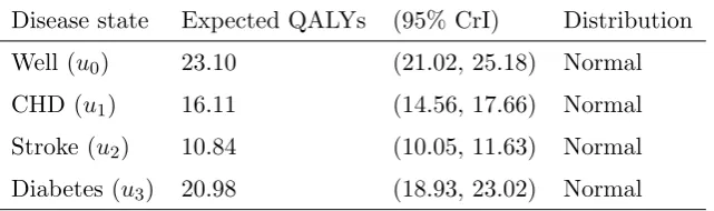
util-ity in QALYs, shown in Table 1. Utilities were derived from data reported in the
[image:8.595.109.430.418.513.2]NICE modeling document.3
Table 1. Utility values in QALYs for marginal disease states
Disease state Expected QALYs (95% CrI) Distribution
Well (u0) 23.10 (21.02, 25.18) Normal
CHD (u1) 16.11 (14.56, 17.66) Normal
Stroke (u2) 10.84 (10.05, 11.63) Normal
Diabetes (u3) 20.98 (18.93, 23.02) Normal
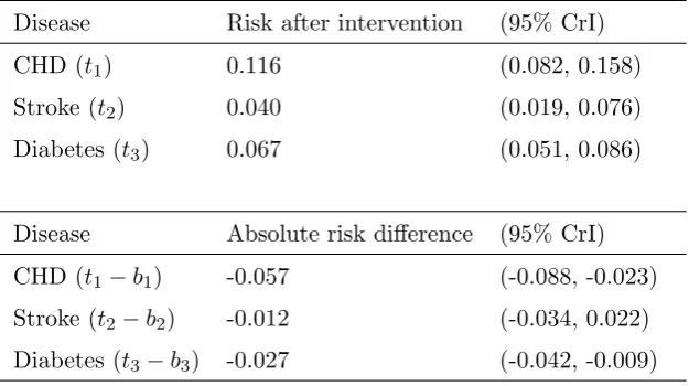
The (baseline) incident risks of CHD, stroke and diabetes in a sedentary
popula-tion, indexed j = 1, . . . ,3, are denoted bj, and the treatment effects (as relative
risks) are denoted RRj (see Table 2). Ideally these estimates would be derived
from studies conducted in populations that are similar to the population of
inter-est. Givenbj andRRj it is then possible to derive estimates for the risks after the
intervention, tj = bj ×RRj, and the absolute risk differences, tj −bj (see Table
Table 2. Baseline risks and treatment effects
Disease Baseline risk (95% CrI) Distribution Study
CHD (b1) 0.172 (0.139, 0.209) Normal Wannamethee21
Stroke (b2) 0.053 (0.046, 0.060) Normal Wolf22
Diabetes (b3) 0.094 (0.085, 0.104) Normal Kriska23
Disease Treatment effect (95% CrI) Distribution Study
CHD (RR1) 0.67 (0.52, 0.86) Lognormal Salonen24
Stroke (RR2) 0.72 (0.37, 1.42) Lognormal Herman25
Diabetes (RR3) 0.71 (0.56, 0.91) Lognormal Manson26
Table 3. Risk after intervention and risk difference
Disease Risk after intervention (95% CrI)
CHD (t1) 0.116 (0.082, 0.158)
Stroke (t2) 0.040 (0.019, 0.076)
Diabetes (t3) 0.067 (0.051, 0.086)
Disease Absolute risk difference (95% CrI)
CHD (t1−b1) -0.057 (-0.088, -0.023)
Stroke (t2−b2) -0.012 (-0.034, 0.022)
Diabetes (t3−b3) -0.027 (-0.042, -0.009)
The marginal model assumes the overall incremental benefit in QALYs, denoted
∆E, is
∆E =
3
X
j=1
(tj −bj)(uj−u0), (1)
where uj is the population mean expected number of QALYs experienced by
someone with disease j. Those who are well have an expected number of QALYs ofu0anduj−u0 is therefore the expected number of QALYs ‘lost’ by an individual
who has disease j.
[image:9.595.108.421.362.537.2]estimated incremental benefit of 0.602 QALYs. This can be interpreted as an
additional 0.602 years of perfect health, or an additionaln×0.602 years of health with a utility weight of n−1. Propagating parameter uncertainty through the model using standard Monte Carlo based probabilistic sensitivity analysis with
10,000 samples leads to a 95% credible interval of 0.114 to 1.005 QALYs. For
the purposes of the uncertainty analysis we assumed normal distributions for the
baseline risks,bj, and benefits in QALYs,uj. For relative risks,RRj, we assumed
lognormal distributions since these are ratio measures bounded at zero.
Problems with the marginal model
The three disease states CHD, stroke and diabetes are clearly not mutually
exclu-sive since it is possible for an individual to have more than one of these diseases;
however, there are no parameters in the model that relate to the risks or utilities
of the comorbid states. By evaluating overall incremental benefit via Equation 1
we are implicitly making the assumption that the benefit of avoiding a comorbid
state (for example, the state of CHD and diabetes) is the sum of the benefits of
avoiding each of the component disease states. If we wish to avoid making this
additive assumption we need to estimate the risks and utilities for the complete
set of mutually exclusive joint disease states, rather than just the marginal risks and single disease specific utilities.
Given three diseases there are 23 = 8 mutually exclusive joint disease states,
including the state of good health. In our example these states are: well, CHD
alone, stroke alone, diabetes alone, CHD and stroke, CHD and diabetes, stroke
and diabetes, and all three diseases. We refer to this set of eight mutually exclusive
disease states as the joint disease states and the parameters that relate to these states are denoted by a superscript ‘∗’. We refer to the four disease states within this set that comprise more than one disease as the comorbid states.
If we are able to estimate parameters for the joint states, our new model for
incremental benefit will be
∆E∗ =
7
X
k=0
wherek indexes the eight mutually exclusive joint disease states (well, CHD alone, stroke alone, diabetes alone, CHD and stroke, CHD and diabetes, stroke and
diabetes, all three diseases), b∗k is the baseline risk of disease state k, t∗k is the intervention risk of disease k, and u∗k is the expected number of QALYs for an individual in disease state k. The disease free state is indexed k = 0.
Equation 2 can be written in the same form as Equation 1 by recognizing the
following. BecauseP7
k=0t ∗
k = 1 and
P7
k=0b ∗
k = 1, this means that
P7
k=0(t ∗
k−b
∗
k) =
0, and therefore that (t∗0−b∗0) = −P7
k=1(t ∗
k−b
∗
k). As a result we can write
∆E∗ =
7
X
k=0
(t∗k−b∗k)u∗k,
=
7
X
k=1
(t∗k−b∗k)u∗k+ (t∗0−b∗0)u∗0,
=
7
X
k=1
(t∗k−b∗k)u∗k−
7
X
k=1
(t∗k−b∗k)u∗0,
=
7
X
k=1
(t∗k−b∗k)(u∗k−u∗0).
Estimating the utilities for the joint disease states (u∗k)
The utility, in QALYs, for a disease state is determined by both length and quality
of life. We assume that we do not have empirical evidence that relates to the mean
length of life for the comorbid states, and nor do we have quality of life data for
the comorbid states. We therefore must model these parameters based on the
length and quality of life data for the single diseases.
As regards length of life we assume that the age of death for an individual who
has more than one disease is the earliest of the ages of death for the single diseases
that make up the individual’s comorbid disease state. As regards quality of life
we explore three models, based on theoretical and empirical arguments in the
literature.7, 8
for the single diseases that make up the comorbid state.
Joint state QALY model 2 - minimum. The quality of life weight for each comorbid state is the minimum of the utility weights for the single diseases that make up
the comorbid state.
Joint state QALY model 3 - additive decrement. The reduction in quality of life weight between the well state and each comorbid state is the sum of the utility
decrements (i.e. the difference in utility weight between well and disease) for the individual diseases that make up the comorbid state.
Note that model 3 differs from the marginal model in that total benefits in QALYs
are assumed to be additive under the marginal model, whereas in model 3 the
additive decrement assumption applies only to quality of life weights. Length of life decrements are not additive under any of the joint state QALY models.
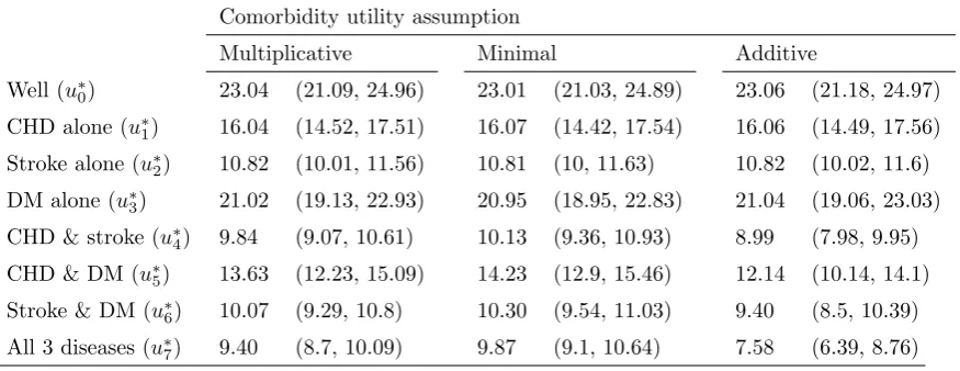
Table 4 shows the estimated utility in QALYs for the eight joint states calculated
[image:12.595.111.549.455.624.2]under these three models.
Table 4. Utility values in QALYs (95% CrI) for joint disease states under models 1-3
Comorbidity utility assumption
Multiplicative Minimal Additive
Well (u∗0) 23.04 (21.09, 24.96) 23.01 (21.03, 24.89) 23.06 (21.18, 24.97)
CHD alone (u∗
1) 16.04 (14.52, 17.51) 16.07 (14.42, 17.54) 16.06 (14.49, 17.56)
Stroke alone (u∗2) 10.82 (10.01, 11.56) 10.81 (10, 11.63) 10.82 (10.02, 11.6)
DM alone (u∗3) 21.02 (19.13, 22.93) 20.95 (18.95, 22.83) 21.04 (19.06, 23.03)
CHD & stroke (u∗4) 9.84 (9.07, 10.61) 10.13 (9.36, 10.93) 8.99 (7.98, 9.95)
CHD & DM (u∗5) 13.63 (12.23, 15.09) 14.23 (12.9, 15.46) 12.14 (10.14, 14.1)
Stroke & DM (u∗6) 10.07 (9.29, 10.8) 10.30 (9.54, 11.03) 9.40 (8.5, 10.39)
All 3 diseases (u∗7) 9.40 (8.7, 10.09) 9.87 (9.1, 10.64) 7.58 (6.39, 8.76)
Estimating the joint disease risks, b∗k and t∗k
We assume that we have estimates of the baseline risks and treatment effects
relevant to our population (we call this dataset A). We do not have information on
the baseline risks and treatment effects for the comorbid disease states since the
studies we have found are disease specific. However, we do have information from
elsewhere that relates to the correlation between our three diseases in the form of
individual level data from a cross sectional study (we call this dataset B). If the
correlation information in dataset B can be combined with the estimates of the
marginal baseline risks and treatment effects in dataset A then we can estimate
the eight joint disease risks we require.
The presence or absence of the three diseases in dataset B represents correlated
binary data. However, describing correlation between binary variables is not
straightforward. The Pearson correlation coefficient will depend on the
popu-lation proportions of the three diseases, and instead of varying between −1 and
+1 as it does for continuous data, will lie on a narrowed interval that is not
sym-metric about 0, potentially making interpretation of the measure difficult. Ideally,
we would like a measure of correlation that is independent of the marginal
popu-lation proportions of the three diseases, and that lies between−1 and +1 for ease
of interpretation.
One solution to this problem is to link the correlated binary outcomes to a latent
variable with a multivariate normal distribution, therefore allowing the
correla-tion structure in the data to be expressed through the covariance matrix of the
multivariate normal distribution. If the covariance matrix is expressed in
corre-lation form, then we have a measure that fulfils both our criteria above. Linking
a binary outcome to an underlying multivariate normal latent variable is an
ex-ample of the use of a multivariate probit model, discussed in detail by Chib and
Greenberg (1998),9 and by Albert and Chib (1993).10
To illustrate the multivariate probit model we first assume that we have data, yij,
on i = 1, . . . , n individuals, relating to the presence or absence of j = 1, . . . ,3 diseases. The binary data yij are linked to the latent variable, denoted zij, via
yij = I(zij > 0), where I(·) is the indicator function, taking value 1 if zij > 0,
and 0 otherwise. The latent variable vector for each individual i is denoted zi =
that they are realizations of a random variable, Zi, with Zi ∼ N3(µ,Σ). Here,
µ = (µ1, µ2, µ3) describes, on the latent continuous scale (i.e. −∞ to +∞), the
marginal disease risks in the cross-sectional study population, and the covariance
matrix Σ models the dependency between the binary disease states. The latent
variable Zi could be envisaged as quantifying an underlying degree of propensity
for each disease on a continuous scale. If the propensity for diseasej exceeds some threshold, then that disease occurs.
Estimating Σ for our case study
We have cross sectional data on 18,553 individuals that relate to the presence or
absence of CHD, stroke and diabetes. These data come from the Health Survey for
England (HSE) 2003.11 The HSE is a large, annually conducted survey of a
rep-resentative sample of the population of England that aims to provide information
on the health status of the population.
We took a Bayesian approach and estimated the correlation between the risks of
CHD, stroke and diabetes from the HSE data using Chib and Greenberg’s
mul-tivariate probit model (see Appendix A). Appendix B shows annotated BUGS
code that we ran in OpenBUGS 3.0.8.12 We placed the following weak priors
on the mean and correlation parameters: µ ∼ N3(0,106I3) and Σ ∼ IW(I3,3),
where I3 is the three dimensional identity matrix andIW is the inverse Wishart
distribution, parametrized in terms of an inverse scale matrix and a number of
degrees of freedom.13 We ran three Markov chains, each with a different set of
ini-tial parameter values. The Brooks-Gelman-Rubin diagnostic suggested adequate
convergence after a burn in of 50,000 samples.14, 15
The samples from the posterior distribution of the parameters of the correlation
matrix, Σ, were highly autocorrelated. The presence of positive autocorrelation
in an MCMC chain increases the number of samples required to achieve some
pre-specified level of accuracy in the estimates of the mean and variance of the
posterior distribution.16 This is because each successive iteration in an
iteration in an uncorrelated chain.
Thinning the chain is sometimes employed to reduce autocorrelation and is
ap-propriate if the size of the sample that can be processed is fixed at some level,
usually due to limited computer memory storage. Given a chain of length N, and a thinned sample set of length n from that chain (i.e. thinning the chain keeping everykthsample wherek = N
n) it is better to base inference on the thinned sample
set of sizen, than on n consecutive samples from the un-thinned chain. However, inferences based on a thinned sample set of size n will always be less accurate than inferences based on the full un-thinned chain of length N.17
We generated a total of 250,000 samples from the three MCMC chains after
burn-in and estimated means and variances for the parameters of the correlation matrix,
Σ, using the whole sample set. We then selected every 25th sample (i.e. 10,000
samples in total) for use within the economic model, given that propagating all
250,000 samples through the economic model in a probabilistic sensitivity analysis
(described below) would have taken a prohibitively long time. Thinning the chain
in this way, rather than simply selecting the first 10,000 samples, reduced the
autocorrelation in the sample set used within the economic model and therefore
increased the accuracy of the probabilistic sensitivity analysis.
The marginal risks calculated from the HSE dataset were 46 per 1000 for CHD,
20 per 1000 for stroke and 33 per 1000 for diabetes, and the correlations between
the disease risks on the latent scale were 0.509 (95% CrI 0.459 to 0.558) for CHD
and stroke, 0.441 (95% CrI 0.391 to 0.490) for CHD and diabetes, and 0.400 (95%
CrI 0.338 to 0.460) for stroke and diabetes.
Combining Σ with marginal risks to calculate joint disease state risks
Once we have estimated Σ we must then combine this correlation information
with the marginal disease risks bj and tj to give the baseline and treated risks
b∗k and t∗k for the k = 0, . . . ,7 joint states. There is no closed form analytical solution to this problem, but the simulation based solution described below is
The marginal risks bj and tj are first transformed onto the latent scale via the
inverse normal cumulative distribution function, Φ−1(·),
µbj = Φ
−1(b
j),
µtj = Φ
−1(t
j).
To obtain the joint disease risks for baseline we draw a large number (i= 1, . . . , m) of samples, zi = (zi1, zi2, zi3), from the tri-variate N3(µb,Σ) distribution, where
µb = (µb1, µb2, µb3). These samples are transformed onto the binary scale via the indicator function yij = I(zij > 0) giving a correlated binary dataset with
marginal disease risks bj, and a correlation structure that reflects the individual
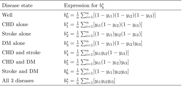
level disease dependence that we require. The joint risks b∗k are obtained from the yij via the expressions in Table 5. The eight joint absolute risks for the
intervention group t∗k are calculated in the same manner. This is done using the same correlation matrix,Σ, as for the baseline risks, or using a different correlation
matrix if there is evidence to support a different dependence structure after the
[image:16.595.110.494.444.618.2]intervention.
Table 5. Expressions for calculating joint disease risks
Disease state Expression for b∗k
Well b∗0 = 1nPni=1[(1−yi1)(1−yi2)(1−yi3)] CHD alone b∗1 = 1nPni=1[yi1(1−yi2)(1−yi3)] Stroke alone b∗2 = 1nPni=1[(1−yi1)yi2(1−yi3)] DM alone b∗3 = 1nPni=1[(1−yi1)(1−yi2)yi3] CHD and stroke b∗4 = 1nPn
i=1[yi1yi2(1−yi3)] CHD and DM b∗5 = 1nPni=1[yi1(1−yi2)yi3] Stroke and DM b∗6 = 1nPni=1[(1−yi1)yi2yi3] All 3 diseases b∗7 = 1nPni=1[yi1yi2yi3]
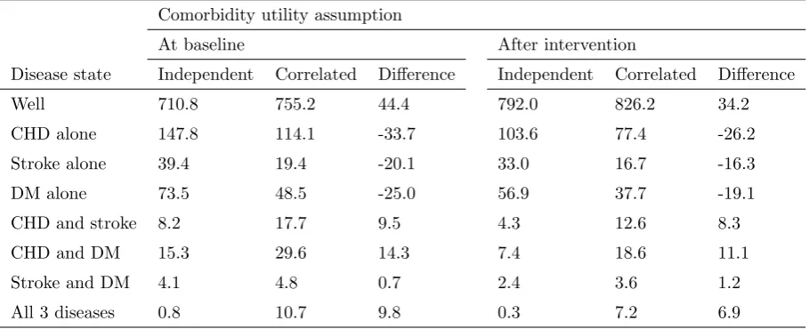
Table 6 shows the estimated absolute risk for each joint disease state at baseline
(no physical activity) and with physical activity (expressed as numbers of cases per
1000 population) under two assumptions: firstly that disease risks are independent
(i.e. that Σ = I3), and secondly that the correlation is the same as that in the
Table 6. Estimated numbers of cases (per 1000 pop) by joint disease outcome
Comorbidity utility assumption
At baseline After intervention
Disease state Independent Correlated Difference Independent Correlated Difference
Well 710.8 755.2 44.4 792.0 826.2 34.2
CHD alone 147.8 114.1 -33.7 103.6 77.4 -26.2
Stroke alone 39.4 19.4 -20.1 33.0 16.7 -16.3
DM alone 73.5 48.5 -25.0 56.9 37.7 -19.1
CHD and stroke 8.2 17.7 9.5 4.3 12.6 8.3
CHD and DM 15.3 29.6 14.3 7.4 18.6 11.1
Stroke and DM 4.1 4.8 0.7 2.4 3.6 1.2
All 3 diseases 0.8 10.7 9.8 0.3 7.2 6.9
The risk of being in either a comorbid state, or in the no disease state, is greater
un-der the correlated risks assumption than unun-der the independence assumption,
re-flecting the positive correlations in risks between all three marginal disease states.
Calculating incremental benefit under a range of scenarios
We explored a range of scenarios in which we combined different assumptions
about disease risk correlation structure with different models for the comorbid
disease states utilities.
In the first three scenarios we considered disease risks to be independent, both
at baseline and after the intervention. In the second set of three scenarios we
considered both baseline and treated risks to be correlated, with the degree of
correlation estimated from the HSE data. Because there may be good reasons for
assuming different correlation structures in the baseline disease risks and treated
risks we wanted to explore two further scenarios. Baseline risks were assumed to
have the same correlation structure as that estimated from the HSE data, but
treated risks were assumed firstly, to have a higher degree of correlation (by a
factor of 10%), and secondly, to have a lesser degree of correlation (by a factor of
For each of the four sets of scenarios we assumed the three models described above
for comorbid disease state utilities: multiplicative, minimal and additive. In each
of the resulting 12 scenarios we calculated the incremental benefit via Equation
2.
Probabilistic sensitivity analysis
In order to conduct a probabilistic sensitivity analysis, uncertainty in the
esti-mates for the baseline risk and treatment effect parameters, as well as for the
correlation matrix, Σ, must be propagated through the model. Because the joint
risk parameters b∗k and t∗k are calculated via simulation, two levels of simulation are required to determine the uncertainty in the model output. See Halpern et al
for a discussion of such nested models.18 Samples are drawn from the posterior
distributions of the parameters uj, bj, RRj and Σin an outer loop, and for each
run of the outer loop, the joint risk parameters b∗k andt∗k are estimated through a large number of runs of an inner, nested, loop. For the purposes of our case study
we drew 10,000 samples from the outer loop parameters, and based each estimate
of b∗k and t∗k on 2,000 inner loop samples.
Results
If the benefits of the intervention are calculated separately for each disease and
then summed (the marginal approach as taken in the NICE models identified in
the introduction,2, 4–6) then the overall incremental benefit calculated via Equation
1 is estimated to be 0.602 (95% CrI 0.114 to 1.005). This marginal approach
overestimates the benefit of the intervention compared with that predicted in all
our twelve scenarios (Table 7). The overestimation is largest when the marginal
approach is compared with the scenario in which the minimal model was used to
estimate utilities of the comorbid states, the baseline risks were correlated, and the
correlation in the risks was reduced after the intervention. The overestimation is
least in the case where the additive decrement assumption was used for comorbid
Table 7. Incremental benefits in QALYs (SE)
Comorbidity utility assumption
Additive
decrement
Minimal Multiplicative
Baseline
risks
Treated
risks
Independent Independent 0.590 (0.220) 0.568 (0.218) 0.573 (0.217)
HSE HSE 0.565 (0.229) 0.519 (0.216) 0.533 (0.220)
HSE HSE+10% 0.573 (0.228) 0.533 (0.215) 0.546 (0.219)
HSE HSE−10% 0.558 (0.229) 0.506 (0.216) 0.522 (0.221)
HSE. Correlation structure estimated from the Health Survey for England data.
In general, the overestimation of the marginal approach will be worst when there
is a high degree of positive correlation between disease risks at baseline which
then weakens after the intervention. To see why, consider the following. A large
positive correlation between diseases at baseline implies that many individuals
who are ill will have more than one disease. If, in the intervention group, the
correlation in disease risk is smaller than in the baseline group, then this implies
that the intervention is protective against the comorbid states, and that many
instances of a comorbid disease state would be avoided if the intervention were
to be implemented. Under the marginal model the value of avoiding a comorbid
state is overvalued, primarily due to the unrealistic assumption of additivity of
life years gained, and it is this overvaluation that leads to the overestimation of
incremental benefit.
DISCUSSION
Our analysis suggests that the marginal approach to modeling the impact of an
intervention on multiple diseases is likely to overestimate the overall benefit, unless
benefits really are additive at an individual level. Even if diseases are assumed to
be independent, the marginal approach will still lead to overestimation of benefit
because the marginal approach assumes an additive decrement of length of life as
will only be avoided if the diseases are mutually exclusive.
The differences between the results of the marginal model and the twelve
alter-native scenarios we present in our case study are modest. However, even small
differences in costs and benefits may be important if the overall cost-effectiveness
is close to the decision threshold. This holds even when credible intervals overlap
since it is the mean incremental costs and benefits that are of primary importance
to the decision maker.19
The ideal approach to modeling cost-effectiveness in the presence of multiple
dis-eases would be to explicitly include parameters that relate to all the possible joint
disease states, and obtain values for these parameters directly from the
litera-ture. It would then be entirely correct to sum costs and benefits over these states
since they would be mutually exclusive. The difficulty is finding estimates of the
baseline risks and treatment effects for the joint states in the literature.
Limitations
Our approach has a number of limitations. Fundamental to the latent variable
formulation is the belief that the correlation structure in a multivariate normal
continuous variable can, for our purposes, meaningfully model the correlation
structure in the multivariate binary disease outcome. Multivariate normality
im-plies that the correlation is independent of the mean marginal disease risks on the
latent scale, but this is not true for the binary disease outcomes, where variances
and covariances are functions of the mean.
If the latent variableZiis considered to have a physical meaning, in that evidence
suggests that each disease state arises when some underlying continuous process
exceeds a threshold, then our approach would seem reasonable on these grounds.
However, if no such physical interpretation for the latent variable exists, then the
variable might be considered instead an artefact, included in order to introduce
into the cost-effectiveness model information about the correlation structure in an
external data set. In this case it may be necessary to consider carefully whether the
are similar enough to those in the studies used to derive the risk estimates in the
model, given the dependence between the correlation and mean in multivariate
binary data.
In our case study the marginal risks of CHD, stroke and diabetes were estimated
as 172 per 1000, 53 per 1000 and 94 per 1000 at baseline (no physical activity),
and as 115 per 1000, 38 per 1000 and 67 per 1000 in those who took exercise.
Both baseline (no physical activity) and intervention (active) disease risks are
somewhat higher in magnitude than the marginal disease risks estimated from
the HSE data, which were 46 per 1000 for CHD, 20 per 1000 for stroke and 33 per
1000 for diabetes. Ideally we would estimate the baseline disease risk correlation
using data from a sedentary population whose marginal disease risks are as close
as possible to the baseline risk estimates we are using to parametrize the economic
model. Likewise, intervention disease risk correlations would ideally be estimated
using data from an active population with marginal disease risks similar to the
intervention group risks used in the economic model.
Lastly, we have been able to estimate the correlation between the disease states
in our model from primary data. These data may not always be available, and
in this case expert elicitation may be considered as an option for learning about
the correlations between disease states. The correlation parameters in our model
essentially represent the correlations in underlying risks of disease, each expressed
on a continuous scale, and their meaning, at least in a qualitative sense, could be
expected to be fairly well understood intuitively. However, eliciting values for the
correlation parameters is likely to be difficult, particularly for cases where there
are more than two disease states.20
Conclusion
This paper presents one approach to synthesizing information relating to disease
risk correlation with marginal risks and treatment effects in order to estimate
joint risks and treatment effects in the absence of direct empirical data. The
dif-ferent assumptions about the correlation between disease risks, and as such has
References
1. NICE. Methods for the development of NICE public health guidance (second
edition). NICE; 2009. Available from: http://www.nice.org.uk/phmethods.
2. NICE. Four commonly used methods to increase physical activity (PH2).
NICE; 2006. Available from: http://guidance.nice.org.uk/PH2.
3. MATRIX. Modelling the cost effectiveness of physical activity interventions.
NICE; 2006. Available from: http://www.nice.org.uk/guidance/index.
jsp?action=download&o=41061.
4. NICE. Preventing the uptake of smoking by children and young people
(PH14). NICE; 2008. Available from: http://guidance.nice.org.uk/PH14.
5. NICE. Interventions to reduce substance misuse among vulnerable young
people (PH4). NICE; 2007. Available from: http://guidance.nice.org.
uk/PH4.
6. NICE. Intervention guidance on workplace health promotion with reference
to physical activity (PH13). NICE; 2008. Available from: http://guidance.
nice.org.uk/PH13.
7. Keeney R, Raiffa H. Decisions with multiple objectives: preferences and value
tradeoffs. New York: John Wiley and Sons; 1976.
8. Dale W, Basu A, Elstein A, Meltzer D. Predicting utility ratings for joint
health states from single health states in prostate cancer: empirical testing of
3 alternative theories. Med Decis Making. 2008;28(1):102–112.
9. Chib S, Greenberg E. Analysis of multivariate probit models. Biometrika.
1998;85(2):347–361.
10. Albert JH, Chib S. Bayesian analysis of binary and polychotomous response
data. J Am Stat Assoc. 1993;88(422):669–679.
11. Sproston K, Primatesta P. Health Survey for England 2003. London: The
12. Thomas A, Hara BO, Ligges U, Sturtz S. Making BUGS Open. R News.
2006;6:12–17.
13. Gelman A, Carlin JB, Stern HS, Rubin DB. Bayesian Data Analysis. 2nd ed.
Boca Raton: Chapman & Hall/CRC; 2004.
14. Gelman A, Rubin D. Inference from iterative simulation using multiple
se-quences. Stat Sci. 1992;7:457–511.
15. Brooks S, Gelman A. General methods for monitoring convergence of iterative
simulations. J Comput Graph Stat. 1997;7:434–455.
16. Gilks WR, Roberts GO, Sahu SK. Adaptive Markov chain Monte Carlo
through regeneration. J Am Stat Assoc. 1998;93(443):1045–1054.
17. Geyer CJ. Practical Markov chain Monte Carlo. Stat Sci. 1992;7(4):473–483.
18. Halpern EF, Weinstein MC, Hunink MGM, Gazelle GS. Representing both
first- and second-order uncertainties by Monte Carlo simulation for groups of
patients. Med Decis Making. 2000;20(3):314–322.
19. Claxton K. The irrelevance of inference: a decision-making approach
to the stochastic evaluation of health care technologies. J Health Econ.
1999;18(3):341–364.
20. O’Hagan A, Buck CE, Daneshkhah A, Eiser JR, Garthwaite PH, Jenkinson
DJ, et al. Uncertain Judgements: Eliciting Expert Probabilities. Chichester:
John Wiley and Sons; 2006.
21. Wannamethee SG, Shaper AG, Alberti KGMM. Physical activity, metabolic
factors, and the incidence of coronary heart disease and type 2 diabetes. Arch
Intern Med. 2000;160(14):2108–2116.
22. Wolf PA, D’Agostino RB, O’Neal MA, Sytkowski P, Kase CS, Belanger AJ,
et al. Secular trends in stroke incidence and mortality. The Framingham
23. Kriska AM, Saremi A, Hanson RL, Bennett PH, Kobes S, Williams DE, et al.
Physical activity, obesity, and the incidence of type 2 diabetes in a high-risk
population. Am J Epidemiol. 2003;158(7):669–675.
24. Salonen J, Puska P, Tuomilehto J. Physical activity and risk of myocardial
infarction, cerebral stroke and death: a longitudinal study in Eastern Finland.
Am J Epidemiol. 1982;115(4):526–537.
25. Herman B, Schmttz PIM, Leyten ACM, Luijk JHV, Frenken CWGM,
Op De Coul AAW, et al. Multivariate logistic analysis of risk factors for
stroke in Tilburg, The Netherlands. Am J Epidemiol. 1983;118(4):514–525.
26. Manson JE, Nathan DM, Krolewski AS, Stampfer MJ, Willett WC,
Hen-nekens CH. A prospective study of exercise and incidence of diabetes among
US male physicians. JAMA. 1992;268(1):63–67.
27. Lunn DJ, Thomas A, Best N, Spiegelhalter D. WinBUGS - a Bayesian
modelling framework: concepts, structure, and extensibility. Stat Comput.
Appendix A - Chib and Greenberg’s method for estimating
the correlation matrix, Σ
We have binary datayij relating to the presence or absence ofj = 1, . . . , J diseases
oni= 1, . . . , I individuals. We introduce a latent variablezij that relates toyij via
yij =I(zij >0) whereI(·) is the indicator function. We assumezi = (zi1, . . . , ziJ)
are realizations of the random variable Zi ∼NJ(µ,Σ).
The matrix, Σ, which must be in correlation form to ensure identifiability,9 can
be estimated from data using Bayesian methods. Under the multivariate probit
model, proposed by Chib and Greenberg,9 the likelihood for the data is
P(Yi =yi|µ,Σ) =
Z
BiJ
· · · Z
Bi1
1 p
(2π)J|Σ|e
−12(Zi−µ)TΣ−1(Zi−µ)dZ
i,
with
Bij =
(−∞,0) if yij = 0,
[0,∞) if yij = 1.
If our prior beliefs concerning µ and Σ are represented by f(µ,Σ) then the posterior density is
f(µ,Σ|y)∝f(µ,Σ)
I
Y
i=1
P(Yi =yi|µ,Σ),
where y = (y1, . . . ,yI). This posterior is not only analytically intractable, due
to the form the likelihood takes, but it is also very computationally intensive to
sample from. Including Zi in the posterior as a nuisance parameter allows us to
write
f(µ,Σ,Z|y)∝f(µ,Σ)
I
Y
i=1
f(Zi|µ,Σ)P(Yi =yi|Zi,µ,Σ)
=f(µ,Σ)
I
Y
i=1
"
f(Zi|µ,Σ)
J
Y
j=1
{I(Zij ≤0)I(yij = 0) +I(Zij >0)I(yij = 1)}
#
,
where Z = (Z1, . . . ,ZI). This posterior, though still analytically intractable,
is now much easier to sample from.9 The natural choice of distribution for
prior knowledge concerning µ is the multivariate normal, and for Σ the inverse
Appendix B - BUGS code for implementing multivariate
probit model
model{
# i=1,...,n indexes the number of individuals in the dataset # j=1,...,p indexes the number of diseases
# likelihood
for(i in 1:n){
z[i,1:p]~dmnorm(mean[1:p],prec[1:p,1:p]) # z is MVN latent variable
for(j in 1:p){
likelihood.j[i,j]<-(step(z[i,j])*y[i,j]+(1-step(z[i,j]))*(1-y[i,j])) }
likelihood[i]<-prod(likelihood.j[i,])
# WinBUGS trick for evaluating non-standard likelihood
ones[i] <- 1
ones[i] ~ dbern(likelihood[i]) }
# priors: MVN prior on the mean vector; Wishart prior on the precision matrix
mean[1:p]~dmnorm(hyper.prior.mean[1:p],hyper.prior.prec[1:p,1:p]) prec[1:p,1:p]~dwish(inv.scale[1:p,1:p],df)
# convert precision matrix to covariance matrix
cov[1:p,1:p]<-inverse(prec[1:p,1:p])
# convert covariance matrix to correlation matrix for identifiability
for(row in 1:p){ for(col in 1:p){
Sigma[row,col]<-cov[row,col]/(sqrt(cov[row,row])*sqrt(cov[col,col])) }
}