Learning for allocations in the long-run average
core of dynamical cooperative TU Games
D. Bauso
P. V. Reddy
Abstract—We consider repeated coalitional TU games
charac-terized by unknown but bounded and time-varying coalitions’ values. We build upon the assumption that the Game Designer uses a vague measure of the extra reward that each coalition has received up to the current time to learn on how to re-adjust the allocations among the players. As main result, we present an allocation rule based on the extra reward variable that converges with probability one to the core of the long-run average game. Analogies with stochastic stability theory are put in evidence.
I. INTRODUCTION
This paper is in spirit with a few other recent attempts by the same authors to bring robustness and dynamics within the picture of coalitional TU games [3], [4], [5]. While in [4], [5] we dealt with the robust stabilizability of the excesses, here we are more concerned with their convergence in probability which then translates into the long-run convergence in prob-ability of the average allocation to the core of the average game. Conversely, the main difference with respect to [3] is that we now require convergence to a specific point in the core whereas there we analized convergence to the core, and whichever was the converging point was not really a point of interest.
In particular, we deal with learning in robust and dynam-ical coalitional TU games. Learning together with the above two elements naturally arise in all the situations where the coalitions values are uncertain and time-varying.
The issue of “robustness” is also addressed in some lit-erature on stochastic coalitional games [15], [16]. However, we deviate from this stochastic framework since we model coalitions values as Unknown But Bounded variables within a priori known polytopic sets [6]. A similar approach can be found in the recent literature on interval valued games [1], where the authors use intervals to describe coalitions values similarly to what is done in this paper. A new element with respect to [1] and the references therein is the time-varying nature of the coalitions values. We have found inspiration for our approach in Set invariance Theory [7] which provides us some “nice” tools for stability analysis (see, e.g., the resort to a Lyapunov function in the proof of Theorem IV.1).
Issues related to the dynamical nature of the coalitions’ values enter into the picture in the form of a differential equation involving the system state. Under the assumption that the game is played repeatedly and continuously over time,
Dipartimento di Ingegneria Informatica, Università di Palermo, Viale delle Scienze, I-90128 Palermo, Italy, [email protected]
Department of Econometrics and Operations Research, Tilburg University, The Netherlands, Email: [email protected]
the state accounts for the accumulated discrepancy between coalitions’ values and allocations up to the current time. At each time, different coalitions’ values realize which are undisclosed to the Game Designer (GD) who then adjusts the allocations based on information on the system state. Bringing dynamical aspects into the framework of coalitional TU games is an element in common with other papers [9], [11]. The main difference with those works is that the values of coalitions are set exogenously and no relation exists between consecutive samples.
The main contribution of this paper is a constructive way to design an allocation rule converging to a specific point in the average. Convergence conditions together with the idea that allocation rules use a measure of the extra reward that a coalition has received up to the current time by re-distributing the budget among the players are a main issue in a number of other papers [2], [8], [10], [13], [14] as well. However, this paper departs from the aforementioned contributions mainly in that dynamics is there captured by a bargaining mechanism with fixed coalitions’ values while we let the values be time-varying and uncertain. This last element adds some robustness in our allocation rule which have not been dealt with before. This paper is organized as follows. In Section II, we formulate the problem. In Section III, we present the basic idea of our solution approach. In Section IV, we state the main result of this work. In Section V, we provide some numerical illustrations. Finally, in Section VI, we draw some concluding remarks.
II. PROBLEM FORMULATION
Consider a set of players N={1,...,n} and all possible coalitions S⊆N arising among these players. Introduce a time-varying characteristic function ψ(S,t) which assigns a real value to each coalition S at time t≥0:
ψ: 2N\ {/0} ×R+→R.
If we denote by m=2n−1 the number of possible coalitions, we can view the characteristic functionψ(.,t)as returning a continuous-time signal in the m-dimensional space:
v(t)∈Rm, ∀t≥0.
Turning from a function to a signal is useful to define the following dynamical coalitional games.
• (instantaneous game)<N,v(t)>, with v(t)∈Rm;
• (integral game)<N,v˜(t)>, with ˜v(t) =0tv(τ)dτ;
• (average game)<N,v¯(t)>, with ¯v(t) =v˜(tt).
Henceforth, we use the symbol ˜ψ(t)and ¯ψ(t) to indicate the integral and average up to time t respectively of any given functionψ(t). Also, the underlying assumption throughout this paper is that v(t) is unknown to the GD but confined within a convex set at any time. We also assume that v(t)is a mean ergodic stochastic process.
Assumption 1 (UBB and mean ergodic) Signal v(t)is UBB within a given convex setV: v(t)∈V ∈Rm.Furthermore, the expected value of v(t) coincides with the long term average, i.e., E[v(t)] =limt→∞v¯(t).
Under the above assumption, the core of the instantaneous game can be empty at some time t. Even if the above is true, we can still suppose that the core of the average game is non empty on the long run.
Assumption 2 (balancedness) The core of the average game is non empty in the limit: limt→∞C(v˜(t))=/0.
We can view the above assumption as introducing some steady-state (average) conditions on a game scenario subject to instantaneous fluctuations.
Now, assume that the GD can take actions in terms of instantaneous allocations denoted by a(t)∈Rn and suppose the following budget constraints.
Assumption 3 (bounded allocation) The instantaneous allo-cation is bounded within a hyperbox in Rn
a(t)∈A :={a∈Rn: amin≤a≤amax},
with apriori given lower and upper bounds amin, amax∈Rn.
Let us turn to comment on the information structure of the problem. To do this, we need to introduce some new terminology which is useful to clarify the information available to the GD.
For any coalition S⊆N, we define excess (extra reward) at time t≥0 as the difference between the total integral reward, given to it, and the integral value of the coalition itself, i.e.,
εS(t) =
∑
i∈S
˜
ai(t)−v˜S(t).
Furthermore, we say that S is in excess at time t≥0 if the excess is non negative, i.e., ∑i∈Sa˜i(t)≥v˜S(t). In one word, coalitions in excess are those with respect to which the grand coalition of the integral game is stable. With the above clarification in mind, we henceforth assume that the GD has access to the limit of the average coalitions’ values, call them nominal coalitions’ values, stored in the vector vnom:=
limt→∞v¯(t). For future purposes, let us introduce an opportune
deviation Δv(t) so that we can express v(t) =vnom+Δv(t).
Furthermore, the GD also observes the vector of coalitions’ excessε(t):= [εS(t)]S⊆N∈Rm.
v1 v2 v3 v4 v5 v6 v7 S {1} {2} {3} {1,2} {1,3} {2,3} {1,2,3}
TABLE I
CORRESPONDENCES VERTICES-COALITIONS
Assumption 4 (partial information) The GD knows vnomand
ε(t) at each time t≥0. Furthermore, signal v(t) and excess
ε(t)are non correlated.
In [3] we have solved the problem of finding an allocation rule based on the available partial information so that if the instantaneous allocation is selected from this rule then the average allocation converges to the core of the average game on the long run. The problem in the present paper is slightly different. Indeed, we first select apriori a specific point in the core of the average game, say it nominal allocation and denote it
anom∈C(vnom).
Hence we look for an allocation strategy that converges exactly to the nominal allocation in the average.
Problem 1 Find an allocation rule f :Rm→A ∈Rn, such
that if a(t) =f(ε(t))then limt→∞a¯(t) =anom.
III. FLOW TRANSFORMATION
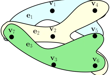
The basic idea of our solution approach is to turn the problem into a flow control one. To do this, consider the hypergraphH with vertex set V and edgeset E as:
H :={V,E}, V ={v1,...,vm}, E :={e1,...,en}.
The vertex set V has one vertex per each coalition whereas the edge set E has one edge per each player.
v
1
v
2
v
3
v
4
v
5
v
6
v
7
e
1
e
3
[image:2.612.323.552.465.620.2]e
2
Fig. 1. HypergraphH:={V,E}for a 3-player coalitional game.
A generic edge i is incident to a vertex vj if the player i
is in the coalition associated to vj. So, incidence relations are
described by matrix BH = [cT
S]S⊆N ∈Rm×n whose rows are
the characteristic vectors of all coalitions S⊆N.
vS(t) of a generic coalition S as the demand dj(t) in the corresponding vertex vj, namely vS(t) =dj(t). At this point
we can introduce a dnom andΔd(t)so that, in the future, we
can again use the expression d(t) =dnom+Δd(t) in analogy
with v(t) =vnom+Δv(t).
In view of this, allocation in the core translates into satis-fying in excess the demand at the vertices. Specifically,
˜
a(t)∈C(v˜(t)) ⇔ BHa˜(t)≥d˜(t) (1) Now, since ˜d(t) is unknown at time t, we need to introduce some error dynamics which accounts for the derivatives of excesses:
˙
ε(t) =BHa(t)−d(t), d(t)∈V.
With the above in mind, the problem can be turned into a flow control problem where a controller wishes to drive the error
ε(t)(the excesses) to a target set
T :={ε∈Rm:εm=0,εj≥0,∀j=1,...,m−1}.
But we can do more than this to simplify the tractability of
1
2
m
(0)
[image:3.612.321.553.202.310.2](
t
)
Fig. 2. Trajectory forε(t).
the problem. Using standard LP techniques we can introduce m−1 surplus variables (one per each coalition other than the grand coalition) so to project the allocation space into a one of higher dimension. In particular, let us expand control u(t) =
[a(t)T s(t)T]T ∈R(n+m−1). This technique has the advantage of turning the inequalities (1) into equalities of type (see, e.g., [4], [5]):
˙
x(t) =Bu(t)−d(t), d(t)∈V,
where matrix B is defined as
B=
BH −I
0
∈Rm×(n+m−1)
and I is an identity matrix of compatible dimensions. Variable x(t)∈Rmis now the state of the system. In order to rephrase
the original problem in terms of a flow control problem, we still have to introduce the feasible controls set
U :={u∈Rn+m−1: a∈A,s≥0} ∈Rn+m−1 (2)
and define a new vector unom= [aTnom sTnom]T ∈U satisfying
Bunom=vnom.
We hereafter abbreviate “with probability one” and write “w.p.1”.
We are now ready to restate the original problem as follows. Find a control strategyφ:Rm→U which drives the state x(t) to zero in probability and returns the desired average control unom:
u(t):=φ(x(t))∈U⇔lim
t→∞x(t) =0 w.p.1, and limt→∞u(t) =unom.
Stating differently, we require the dynamics ˙x(t) =Bφ(x(t))− d(t)to be stochastically stable withφ(x(t))satisfying certain average constraints.
˙
x(t) =BΔu(t)−Δd(t)
z(t) =B† F
⎡ ⎣x(t)
y(t)
⎤ ⎦
ˆ
φ(z(t))
u(t)
d(t)
˙
y(t) =CΔu(t)
Fig. 3. Dynamical system.
IV. STOCHASTIC STABILITY AND AVERAGE CONSTRAINTS In this section, we state the main result of this work which proposes a solution to Problem 1. Before stating the result we need to modify the dynamics (8) in the way explained next. First denote by B† a generic pseudo inverse matrix of B and complete matrices B and B†with matrices C and F such that
B
C B
† F =I. (3)
Then, building upon the new square matrix
B C
, let us move
to consider the augmented system
˙
x(t) = BΔu(t)−Δd(t) ˙
y(t) = CΔu(t). (4)
After integrating the above system (see (5), right) we come up with a new variable z(t)(see (5), left), that plays a central role for the problem at hand:
z(t) = B† F x(t) y(t)
,
x(t) y(t)
=
B C
z(t). (5)
Indeed, it turns out that to drive x(t) to zero w.p.1, and obtain unom as average allocation on the long run, we can
rely on a simple function ˆφ(.), which depends on z(t). Before introducing this function, for future purposes observe that the dynamics for z(t)satisfies the first-order differential equation:
˙z(t) = B† F x˙(t) ˙ y(t)
= B† F B
C
Δu(t)− B† F Δd(t) 0
= Δu(t)−B†Δd(t).
[image:3.612.90.262.309.465.2]Back to the function ˆφ(z(t)), let Δumin and Δumax be the minimal and maximal values of Δu(t) for the following constraints to hold true: u(t) =unom+Δu(t)∈U . Then, let us
formally define ˆφ(z(t))as: ˆ
φ(z(t)):=unom+Δu(t)∈U, Δu(t) =sat[Δumin,Δumax](−z(t)),
(7) where with sat[a,b](ξ) we denote the saturated function that, given a generic vector ξ and lower and upper bounds a and b of same dimensions asξ, returns
sat[a,b](ξ)=.
⎧ ⎨ ⎩
bi for all i ξi>bi
ai for all i ξi<ai
ξi for all i ai≤ξi≤bi
.
Now, taking the control u(t) = φˆ(z(t)), we obtain the dynamic system ˙x(t) =B ˆφ(z(t))−d(t) as displayed in Fig. 3. With the above preamble in mind, we are ready to state the following convergence property.
Theorem IV.1 The dynamic system (8) with ˆφ(z(t))as in (7) converges to zero w.p.1 and satisfies limt→∞u¯(t) =unom:
˙
x(t) =B ˆφ(z(t))−d(t). (8) Proof: Consider a candidate Lyapunov function V(z(t)) = 1
2z
T(t)z(t). The idea is to inspect that E[V˙(z(t))]<0 for all
t≥0. To see that this last is true, observe that from (6) we have
E[V˙(z(t))] = E[zT(t)˙z(t)]
= E[zT(t)Δu(t)]−E[zT(t)B†Δd(t)]
= E[zT(t)sat(−z(t))]<0,
where condition E[zT(t)B†Δd(t)] =0 is a direct consequence of Assumption 4 which translates into Δd(t) being uncor-related with zT(t). But the above condition implies that limt→∞z(t) =0 w.p.1, which, from (5)-left, and[B†F] being
non singular and square, leads to limt→∞x(t) =0 w.p.1 as
well.So far we have proved the first part of the statement, i.e., that the dynamic system (8) converges to zero w.p.1. For the second part, after integrating dynamics (6), we have
lim
t→∞
t
0[Δu(τ)−B†Δd(τ)]dτ t =tlim→∞
z(t)−z(0) t =0. This last condition together with the assumption vnom :=
limt→∞v¯(t)yield
lim
t→∞
t
0B†Δd(τ)dτ t =tlim→∞
t
0Δu(τ)dτ
t =0
from which we can conclude limt→∞u¯(t) =
limt→∞ t
0unom+Δu(τ)dτ
t =unom as claimed in the statement.
In the next corollary, we use the previous result to provide an answer to Problem 1.
Corollary IV.1 The average allocation converges to the nom-inal allocation:
lim
t→∞a¯(t) =anom.
Proof: This is a direct consequence of the result proved in the previous theorem: limt→∞u¯(t) =unom.
V. NUMERICAL ILLUSTRATIONS
Consider a 3 player coalitional TU game, so m=7, with the following intervals for values of coalitions:
v({1})∈[0,4], v({2})∈[0,4], v({3})∈[0,4], v({1,2})∈[0,4], v({1,3})∈[0,6],
v({2,3})∈[0,7], v({1,2,3})∈[0,12].
The convex set V is then a hyperbox characterized by the above intervals. >From Assumption 4, the GD knows the long run average game, i.e., limt→∞v¯(t) =vnom. Without loss of
generality we take the balanced nominal game be as vnom= [1 2 3 4 5 6 10]T. In other words, during the simulations we randomize the instantaneous games v(t)∈V so that it satisfies the average behavior given by:
lim
t→∞
1 t
t
0
v(τ)dτ=vnom. (9)
Next, we describe an algorithm to generate v(t)∈V such that the above condition holds true.
Algorithm:
1) Generate m random points, ri∈V ⊂Rm, i=1,2,···,m.
2) Solve R.p=vnom, with R= [r1, r2,··· rm].
3) If p≥0 and 1Tp>0, then go to (4) else go to (1).
4) Rescale R as R=1TpR and p as p= p (1Tp)
5) If ri∈V, i=1,2,···,m, then go to (6) else go to (1).
6) STOP
By construction of the algorithm, vnomis in the relative interior
of the convex hull generated by the columns of the matrix R. If an instance of the game v(t)is chosen as riwith probability pi
from the pair(R,p), Assumption 4 is satisfied. For simulations we ran the algorithm 20 times to generate a total of 140 points (or 20(R,p)pairs) inV. Further, from each of the 20 pairs we take 2000 random selections (using Matlabrandsrc
function), which amounts to 40,000 instantaneous games v(t). The nominal choice of allocations and surplus is taken as unom= [2.5 3 4.5 1.5 1 1.5 1.5 2 1.5]T. It can be verified that Bunom=vnom.
For simulations, the saturation thresholdsΔumin andΔumax are chosen so as to ensure u(t)∈U . This condition translates into Umin≤unom+sat[Δumin,Δumax]≤Umax. Denote 1 as a vector with all entries equal to 1. For the instantaneous game a negative allocation/surplus is not allowed, so Umin ≥0·1.
Further, an allocation/surplus greater than the value of grand coalition is not allowed, so Umax≤vnom(N)·1. For the given
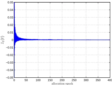
game parameters, we see that the lower and upper thresholds for the saturation function are −1 and 5.5 respectively. The robust allocation rule is implemented numerically with a step size of Δ =0.01. Next, we present some significant performance results of the robust control law given by equation (7). >From Theorem IV.1, limt→∞¯z(t)converges to zero with
0 50 100 150 200 250 300 350 400 −0.05
−0.04 −0.03 −0.02 −0.01 0 0.01 0.02 0.03 0.04 0.05
allocation epoch
¯
z1
(
t
[image:5.612.73.263.62.207.2])
Fig. 4. Performance of the robust control law ˆφ(z(t)): time plot of first component of ¯z(t).
4 illustrates this behavior for the first component of z(t). Further, by Corollary IV.1, the same control law ensures that the average game is balanced in the long run, in other words limt→∞x¯(t) =0. The control law ensures that E[V˙(z(t))] is
0 50 100 150 200 250 300 350 400 −0.5
−0.4 −0.3 −0.2 −0.1 0 0.1
allocation epoch
E
[˙
V
(
t
[image:5.612.347.526.64.210.2])]
Fig. 5. Time plot of E[V˙(x(t))]
negative for all t >0; we illustrate this behavior in Fig. 5. From Corollary IV.1, we also know that the average allocation vector converges to the nominal allocation vector. We illustrate this fact in Fig. 6. Here, we notice that convergence occurs with an approximation error of about 10−2. This reflects the fact that, in generating the instantaneous games v(t)through the above algorithm, the average value of B†Δd(t) converges to zero with, more or less, the same error as evident from looking at Fig. 7. We can interpret the average value ofΔd(t) as a measure of the uncertainty in learning the nominal game vnom, as given by (9). So, we believe an improvement in the
numerical precision while generating the instantaneous games v(t)will result in the exact convergence of the allocations.
VI. CONCLUSIONS AND FUTURE WORK
In this paper we derived a robust control law that ensures that the average allocation vector converges to the nominal
0 50 100 150 200 250 300 350 400 −0.05
−0.04 −0.03 −0.02 −0.01 0 0.01 0.02 0.03 0.04 0.05
allocation epoch ¯ a1(t)−anom(1)
¯ a2(t)−anom(2)
¯ a3(t)−anom(3)
Fig. 6. Time plot of ¯a(t)−anom.
0 50 100 150 200 250 300 350 400 −0.05
−0.04 −0.03 −0.02 −0.01 0 0.01 0.02 0.03 0.04 0.05
allocation epoch
B
†Δ
d2
(
t
[image:5.612.338.525.65.392.2])
Fig. 7. Time plot of second component of B†Δd(t).
allocation vector on the long run. However, the control law is derived on the premise that the GD knows apriori, the nominal allocation vector. If this information is not available the derivation of the control law implicitly involves solving an LP problem. By further relaxing the information requirement, the problem can be treated as a learning process where the GD is trying to learn the nominal game from the instantaneous games. We postpone working in this direction for the future.
REFERENCES
[1] S.Z. Alparslan Gök, S. Miquel, and S. Tijs, “Cooperation under interval uncertainty”, Mathematical Methods of Operations Research, vol. 69, no. 1, 2009, pp. 99–109.
[2] T. Arnold., U. Schwalbe, “Dynamic coalition formation and the core”,
Journal of Economic Behavior and Organization, vol. 49, 2002, pp.
363–380.
[3] D. Bauso and P. V. Reddy, “Robust allocation rules in dynamical cooperative TU Games”, accepted to the 49th IEEE Conf. on Decision
and Control, Atlanta, Georgia, USA, Dec 2010.
[4] D. Bauso and J. Timmer, “Robust Dynamic Cooperative Games”,
International Journal of Game Theory, vol. 38, no. 1, 2009, pp. 23–
36.
[5] D. Bauso, J. Timmer, “On robustness and dynamics in (un)balanced coalitional games”, Memorandum 1916, Department of Applied
Mathe-matics, University of Twente, 2010, ISSN 1874-4850.
[image:5.612.76.263.332.485.2][7] F. Blanchini, “Set invariance in control – a survey”, Automatica, vol 35, no. 11, pp. 1747–1768, 1999.
[8] J.C. Cesco, “A convergent transfer scheme to the core of a TU-game”,
Revista de Matemáticas Aplicadas, vol. 19, no. 1-2, 1998, pp. 23–35.
[9] J.A. Filar and L.A. Petrosjan, “Dynamic Cooperative Games”,
Interna-tional Game Theory Review vol. 2, no. 1, 2000, pp. 47–65.
[10] J. H. Grotte, “Dynamics of cooperative games”, International Journal
of Game Theory, vol. 5, no. 1, pp. 27–64.
[11] A. Haurie, “On some Properties of the Characteristic Function and the Core of a Multistage Game of Coalitions”, IEEE Transactions on
Automatic Control, vol. 20, no. 2, 1975, pp. 238–241.
[12] L. Kranich, A. Perea, H. Peters, “Core concepts in dynamic TU games”,
International Game Theory Review, vol. 7, 2005, pp. 43–61.
[13] E. Lehrer, “Allocation Processes in Cooperative Games”, International
Journal of Game Theory, vol. 31, 2002, pp. 341–351.
[14] A. Sengupta, K. Sengupta, “A property of the core”, Games and
Economic Behavior, vol. 12, 1996, pp. 266–273.
[15] J. Suijs and P. Borm, “Stochastic Cooperative Games: Superadditivity, Convexity, and Certainty Equivalents”, Games and Economic Behavior, vol. 27, no. 2, 1999, pp. 331–345.
[16] J. Timmer, P. Borm, and S. Tijs, “On three Shapley-like solutions for cooperative games with random payoffs”, International Journal of Game