‘Quantum’ Parallel computation with neural networks

(1)

Department of Computer Science, University of York

Submitted in part fulfilment for the degree of MEng

Nathan Burles

10 May 2010

Word count: 23,989 on 70 pages as counted by the Microsoft Word word count command. This includes the glossary, but excludes all appendices.

‘Quantum’ Parallel computation

(2)

(3)

Abstract

Correlation matrix memories have been successfully applied to many domains. This work implements a production system put forward in [Austin, 2003], to demonstrate its viability as an efficient rule-chaining process. Background information on rule-chaining and CMMs is given, followed by a review of the proposed production system.

Throughout the iterative development process, experimentation is performed in order to investigate the effects of changing the properties of vectors used in this system. The results show that generating vectors using the algorithm proposed in [Baum, 1988] with a weight close to log2 of the vector length provides the highest storage capacity.

The simple system implemented in this work performs rule-chaining effectively. This leads to the conclusion that the proposed production system is viable, and that this area warrants further work.

Acknowledgements

(4)

List of figures

Figure 1: Finite state machines ... 9

Figure 2: Qubit in superposition of states ... 12

Figure 3: Computational basis set ... 12

Figure 4: Equal superposition basis set ... 12

Figure 5: Qubit in unknown state ... 12

Figure 6: Feed-forward artificial neural network ... 14

Figure 7: Common neuron functions ... 14

Figure 8: Neural network for back propagation ... 15

Figure 9: A binary correlation matrix memory ... 16

Figure 10: Training a binary correlation matrix memory ... 17

Figure 11: Recalling a pattern from a binary correlation matrix memory ... 17

Figure 12: Two-layer correlation matrix memory ... 21

Figure 13: Example rule set ... 22

Figure 14: Example rule set without disjunctions ... 23

Figure 15: Correlation matrix memory trained with example rule set ... 24

Figure 16: Tensor product of token Z with state S0 ... 25

Figure 17: Superposition of tensor products ... 25

Figure 18: Simple two-layer CMM ... 26

Figure 19: Two-layer example rule set ... 26

Figure 20: Recall of a tensor product ... 27

Figure 21: Undistinguishable recall of superimposed states ... 27

Figure 22: Two-layer example rule set with tensor products ... 28

Figure 23: Correct recall of superimposed states ... 28

Figure 24: Complete two-layer CMM rule-chaining system (adapted from [1]) ... 29

Figure 25: Example rule set for arity networks ... 30

Figure 26: Arity networks ... 30

Figure 27: Probability of recall error ... 35

Figure 28: Number of vector pairs recalled against vector weight... 35

Figure 29: Number of vector pairs recalled against vector weight, with updated code ... 40

Figure 30: Rule set used in testing rule-chaining ... 42

Figure 31: Identifying tensors within a tensor product ... 45

Figure 32: Identifying vectors within a tensor product ... 45

Figure 33: Probability of recall error from a tensor product ... 49

Figure 34: Number of tensor products successfully recalled for a given tensor length ... 50

Figure 35: Probability of recall error from a tensor product using tensor detection algorithm ... 51

Figure 36: Two methods to recall a tensor product ... 53

Figure 37: Tensor product training and recall ... 54

Figure 38: Recall using a two-layer CMM network ... 55

Figure 39: Memory requirements of a CMM using a sparse matrix ... 58

Figure 40: Number of additional bits set in the output of a system trained with 200 rules ... 59

(7)

List of equations

Equation 1: Input to a neuron ... 14

Equation 2: Sigmoidal function ... 14

Equation 3: n choose k ... 19

Equation 4: Maximising n choose k ... 19

Equation 5: Probability of recall failure ... 20

Equation 6: Bits required in a one-layer CMM ... 21

Equation 7: Bits required in a two-layer CMM ... 21

List of tables

Table 1: Willshaw thresholding ... 18

Table 2: L-max thresholding ... 18

Table 3: Vectors generated using Baum’s algorithm ... 18

Table 4: L-wta thresholding ... 18

Table 5: Probability of recall error given a vector length of 10 ... 20

Table 6: Rule set with assigned vectors ... 23

Table 7: Tree search performed on the example ... 24

Table 8: State tokens with assigned vectors ... 25

Table 9: Lengths and weights to allocate a given number of vectors ... 26

Table 10: Probability of recall error ... 34

Table 11: Probability of recall error using tensor product recall ... 39

Table 12: Probability of recall error, with updated code ... 39

Table 13: Results of testing rule-chaining ... 43

Table 14: Possible tensors within a tensor product ... 45

Table 15: Generation of lexicographic and Baum vectors ... 46

Table 16: Number of tensor products successfully recalled for a given tensor weight ... 49

Table 17: Unique tensors that may be generated for a given length and weight ... 52

Table 18: Memory requirements without a sparse matrix representation ... 58

Table 19: Number of tensor products superimposed against number of rules trained ... 60

(8)

1 Introduction

Artificial neural networks were designed as an attempt to mimic the higher functions of the animal brain, particularly for applications such as pattern recognition. Correlation matrix memories (CMMs) are a special class of neural network that have the benefit of a fast, online training algorithm.

CMMs have been successfully applied to many and varied domains, including pattern recognition [35], chemical similarity searching [26], and spell checking algorithms [22]. This work is concerned with the application of rule-chaining, or inference.

1.1 Aims

The main aim of this work is to show whether the rule-chaining system proposed in [1] is a feasible application of CMMs. A simple CMM is required in order to demonstrate this, as well as a classical system in which to store rules for comparison.

Experimentation will be performed at each stage of the development of the final system. This is in order to fulfil the secondary aims of this work, namely to investigate the properties of CMMs, vectors, and tensor products.

1.2 Report structure

Chapter 2 introduces the background information to this work, progressing gradually through the field of knowledge. This chapter initially gives a basic description of finite state architectures, before introducing rule-chaining. A very limited introduction to quantum computation follows, in order to demonstrate the benefits that may be achieved through the use of superposition. Next is a description of neural networks, with CMMs in the following section. Finally, a detailed explanation of the proposed method of rule-chaining is given.

The following six chapters describe the development and experimentation performed within this work. Chapter 3 contains the initial planning that is imperative when performing an iterative development. Each of the remaining development chapters contain a series of sections that match the stages of the iterative development process: overview, design, implementation, testing, results, and evaluation. Chapter 4 describes the first iteration, which is the development of a simple CMM. Chapter 5 moves on to investigate the use of tensor products that can later allow the superposition of tokens, and Chapter 6 extends this by performing rule-chaining – taking the output of a CMM directly back to be an input. Chapter 7 explores the superposition of tensor products, and Chapter 8 examines the final system of this work.

Finally, Chapter 9 gives the conclusions made within this work, as well as making some further conclusions. Some possible future work is also described, such as the implementation of arity networks, and the mathematical proof of improvements that the CMM system can offer in comparison to a classical system with regards to time or space complexity.

1.3 Statement of ethics

(9)

2 Literature review

This chapter presents the background information to this work, gradually focusing on the techniques used to perform rule-chaining within a CMM network. Section 2.1 gives a brief introduction to finite state architectures, and Section 2.2 builds upon this with a description of rule-chaining. Section 2.3 is a simple description of quantum computation and the benefits that superposition can offer. Section 2.4 introduces neural networks, while Section 2.5 describes a particular class of neural networks known as a CMM. Finally, Section 2.6 details the techniques that have been proposed to perform rule-chaining using CMMs.

2.1 Finite state architectures

Finite state architectures can be used to model the behaviour of a system, or object within a system [11]. They can be represented as a 5-tuple M = (Q, Σ, q0, δ, A) [31], where:

• Q is a finite set of states

• _{Σ is an alphabet of input symbols} • q0 ∈ Q is the initial state

• _𝛿𝛿:Q × Σ → Q is the transition function • A ⊆ Q is the set of accepting states

a: Finite state acceptor b: Moore machine c: Mealy machine Figure 1: Finite state machines

More simply, they can be thought of as a directed graph (Figure 1), with three main elements: • A finite set of states, represented as nodes

• State transitions, represented as edges

• Input symbols, governing which state transition should be taken given the current state Finite state machines (FSM) are often categorised into two classes – acceptors and transducers [30]. A finite state acceptor (FSA) is an automaton that will simply accept or reject an input string, and as such they can be used to recognise a language. This class of automaton (Figure 1a) is most widely described in literature as it is simple, yet powerful, and can be used for purposes such as lexical analysis.

(10)

A Moore machine produces output in each state [32]. In contrast to this, Mealy machines produce output in each transition [33]. Although the two types of FST differ in how they represent and produce an output, they actually have the same expressive power as “it is possible to convert any Mealy type machine into an equivalent Moore type machine, and vice-versa” [18].

2.2 Rule-chaining

Logic is the study of reasoning – forming conclusions from a set of premises [17]. These arguments are commonly given in the form:

𝑃𝑃𝑃𝑃𝑃𝑃𝑃𝑃𝑃𝑃𝑃𝑃𝑃𝑃 1 𝑃𝑃𝑃𝑃𝑃𝑃𝑃𝑃𝑃𝑃𝑃𝑃𝑃𝑃 2 𝐶𝐶𝐶𝐶𝐶𝐶𝐶𝐶𝐶𝐶𝐶𝐶𝑃𝑃𝑃𝑃𝐶𝐶𝐶𝐶

Alternatively, it can be more efficient to use an inline form of propositional logic, for example: 𝑃𝑃𝑃𝑃𝑃𝑃𝑃𝑃𝑃𝑃𝑃𝑃𝑃𝑃 1∧ 𝑃𝑃𝑃𝑃𝑃𝑃𝑃𝑃𝑃𝑃𝑃𝑃𝑃𝑃 2⇒ 𝐶𝐶𝐶𝐶𝐶𝐶𝐶𝐶𝐶𝐶𝐶𝐶𝑃𝑃𝑃𝑃𝐶𝐶𝐶𝐶

In this report, I will use the inline representation and a subset of the syntax used in [38], specifically: ¬_{𝑝𝑝 𝑁𝑁𝑃𝑃𝑒𝑒𝑒𝑒𝑒𝑒𝑃𝑃𝐶𝐶𝐶𝐶 − 𝐶𝐶𝐶𝐶𝑒𝑒 𝑝𝑝}

𝑝𝑝 ∧ 𝑞𝑞 𝐶𝐶𝐶𝐶𝐶𝐶𝐶𝐶𝐶𝐶𝐶𝐶𝐶𝐶𝑒𝑒𝑃𝑃𝐶𝐶𝐶𝐶 − 𝑝𝑝 𝑒𝑒𝐶𝐶𝑎𝑎 𝑞𝑞 𝑝𝑝 ∨ 𝑞𝑞 𝐷𝐷𝑃𝑃𝑃𝑃𝐶𝐶𝐶𝐶𝐶𝐶𝐶𝐶𝑒𝑒𝑃𝑃𝐶𝐶𝐶𝐶 − 𝑝𝑝 𝐶𝐶𝑃𝑃 𝑞𝑞

𝑝𝑝 → 𝑞𝑞 𝐼𝐼𝑃𝑃𝑝𝑝𝐶𝐶𝑃𝑃𝐶𝐶𝑒𝑒𝑒𝑒𝑃𝑃𝐶𝐶𝐶𝐶 − 𝑝𝑝 (𝑒𝑒ℎ𝑃𝑃 𝑒𝑒𝐶𝐶𝑒𝑒𝑃𝑃𝐶𝐶𝑃𝑃𝑎𝑎𝑃𝑃𝐶𝐶𝑒𝑒) 𝑃𝑃𝑃𝑃𝑝𝑝𝐶𝐶𝑃𝑃𝑃𝑃𝑃𝑃 𝑞𝑞 (𝑒𝑒ℎ𝑃𝑃 𝐶𝐶𝐶𝐶𝐶𝐶𝑃𝑃𝑃𝑃𝑞𝑞𝐶𝐶𝑃𝑃𝐶𝐶𝑒𝑒)

There are two methods of inference commonly used for rule-chaining – forward chaining and backward chaining [40]. In propositional logic, both of these types of reasoning have the same goal. They approach the problem of forming a conclusion from a series of premises from opposing angles. 2.2.1 Inference

Forward chaining, also known as data-driven rule-chaining [13], searches the available rules in order to find one for which the antecedent is known to be true. This allows the current state to be updated to include the consequent of that rule. By repeated application of this process, the goal may be achieved. This process effectively implements a finite state machine, although commonly with few or no cycles.

The alternative, backward chaining, can be known as goal-driven rule-chaining [13]. In this method, all rules with a consequent matching the desired goal and with antecedents that are not known to be false are added to the current state. This is repeated, with new rules added such that their consequents match the antecedents already in the current state, until a rule is found that has an antecedent that is known to be true.

To better explain the mechanisms used by forward and backward chaining, I have adapted an example from [13]. The goal is to determine the mood of a university professor, given that they are currently lecturing, and the knowledge held by the system is:

(11)

Using forward chaining, the antecedents of all the rules are checked against the current state. Rule 1 matches, and so the consequent 𝐶𝐶𝑜𝑜𝑃𝑃𝑃𝑃𝑜𝑜𝐶𝐶𝑃𝑃𝑜𝑜𝑃𝑃𝑎𝑎 is added to the state. The knowledge base is searched again, and this time rule 3 matches, resulting in 𝑒𝑒𝑃𝑃𝐶𝐶𝑃𝑃𝑝𝑝𝑔𝑔 being added to the state. At this point the system may perform one of two actions:

1. Halt, if it has further information that enables it to recognise 𝑒𝑒𝑃𝑃𝐶𝐶𝑃𝑃𝑝𝑝𝑔𝑔 as a possible mood, and hence conclude that it has reached the goal.

2. Perform a further search of the knowledge base to determine if there are any further rules whose antecedents match. If there are not, then it may conclude that the final state reached was the goal state.

In backward chaining, the consequents of all the rules are checked against the goal state – and so the system is required to hold further information as to what constitutes a “mood”. Rules 3 and 4 both match the goal, and so their antecedents are compared to the current state to check for consistency. Neither 𝐶𝐶𝑜𝑜𝑃𝑃𝑃𝑃𝑜𝑜𝐶𝐶𝑃𝑃𝑜𝑜𝑃𝑃𝑎𝑎 nor 𝑃𝑃𝑃𝑃𝑃𝑃𝑃𝑃𝑒𝑒𝑃𝑃𝐶𝐶ℎ𝑃𝑃𝐶𝐶𝑒𝑒 are currently known to be either true or false, and so both of these antecedents are added to the goal list. The knowledge base is searched again, and this time rules 1 and 2 match the goals. Upon checking their antecedents, the system is able to eliminate rule 2, and confirm rule 1. This confirmation leads to the proof of rule 3, which in turn gives the desired goal.

It is claimed that “forward checking is another ... technique which offers an improvement over the inefficient behaviour of chronological backtracking” [40]. On the other hand, [13] argues that “whether you use forward or backwards reasoning to solve a problem depends on the properties of your rule set and initial facts”. In general, forward chaining has been found to be more efficient than backward chaining for applications such as agent control in the context of artificial intelligence [38], or a tree-based database search [13]. Complementary to this backward chaining is well suited to applications such as proving a fact, given a particular knowledge base – for example Prolog uses this technique when performing Selective Linear Definite (SLD) clause resolution [17].

2.3 Quantum computation

It is stated that:

Quantum computation and quantum information is the study of the information processing tasks that can be accomplished using quantum mechanical systems. [34]

The motivations and mechanics behind quantum computation are outside the scope of this work; however some of the concepts are important to understand. The most important of these concepts is superposition, and the reduction in computational complexity that can be achieved as a result of its use.

(12)

Bra-ket, or Dirac, notation is commonly used to represent the state of a qubit |𝜓𝜓⟩ and whereas a classical bit may be in one of two states – often represented as 0 or 1 – a qubit may be in a superposition of states [34]:

|𝜓𝜓⟩=𝛼𝛼|0⟩+𝛽𝛽|1⟩ _{superposition of states}Figure 2: Qubit in

where 𝛼𝛼 and 𝛽𝛽 are complex numbers. 2.3.1 Basis sets

A basis set can be described as a minimal set of orthonormal states such that any other state may be described as a linear combination of those states [10]. The simplest set of basis states for a single qubit is known as the computational basis set. This comprises of:

|0⟩= 1|0⟩+ 0|1⟩

|1⟩= 0|0⟩+ 1|1⟩ Figure 3: Computational basis set

The computational basis set is useful for representation of states, however in order to exploit the potential parallelism that quantum computation offers, a basis set comprising of an equal superposition of states is commonly used. Represented in the computational basis, for a single qubit system these states are:

|+⟩= 1

√2|0⟩+ 1 √2|1⟩

|−⟩= 1

√2|0⟩ − 1 √2|1⟩

Figure 4: Equal superposition basis set

2.3.2 Measurement collapses an unknown state

Although a qubit may be in one of infinitely many combinations of states, it is not possible to determine what that state is through measurement [34]. That is to say, for a qubit in state:

|𝜓𝜓⟩=𝛼𝛼|0⟩+𝛽𝛽|1⟩ Figure 5: Qubit in unknown state

the coefficients 𝛼𝛼 and 𝛽𝛽 denote the probability of finding a particular state upon measurement. The result will either be a 0 with a probability of |𝛼𝛼|2_{or a 1 with a probability of |𝛽𝛽|}2_{, where the sum of} the probabilities is 1.

In addition to this limit, the action of performing a measurement on a qubit changes the state – causing it to collapse from an unknown superposition of |0⟩ and |1⟩ to one of the computational basis states, equal to the result of the measurement [34].

2.3.3 Grover’s algorithm

(13)

Instead of this, the advantage of quantum computing is the ability to solve problems that are infeasible using a classical computer [34], and the challenge is in designing algorithms and quantum circuits to do so. Examples of this, that offer very impressive results, include Shor’s algorithm [41] and Deutsch’s algorithm [15].

Grover’s algorithm [19] is most relevant to this work, however, as it is an algorithm capable of improving the computational complexity of a database search.

Explained by Nielsen:

Given a search space of size N, and no prior knowledge about the structure of the information in it, we want to find an element of that search space satisfying a known property. [34]

In a classical system, and in the worst case, this search will require 𝑁𝑁 operations in order to obtain a result. Grover’s algorithm is capable of obtaining a result in only √𝑁𝑁 operations; a quadratic improvement. This is a smaller improvement than found in the previously mentioned algorithms; however it is still a significant gain, especially when the database is very large.

This section on quantum computation is only written as a simple introduction to the field, as there are many sources from which a more detailed explanation can be obtained (such as [10], [25], and [34]). It is, however, intended to highlight the potential improvement that can be achieved by computing using a superposition of states as opposed to the brute-force approach which must be applied to many of these problems when using conventional computation.

2.4 Neural networks

Traditional – or hard – computing is concerned with the precision and certainty of a solution, and rigour in the approach to obtaining that solution [49]. Soft computing, on the other hand, is “tolerant of imprecision, uncertainty, partial truth, and approximation” [24]. Within soft computing are three main fields: fuzzy logic, neural networks, and probabilistic reasoning [49].

Neural networks are “a biologically inspired approach to the pattern recognition problem” [48]. The animal brain consists of a great number of neurons, each connected to many other neurons by synapses. Artificial neural networks were designed to simulate this behaviour, as an attempt to reproduce our natural ability at pattern recognition. As each neuron within a network is fully self-contained, the system can be designed to be massively parallel [48]. It is important to emphasise that although neural networks are inspired by biological processes, they need not be constrained by them: the accurate modelling of biological neural networks, and the processes within them, is a field in its own right [47].

2.4.1 Feed-forward neural networks

(14)

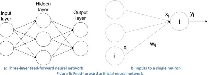
a: Three-layer feed-forward neural network b: Inputs to a single neuron Figure 6: Feed-forward artificial neural network

The output of a neuron is generated by applying a particular function to the weighted sum of its inputs. Figure 6b shows the inputs to a single neuron 𝐶𝐶, and the total input is given by [48]:

𝑥𝑥𝐶𝐶 =𝛼𝛼𝐶𝐶 +� 𝑜𝑜𝑃𝑃𝐶𝐶𝑥𝑥𝑃𝑃 𝑃𝑃→𝐶𝐶

Equation 1: Input to a neuron

where 𝑥𝑥𝑃𝑃 is the output of neuron 𝑃𝑃, 𝑜𝑜𝑃𝑃𝐶𝐶 is the weight of the connection from neuron 𝑃𝑃 to neuron 𝐶𝐶,

and 𝛼𝛼𝐶𝐶 is a constant offset, or bias.

The output 𝑔𝑔𝐶𝐶 of a neuron can then be calculated by applying a function to the value of the input 𝑥𝑥𝐶𝐶.

This function may be different for each neuron, as they are self-contained processing units, however it is common for the same function to be used for all neurons in a layer [47]. Although any function may be used, there are four that are most commonly found in artificial neural networks [39]:

a: Linear function b: Threshold function c: Linear threshold function d: Sigmoidal function

The threshold function (Figure 7b) effectively outputs a Boolean value, and as such is useful in the output layer of a neural network in order to generate a binary result [47]. The sigmoidal function (Figure 7d), on the other hand, most closely approximates the function used by biological neurons [39]. It is often used in the hidden layer in order that the neural network is able to represent non-linear relationships. The equation of this function is:

𝑔𝑔=_{1 +}1_𝑃𝑃_{−𝛼𝛼𝑥𝑥} Equation 2: Sigmoidal function where the value of 𝛼𝛼 controls the shape of the curve. In the limit 𝛼𝛼 → ∞, the sigmoidal function converges to become a threshold function [37].

[image:14.595.93.520.71.225.2]

(15)

by each neuron, the weights of each connection, or the number and position of neurons and connections. Generally, within the literature, most emphasis has been placed on the consequences of modifying the weights of connections between individual neurons as this is most likely to mimic the approach used in nature [36].

2.4.2 Back-propagation

[image:15.595.193.398.295.428.2]

There are various algorithms used to train neural networks, classified into one of two categories: supervised learning and unsupervised learning [42]. Supervised learning requires pairs of known inputs and outputs, a training set. The inputs are presented to the neural network, and the output generated in each case is compared to the desired output in order to generate information on the errors. The neural network is then able to apply an algorithm to update the connection weights in order to minimise these errors. This is in contrast to unsupervised learning, where only the inputs are provided and the neural network must update the connection weights in order to minimise a given function [42].

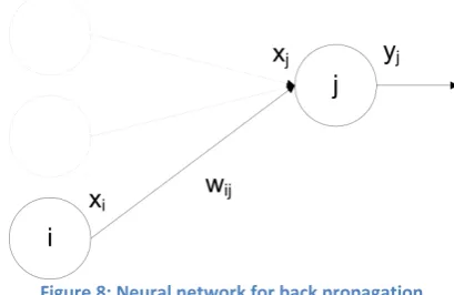
Figure 8: Neural network for back propagation

Due to its simplicity, one of the most common algorithms used within supervised learning is back-propagation [42]. A very limited description of this algorithm, restricted to only those neurons shown in Figure 8 can be described in 5 steps:

1. Present the neural network with an input taken from the training set.

2. Compare the output of neuron 𝐶𝐶 with that position of the desired output from the training set, and calculate the error value for this neuron.

3. Adjust the weights of each input connection to neuron 𝐶𝐶 in order to reduce the error.

4. Assign an error value to each of the neurons that input to neuron 𝐶𝐶. This is calculated as a portion of the error value of neuron 𝐶𝐶, and allocates more error to those connections with the highest weight as it considers those to be most to blame for the error.

5. Repeat from step 3 for neuron 𝑃𝑃, using the sum of all error values assigned to it from the neurons in the output layer.

(16)

are applied. They are particularly well suited to the problem of pattern recognition as that was one of the driving factors behind their development, and they are modelled loosely on the structure of the brain which is very effective at pattern recognition [39]. However, neural networks have been used for a wide range of applications including control, database retrieval, and fault-tolerant computing [42].

2.5 Correlation matrix memories

A particular class of neural networks is often known as a RAM-based neural network. These include multi-layered weighted networks, such as the Probabilistic Logic Node (PLN) amongst others. In addition to this, however, are also single layer neural networks using only binary weights, such as the Multi-RAM Discriminator (MRD), or Advanced Distributed Associative Memory (ADAM) [2]. One of the subclasses of RAM based neural networks is called a CMM, of which ADAM is a particular implementation [5]. A CMM is “a simple binary associative neural network” [1] that utilises Hebbian learning to allow for high speed, online training.

Hebb wrote:

When an axon of cell A is near enough to excite a cell B and repeatedly or persistently takes part in firing it, some growth process or metabolic change takes place in one or both cells such that A’s efficiency, as one of the cells firing B, is increased. [20]

This refers to the work that Hebb had carried out to investigate how neurons within the human brain contribute to higher functions such as learning. Although ‘The Organization of Behavior’ was first published in 1949, this is still considered to be a valid theory for the human learning process, and was important in the initial development of artificial neural networks.

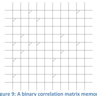
[image:16.595.220.376.455.609.2]

Figure 9: A binary correlation matrix memory

(17)

[image:17.595.74.524.361.537.2]

a: Present input and output vectors b: Store correlations Figure 10: Training a binary correlation matrix memory

2.5.1 Training

Training of a binary CMM requires only a single step, as shown in Figure 10. When the neural network is presented with an input and output vector (Figure 10a), any correlation between the two vectors is set in the matrix. That is to say, a neuron at the intersection of any horizontal wire that is set on the input with a vertical wire set on the output is itself set (Figure 10b).

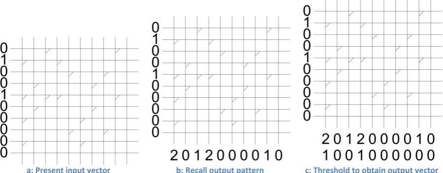
a: Present input vector b: Recall output pattern c: Threshold to obtain output vector Figure 11: Recalling a pattern from a binary correlation matrix memory

2.5.2 Recall

(18)

2.5.3 Thresholding

Deciding on a suitable threshold is the primary issue with regards to vector recall: there are various methods that may be used – Willshaw [7], L-max [3], and L-wta (Winner Takes All) [21] – each of which is suited to different applications [16].

3 1 2 1 0 a: Output pattern 1 1 1 1 0 b: Threshold at 1 1 0 1 0 0 c: Threshold at 2 1 0 0 0 0 d: Threshold at 3

Table 1: Willshaw thresholding

Using Willshaw thresholding, an absolute threshold value is selected: any integer in the output pattern that is greater than or equal to this threshold value is set in the output vector [46]. Selection of the threshold value is an important consideration, and will affect the retrieved vector as shown in Table 1. Various output vectors are shown, alongside the threshold value used to obtain them from the output pattern (Table 1a). In [45], Willshaw uses the weight of the input vector as the threshold value.

3 1 2 1 0 a: Output pattern 1 0 0 0 0 b: L=1

1 0 1 0 0 c: L=2 1 1 1 1 0 d: L=3

Table 2: L-max thresholding

L-max approaches the problem of thresholding from a very different angle. In this method, the L integers with the highest value in the output pattern are set in the output vector [12]. This is shown in Table 2, with various values for L; in circumstances when the output vector has a fixed weight, L can be selected to match this weight [21]. Table 2d is an example of a situation where the weight of the output vector differs from L – the algorithm is unable to distinguish the two integers with value 1 and so both are set in the output.

1 0 0 1 0 0 1 0 0 1 0 0 1 1 0 1 0 0 0 1 0 1 0 1 0 0 0 1 0 1

Table 3: Vectors generated using Baum’s algorithm

3 1 2 1 0 a: Output pattern 1 0 0 1 0 b: Sections {3,2} 1 0 1 0 0 c: Sections {2,3}

Table 4: L-wta thresholding

(19)

L-wta thresholding is essentially an extension of L-max that uses prior knowledge about the format of an output vector in order to improve recall accuracy. Each of the sections of an output pattern are thresholded individually, using L-max thresholding where L=1. Naturally, within each section, this suffers from the same problem as L-max thresholding, although the chance of this is reduced due to the segmentation of the vector. An example of L-wta thresholding is given in Table 4, using differing values for the lengths of each section in order to retrieve different output vectors.

It can be seen that all three of the thresholding methods has the potential to generate the same output vector, depending on the parameters used (Table 1c, Table 2c, and Table 4c). As such, the decision as to which method to use falls down to the application for which the CMM is to be used. Willshaw thresholding has the potential to be the fastest method available, due to the availability of an absolute threshold that need not be calculated in relation to the output pattern. On the other hand, for pattern recognition, L-max has been shown to be better at recalling vectors given an input that does not exactly match a trained pattern [7]. Finally, if the CMM is able to be trained using Baum generated vectors, then it was shown in [21] that there is a potential for up to 15% improvement in the capacity of the CMM by the use of L-wta.

2.5.4 Capacity

The allocation of vectors is a domain-specific problem, yet it greatly affects the potential capacity of a CMM. The number of fixed weight vectors that can be created by setting 𝑜𝑜 bits given a vector length 𝐶𝐶 is given by the equation for the binomial coefficient:

�𝐶𝐶𝑜𝑜�=_{𝑜𝑜! (𝐶𝐶 − 𝑜𝑜)!}𝐶𝐶! Equation 3: n choose k In the case of non-distributed vectors, where a vector has a weight of 1, this simply results in 𝐶𝐶 possible vectors. Using non-distributed vectors would mean that each bit within a vector represents an entire input or output pattern. This is infeasible for two reasons; due to inefficiency with regard to the storage capacity, but more importantly the lack of ability to generalise given a noisy input. A distributed representation is therefore typically used [4]. In order to maximise the number of possible vectors, 𝑜𝑜 can be chosen such that:

𝑜𝑜 ≅𝐶𝐶₂ Equation 4: Maximising n choose k

However, although this will allow the largest number of patterns to be represented by a fixed weight and fixed length vector, it does not necessarily follow that this will result in the highest capacity for a given CMM. As discussed by Austin and Stonham:

(20)

This is a probabilistic process, such that if the capacity of a CMM is surpassed, there is still a probability of correctly recalling each of the associated vectors. Given in terms of the probability of failure to perform a perfect recall:

𝑃𝑃= 1− �1− �1− �1−_{𝐻𝐻𝐻𝐻�}𝑁𝑁𝐼𝐼 𝑇𝑇�

𝐼𝐼

�

𝐻𝐻

Equation 5: Probability of recall failure

where 𝑃𝑃 is the probability of failure, 𝐻𝐻 and 𝐼𝐼 are the length and weight of the input vector respectively, 𝐻𝐻 and 𝑁𝑁 are the length and weight of the output vector respectively, and 𝑇𝑇 is the number of associated vectors. Equation 5 is derived fully in Appendix 1 of [7]. This equation is highly conservative, and a deeper analysis of the recall abilities within a CMM is given in [44] that returns a lower probability of error. This is unnecessary for the purposes of this review, however, where a pessimistic value will be sufficient.

Vector weight ₁ ₂ Number of vectors trained ₃ ₄ ₅

2 0.016 0.060 0.125 0.205 0.293

3 0.007 0.050 0.140 0.270 0.421

4 0.007 0.073 0.243 0.482 0.704

5 0.010 0.149 0.487 0.801 0.949

6 0.022 0.351 0.828 0.982 0.999

Table 5: Probability of recall error given a vector length of 10

It can be seen in Equation 5 that the probability of recall failure, and hence the potential capacity of a CMM, is directly affected by the ratio of length to weight for both input (𝐼𝐼/𝐻𝐻) and output (𝑁𝑁/𝐻𝐻) vectors. Table 5 contains values calculated for 𝑃𝑃, given that the input and output vectors have the same weight and a constant length of 10. With very few vectors trained, the probability of failure is smallest with a vector weight that is close to half of the vector length. It is clear, however, that as the vector weight increases, so does the rate of increase in 𝑃𝑃, given further trained vectors.

This is also the intuitive result: as the weight of the input or output increases, so more correlations will be stored in the CMM for every pair of input and output vectors that is trained. As the number of correlations stored in the CMM increases, so too does the probability that the presentation of a particular input will cause extra neurons to give an output. Initially this should not pose a problem, as the thresholding will be able to obtain the correct output vector with unexpected values in the output pattern. As the number of extra neurons that fire increases, however, so does the possibility that one of the values in the output pattern matches or even surpasses that of the correct output which will then threshold to give an incorrect output.

2.5.5 Pattern recognition using a two-layer correlation matrix memory

(21)

a: 1st correlation matrix memory b: 2nd correlation matrix memory Figure 12: Two-layer correlation matrix memory

It is shown in [7] that CMMs, as a specific class of neural network, also share this ability – in particular with regards to pattern recognition. Instead of simply associating two vectors directly in a single CMM, a two-layer associative memory is used (Figure 12). In the process that is described, the input vector is associated with an internally generated fixed-weight ‘class’ vector in the first CMM (Figure 12a). This class vector is then associated with the output vector within the second CMM (Figure 12b). A recall is performed in the same way as with a single-layer network, except that the thresholded output of the first CMM is then presented as an input to the second CMM.

In addition to the ability to recognise partially occluded patterns on an input, using a two-layer network has the potential to reduce the memory required in order to save the associations between large patterns [7]. In software implementations, such as that of the Advanced Uncertain Reasoning Architecture (AURA), a sparse matrix representation can be used in order to save only those values in the CMM that have been set [14]. In a hardware implementation, however, this is a lot more difficult and processing speed can be greatly reduced [43].

Assuming matrices are stored in their entirety, the number of bits required for a single-layer CMM to associate an input vector of length 𝐻𝐻 with an output vector of length 𝐻𝐻 would be:

𝑁𝑁𝐶𝐶𝑃𝑃𝑁𝑁𝑃𝑃𝑃𝑃 𝐶𝐶𝑜𝑜 𝑁𝑁𝑃𝑃𝑒𝑒𝑃𝑃 𝑃𝑃𝑃𝑃𝑞𝑞𝐶𝐶𝑃𝑃𝑃𝑃𝑃𝑃𝑎𝑎=𝐻𝐻𝐻𝐻 Equation 6: Bits required _{in a one-layer CMM}

In contrast, the number of bits required when using a two-layer network, where the internally generated vector has a length of 𝐶𝐶 is given by:

𝑁𝑁𝐶𝐶𝑃𝑃𝑁𝑁𝑃𝑃𝑃𝑃 𝐶𝐶𝑜𝑜 𝑁𝑁𝑃𝑃𝑒𝑒𝑃𝑃 𝑃𝑃𝑃𝑃𝑞𝑞𝐶𝐶𝑃𝑃𝑃𝑃𝑃𝑃𝑎𝑎=𝐻𝐻𝐶𝐶+𝐶𝐶𝐻𝐻 Equation 7: Bits required in a _{two-layer CMM}

Using a relatively small value for 𝐶𝐶, Equation 7 can give a far smaller memory requirement than Equation 6. If the value chosen is too small, however, it will limit the storage capacity of the neural network, and so this is a further consideration when designing a two-layer CMM for a particular task. 2.5.6 Applications and alternatives

(22)

This may serve to mask the potential applicability of these systems and techniques to a wide range of pattern matching problems. A few examples of the domains to which CMMs have been applied include chemical similarity searching [26], spell checking algorithms [22], and inference in expert systems [6]. These are essentially variations on a more general application of data mining within a knowledge base, with a domain-specific data representation and pre-processing and post-processing requirements.

A common alternative to using a CMM for these purposes would be to use a multi-layer neural network. This would provide the requisite pattern matching, and also generalise well to unknown or noisy inputs, however the major problem with this approach would be long training times [3]. Although [36] presents an online training algorithm for back-propagation, this only solves the requirement that all training of the neural network occurs prior to recall – training a new pattern is still a time-consuming process.

Using a CMM to search a knowledge base is also a lot more efficient than a conventional approach using a list, in terms of both time and space complexity [6]. CMMs are particularly well suited to searching unstructured data – a listing approach may be able to provide Ο(log𝐶𝐶) time complexity on structured data, but this degenerates to Ο(𝐶𝐶) with unstructured data. CMMs, on the other hand, are able to search any knowledge base with only a single pass through the network.

2.6 Rule-chaining in correlation matrix memories

Systems using propositional logic within neural networks have been designed and implemented with various underlying technologies (for example [9] and [28]). In addition, the theory regarding the use of CMMs in particular for propositional logic and inference has been developed in [6] and [29]. 2.6.1 Rule-chaining

As described in Section 2.2, rule-chaining is a method of inference also known as forward chaining. A system that performs forward chaining is often referred to as a production system. Using the pattern matching abilities of a CMM discussed in Section 2.5.5, rule-chaining in CMMs should be reasonably simple to implement. There are, however, a number of issues that must be resolved for the approach to be successful [1].

Rule-chaining is effectively a tree search, finding a path from an initial state to a goal. As such, anything described within this section may actually be adapted and applied to other problems involving a tree search.

As an illustration of rule-chaining, consider the rules in Figure 13 (adapted from [2]): 1. 𝑍𝑍 → 𝐵𝐵

(23)

Any rules that contain a disjunction in the antecedent are separated into multiple rules, as shown in Figure 14:

1. 𝑍𝑍 → 𝐵𝐵 2. 𝑍𝑍 → 𝐴𝐴 3. 𝐵𝐵 → 𝑋𝑋 4. 𝐵𝐵 → 𝑌𝑌 5. 𝐴𝐴 → 𝑌𝑌 6. 𝐴𝐴 → 𝑃𝑃 ∧ 𝑀𝑀

[image:23.595.234.359.613.723.2]

a: Set of rules b: Search tree, given an initial state of Z Figure 14: Example rule set without disjunctions

Each branch of the search tree is labelled (S1, S2, etc.) with what will be referred to as a state token. These represent the separation of paths within the tree – for instance there are two routes from 𝑍𝑍 to 𝑌𝑌, but they must remain independent during the search, especially if the aim of the search is to find the path to a goal rather than the goal itself.

2.6.2 Correlation matrix memories

When performing a tree search, there may be a large number of intermediate states to investigate between the initial state and the goal. In the most basic system, a search could be performed in various ways – the most common being depth-first and breadth-first. Both of these search methods have the disadvantage of a potential Ο(𝐶𝐶) time complexity.

In a conventional system, parallelism of a depth-first search could be used to improve this. At every branch, for instance, a new process could be created in order to continue the search along every possible path simultaneously. This would reduce the time complexity to Ο(𝑎𝑎), where 𝑎𝑎 is the maximum depth of the tree. Other problems would be posed, however, such as the requirement to maintain a large number of separate search processes. In addition to this, if the problem posed is one of finding the shortest route from the initial state to a particular goal state, then it cannot be guaranteed that the first route that is found is indeed the correct route – due to potential processor scheduling constraints.

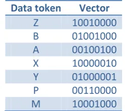
Using a CMM to perform rule-chaining allows for the proposed parallelism of the depth-first search, whilst solving the issues that a conventional system would face. Operation of the CMM for this purpose is no different to a generic CMM as described in Section 2.5. Each token is assigned a unique vector, as shown in Table 6 (in this example using a vector length of 8, vector weight of 2, and generated using Baum’s algorithm):

Data token Vector

Z 10010000 B 01001000 A 00100100 X 10000010 Y 01000001 P 00110000 M 10001000

(24)

[image:24.595.240.356.198.311.2]

In the case that a rule contains a conjunction, either in the antecedent or the consequent, each individual token is assigned a unique vector and the conjunction is simply the logical OR of these. For example, rule 6 within Figure 14a contains the conjunction 𝑃𝑃 ∧ 𝑀𝑀. Using the vectors assigned in Table 6, the conjunction would be represented as 10111000.

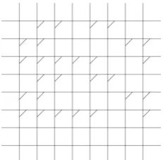
Training of the CMM is performed as in Section 2.5.1, with the only difference being the possibility that input or output vectors may not all have the same weight due to the existence of conjunctions. A CMM trained with the example rule set is shown in Figure 15.

Figure 15: Correlation matrix memory trained with example rule set

Input vector Output vector

10010000 01101100 01101100 11111011

Table 7: Tree search performed on the example

It can be seen in Table 7 that the tree search was indeed conducted rapidly and in parallel, as only two passes through the CMM were required. It is also clear, however, that although the final result is technically correct (the logical OR of tokens 𝑋𝑋, 𝑌𝑌, 𝑃𝑃 and 𝑀𝑀 is in fact 11111011) it is not useful. It is impossible to distinguish which of the tokens comprise the final result, the only certainty is that the vector for 𝐴𝐴 is not included.

This then is one of the problems posed by performing rule-chaining within a CMM – to maintain the separation of multiple tokens within a state to allow them to be individually recognised [1]. The only viable solution to this particular issue is the use of tensor products, as described in the following section.

2.6.3 Tensor products

(25)

a: CMM representation b: Block representation Figure 16: Tensor product of token Z with state S0

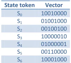
An ideal vector with which to tensor a data token within this system is the state token – these are the labelled branches taken from Figure 14b. Each state token can be assigned a unique vector, however as the data tokens and state tokens are entirely separate it is acceptable for a state token to be assigned the same vector as a data token. The example set of states with assigned vectors is given in Table 8.

State token Vector

[image:25.595.236.359.332.442.2]

S0 10010000 S1 01001000 S2 00100100 S3 10000010 S4 01000001 S5 00110000 S6 10001000

Table 8: State tokens with assigned vectors

a: Tensor product of token B with state S1

b: Tensor product of token A with state S2

c: Superposition of tensor products Figure 17: Superposition of tensor products

A superposition of multiple tensor products remains as simply the logical OR, however as can be seen in Figure 17c, it is now possible to visually distinguish each of the data tokens. More importantly, it is also possible for the system to distinguish each of the data tokens whenever this is required. This requires a two-stage process, as follows:

1. Determine the state tokens that are present in the tensor product

(26)

The use of tensor products resolves the original issue – to allow for the superposition of multiple tokens, whilst maintaining the ability for each of the tokens to be individually recognised. Unfortunately it also exacerbates the issue of matrix size, originally discussed in Section 2.5.5.

Length Weight Section lengths Maximum possible vectors

21 2 {10, 11} 110

64 2 {31, 33} 1023

201 2 {100, 101} 10100

Table 9: Lengths and weights to allocate a given number of vectors

Consider, for example, a system designed to store 100 rules, containing a possible 1000 tokens. Table 9 shows the vector lengths required in the best possible case, and using Baum’s algorithm to allocate vectors to each of the state and data tokens. Each input and output vector would have a length of 21 × 64 = 1344 bits, meaning the CMM would be 13442_{= 1806336}_{bits, or around} 221 kilobytes.

Although 221 kilobytes is not particularly large, consider now a system designed to store 1000 rules, containing a possible 10000 tokens. Each input and output vector would have a length of

64 × 201 = 12864 bits, meaning the CMM would be 128642_{= 165482496}_{bits, or around}

20 megabytes. This is two orders of magnitude larger, and the trend continues in a virtually linear fashion as the number of rules and tokens increases, to the extent that such a system is infeasible for use with large datasets.

There has not been a large amount of research into this area, and as such only one viable solution has been proposed – to separate the storage of antecedents and consequents into different matrices [1].

2.6.4 Two-layer correlation matrix memory

Figure 18 shows a simple block diagram representation of the operation of a two-layer implementation, where the states labelling each of the branches in Figure 14b are used as a link between the first and second CMMs. This does not have to be the case, but is a simple method of assigning a unique label to each rule.

Figure 18: Simple two-layer CMM

The output of this system is designed to be in a format ready to be passed immediately back into the antecedent CMM in order that rule-chaining occurs with only a very simple control system.

(27)

In order to train the two-layer network, the rule set must be modified in order that each rule contains an antecedent, a consequent, and additionally an intermediary state. The previously used example rule set with this adaptation is given in Figure 19.

Antecedent correlation matrix memory

Figure 20: Recall of a tensor product

Training of the first CMM proceeds in the same way as it would with any other single-layer CMM system described in Section 2.5.1, using the antecedent as an input and the state as an output. Recall from this CMM is also performed using a standard method, as described in Section 2.5.2, except that the input in this system is a tensor product rather than just a vector. It is proposed in [1] that each column of the tensor product is individually passed as an input to the CMM. This is shown in Figure 20, where the CMM has been trained with the example rule set. The output is labelled as 𝑆𝑆1∨ 𝑆𝑆2 to indicate that the vector contains the logical OR of 𝑆𝑆1 and 𝑆𝑆2.

It is suggested that Willshaw’s method of thresholding be used, with a value equal to the weight of the input vector during training. This will ensure that all rules that have been trained will be recalled, although if the CMM is heavily populated it is possible that extra rules will also fire [6]. Consequent correlation matrix memory

Figure 21: Undistinguishable recall of superimposed states

(28)

[image:28.595.240.354.73.157.2]

1. 𝑍𝑍 → 𝑆𝑆1→ 𝐵𝐵:𝑆𝑆1 2. 𝑍𝑍 → 𝑆𝑆2→ 𝐴𝐴:𝑆𝑆2 3. 𝐵𝐵 → 𝑆𝑆3→ 𝑋𝑋:𝑆𝑆3 4. 𝐵𝐵 → 𝑆𝑆4→ 𝑌𝑌:𝑆𝑆4 5. 𝐴𝐴 → 𝑆𝑆5→ 𝑌𝑌:𝑆𝑆5 6. 𝐴𝐴 → 𝑆𝑆6→(𝑃𝑃 ∧ 𝑀𝑀):𝑆𝑆6

Figure 22: Two-layer example rule set with tensor products

The solution to this problem suggested in [1] is that the second CMM should instead store correlations between a state and the tensor product of the consequent with that state. To demonstrate this, the example rule set is adapted once more in Figure 22. Training the CMM is then a matter of presenting the state as an input and the tensor product of the state and the consequent as an output.

Figure 23: Correct recall of superimposed states

The recall operation for the second CMM is similar to that for the first CMM; each column of the state tensor product is passed as an input in turn. The output for each column, however, is an entire tensor product as shown in Figure 23. A threshold is applied to each of these output tensor products, and then they are summed – taking a logical 1 to be the value 1 [1]. A threshold can then be applied to the result of this sum, using Willshaw’s method with a value equal to the weight of a state vector. This final tensor product can then be directly applied as an input to the antecedent CMM, in order to continue the rule chaining.

Complete rule-chaining system

[image:28.595.155.444.269.529.2]

(29)

[image:29.595.76.525.71.416.2]

Figure 24: Complete two-layer CMM rule-chaining system (adapted from [1])

The operation of the system is as follows, where numbers refer to Figure 24: 1. A tensor product (1) is presented as an input to the antecedent CMM

2. A threshold is applied to the output of this CMM (2), which is then presented as an input to the consequent CMM

3. Each column in (2) will generate a complete tensor product, for example 𝑆𝑆3∨ 𝑆𝑆4 will generate (3a) and 𝑆𝑆5∨ 𝑆𝑆6 will generate (3b); a threshold is applied to each of these individual tensor products

As there are two copies of 𝑆𝑆3∨ 𝑆𝑆4, there will be two copies of (3a) generated, and likewise for (3b) – this duplication is not shown in the figure

4. All of the output tensor products are summed, with a logical 1 within a tensor product equating to the value 1 for the purposes of addition (4)

5. A threshold is applied to this tensor product, to retrieve the final output (5)

6. In order to continue with rule-chaining, (5) can be presented as an input to the antecedent CMM

Arity networks

(30)

To illustrate the problem, consider a system containing the rule set in Figure 25. If the system is presented with an input of 𝐴𝐴, then rules 5 and 6 would be expected to match. In order for this to be the case, the threshold value would need to be set to the weight of a single input token. This would also allow rule 7 to partially match, and generate an output containing 𝐷𝐷 [1].

1. 𝑍𝑍 → 𝐵𝐵 2. 𝑍𝑍 → 𝐴𝐴 3. 𝐵𝐵 → 𝑋𝑋 4. 𝐵𝐵 → 𝑌𝑌 5. 𝐴𝐴 → 𝑌𝑌 6. 𝐴𝐴 → 𝑃𝑃 ∧ 𝑀𝑀 7. 𝐴𝐴 ∧ 𝐶𝐶 → 𝐷𝐷

Figure 25: Example rule set for arity networks

The solution proposed by [1] is to use a system containing multiple arity networks (Figure 26) Prior to training a rule into the system, the arity is checked and the rule is trained into the appropriate CMM.

Figure 26: Arity networks

Recall from all of the CMMs is able to be executed in parallel, and each of the different CMMs can threshold their outputs with a different value appropriate for their arity. Superimposing the outputs of the various CMMs gives the final output, containing no partially matched rules. This output can then be presented as an input to the system if required.

2.7 Final considerations

(31)

3 Initial planning

It was decided that an iterative development process should be used for this work, as it allowed the addition of functionality in an incremental fashion. Careful planning was required in order to successfully apply the iterative development process to this work. This planning stage was used to decide on the experimentation to be performed during each iteration, and hence the functionality required. Performing an iterative development also aided the testing process, by simplifying the implementation at each stage

Although the AURA library was available for use within this work, it was decided that fully developing a simple implementation without the use of an external CMM library would result in a deeper understanding of the CMM rule-chaining architecture and the techniques used to improve recall reliability.

To this end, five stages were identified that would give a logical progression from the development of a simple CMM to the final demonstration system capable of rule-chaining and online training. The functionality required, and experimentation performed, at each of these stages is described in detail within the next five chapters:

4. Vector recall

5. Tensor product recall

6. Rule-chaining with tensor product recall 7. Superposition of tensor products 8. Use of a two-layer network

(32)

4 Vector recall

4.1 Overview

This first iteration was intended to demonstrate the operation of a simple CMM, with the ability to train and recall vector correlations. As such, this work experimented with the storage capacity of a CMM that has input and output vectors with a fixed length and weight. As well as verifying the correct operation of the CMM, this work investigates the effect of changing the threshold method used and different means of generating vectors, to determine the effects of using Baum’s algorithm rather than a random generation.

4.2 Design

As described in Section 2.5 and [1], a binary CMM is required to store the correlations between an input and an output vector. A CMM is therefore a two-dimensional 𝑃𝑃×𝐶𝐶 matrix which may be stored with a Boolean data type, as a location within the matrix may be either set (at logical 1) or unset (at logical 0).

Creating a class for the CMM allows the main operations of training and recall to be properly encapsulated. In preparation for later iterations of the development process it also allows the use of two separate CMMs, as training or recall operations on one matrix will be independent of any other matrix.

Neural networks and CMMs are known to be applicable to uncertain and fuzzy reasoning, including applications such as pattern recognition [44]. For the purposes of inference, it may be desirable for a system that is capable of reasoning under uncertainty. Alternatively, it may be preferred that the system is able to be certain that any derived consequences are logically entailed by the provided antecedents. As such, the experimentation performed used the premise that an incorrect recall was defined as an output vector that did not exactly match the trained vector.

This work consisted of two experiments, firstly to determine the probability of recall error for a CMM with a fixed input and output vector length and weight, and then to investigate the capacity of a CMM with varying vector weights. As a corollary, this also investigates the effect of changing the methods used for generating vectors and applying a threshold after a recall operation.

Both experiments in this iteration were run 20 times, with the mean results used for evaluation. 4.2.1 Probability of recall error

Using a random vector generation gives no guarantee as to the Hamming distance between vectors. With an improved Hamming distance, as provided by using Baum’s algorithm [8] (described in Section 2.5.3), the capacity of a CMM is expected to increase as the interference between vectors is decreased.

(33)

As Baum’s algorithm is deterministic, different seed values are used for each execution of the experiment. It was decided that although it has been shown that using L-wta to threshold can improve the storage capacity of a CMM [21], it would not be appropriate for this application. When performing rule-chaining, it is likely that there will be multiple rules with the same antecedent. Where this is the case, the output should contain both consequents superimposed. Using L-wta could potentially favour one of the rules over another, resulting in an undesired pruning of the search space. For this reason, only L-max and Willshaw’s thresholding will be compared.

In this experiment, a recall error is defined as an output vector that does not exactly match that which was trained. The operation of this experiment is as follows:

1. Create two identical matrices – one to store randomly generated vectors, and one to store vectors generated using Baum’s algorithm

2. Randomly generate a new input and output vector pair, and ensure that they are unique within the randomly generated system

3. Train the first CMM with this vector pair

4. Generate a new input and output vector pair, using Baum’s algorithm 5. Train the second CMM with this vector pair

6. Recall every previously trained input vector of the first CMM in turn, comparing the output vector to that which was trained

a. Threshold the output pattern using Willshaw’s method b. Threshold the output pattern using L-max

7. Recall every previously trained input vector of the second CMM in turn, comparing the output vector to that which was trained

a. Threshold the output pattern using Willshaw’s method b. Threshold the output pattern using L-max

8. Record the rates of recall error and continue from 2 if any of the results has a rate of recall error less than 100%

4.2.2 Changing vector weight

Using input and output vectors with a greater weight will increase the number of correlations to be stored within the CMM for every vector pair that is trained. It is possible, however, that this increased number of correlations required to meet a threshold may serve to counteract the interference within the matrix.

As such, this experiment is designed to investigate the effect of increasing the weight of vectors stored within a CMM. The results of this experiment may then influence the decision as to the vector weight used for future development iterations. The operation of this experiment is as follows:

1 Create an empty matrix

2 Randomly generate a new input and output vector pair, ensure that they are unique within the system, and train the matrix with this pair

3 Recall every previously trained input vector in turn, using Willshaw’s method to threshold and comparing the output vector to that which was trained

(34)

4.3 Implementation

The CMM is implemented as a class, containing various fields and methods. Using a class in C++ also allows for a destructor to be defined, which is used to free any memory that has been dynamically assigned for the CMM.

Vectors and output patterns (before a threshold is applied) are defined as structures, in order to incorporate important parameters such as their length as well as an array. They are not required to be full classes, as they have no methods that require encapsulation.

A class named vectorGenerator was created in order to create vectors to be stored in a CMM. Although this could have been implemented using functions rather than a class, it was decided that the use of a class would simplify any experimentation. Once the class is instantiated, generating a new vector is a matter of calling a method within that object.

Finally, a rule structure and rules class were created to store any rules that are trained into a particular CMM. This is to allow the system to compare a vector that is recalled from a CMM with the vector that was originally trained; effectively this is using the classical rule storage method of a list in order to test the correct operation of a CMM.

With regards to the implementation of experiments, only a simple control structure is required – firstly defining any variables to be used, and then using loops to train and recall vectors in the CMM.

4.4 Testing

Unit testing was undertaken to ensure that all classes and functions were correctly implemented. Each unit was tested with various test cases, designed to confirm the correct operation of the unit, with the expected results being manually calculated before each test was executed. The complete set of test cases for this development iteration are given in Appendix 2.

Having ensured that all units operated as expected, testing the implementation of the experiments required using the debug facilities of Visual Studio to ensure that the control loops were executed as expected and that variables were declared within the correct scope.

4.5 Results

4.5.1 Probability of recall error

When displaying the probability of recall error from a CMM, it is common to give the number of vector pairs that may be stored and recalled with various probabilities of error [21]. This is due to the possibility that a given probability of error is acceptable within a system.

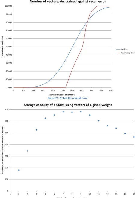
Table 10 shows the number of vector pairs that may be stored to achieve the probability of error given as a column heading, using different methods of vector generation and threshold. The full results are represented graphically in Figure 27.

0% error 0.1% error 1% error 5% error 10% error

Random generation, Willshaw threshold 424 650 1081 1605 1902

Random generation, L-max threshold 424 650 1081 1605 1902

Baum generation, Willshaw threshold 2668 2669 2681 2736 2808

(35)

[image:35.595.72.522.76.736.2]

Figure 27: Probability of recall error

(36)

4.5.2 Changing vector weight

This experiment was designed only to investigate the capacity at which a CMM failed to achieve perfect recall reliability, and as such Figure 28 shows the number of vector pairs that may be stored before any recall fails. A table of these results is given in Appendix 3.

4.6 Evaluation

It was expected that generating vectors using Baum’s algorithm would increase the storage capacity of a CMM, due to the increase in Hamming distance between vectors leading to a reduction of interference. As can be seen in Table 10, and more clearly in Figure 27, this is indeed the case. It can also be observed from the graph that although a CMM storing randomly generated vectors fails earlier than one storing vectors generated using Baum’s algorithm, it also fails at a slower rate. Due to the determinism of Baum’s algorithm, this is to be expected; when the CMM reaches capacity, it is guaranteed that every further vector pair trained into the CMM will cause interference with at least one vector pair that has previously been trained.

Somewhat unexpectedly, the threshold method applied did not affect the recall reliability of a CMM, as both L-max and Willshaw’s methods achieved exactly the same probabilities of error. This inability to distinguish the threshold methods is the reason that Figure 27 shows only two lines; one line for randomly generated vectors, and one for vectors generated using Baum’s algorithm. Threshold methods are discussed in [7], where it was found that when presented with a noisy input, using L-max gave a higher recall reliability than using Willshaw’s method. In this experiment all inputs are exactly as they were initially trained, and so L-max does not provide any benefit.

(37)

5 Tensor product recall

5.1 Overview

A tensor product is formed by taking the outer product of two vectors, and the use of tensor products allows superposition of data tokens within the input or output of a CMM [1]. Having demonstrated the correct operation of a basic CMM, this iteration was developed to extend the recall functionality to include tensor products.

In [3] it is suggested that a CMM be trained using stacked tensor products, i.e. each column of the tensor product is stacked on top of the others, resulting in a single vector. A recall simply requires presenting the stacked input tensor product. On the other hand, [1] proposes a CMM that is trained using only the original input and output vectors. In this process, the recall operation requires iterating through the tensor product, presenting each column as an input to the CMM.

Without the use of a sparse matrix representation, the first method is infeasible due to the very large amounts of memory that would be required. Later iterations of the development process will require a second CMM that is recalled by iterating through a tensor product. This means that although the use of the second proposed method requires more recall operations, any benefits in terms of speed provided by using the first method would be negligible because of the requirement for the second CMM to use the second method. As such, this work investigates the operation of only the second alternative.

5.2 Design

This iteration adds the functionality of recall from a CMM using a tensor product. This is an important aspect of the final system, as it is used to allow superposition of vectors within an input or output while maintaining the ability to distinguish them.

This work consisted of a single experiment, to compare the probability of recall error for a CMM using tensor product recall with one that used basic vector recall. As the recall operation using a tensor product is merely a vector recall applied multiple times, it was expected that the probability of error would also be the same.

5.2.1 Probability of recall error

From the results found in the previous iteration, it was clear that a vector length of 500, using Baum’s algorithm to generate vectors, was sufficient to store a large number of vector pairs. The second experiment that was undertaken showed that with this vector length, a vector weight of around 7 to 9 would give the highest capacity. It was decided, however, that the capacity offered by using a vector weight of 5 would be more than sufficient for this experiment. This has the benefit of allowing the results from the first experiment to be used in comparison to the results of recall using a tensor product.

‘Quantum’ Parallel computation with neural networks

Department of Computer Science, University of York

Submitted in part fulfilment for the degree of MEng

Nathan Burles

10 May 2010

‘Quantum’ Parallel computation

Abstract

Table of contents

List of figures

List of equations

List of tables

1

Introduction

1.1

Aims

1.2

Report structure

1.3

Statement of ethics

2

Literature review

2.1

Finite state architectures

2.2

Rule-chaining

2.3

Quantum computation

2.4

Neural networks

2.5

Correlation matrix memories

2.6

Rule-chaining in correlation matrix memories

2.7

Final considerations

3

Initial planning

4

Vector recall

4.1

Overview

4.2

Design

4.3

Implementation

4.4

Testing

4.5

Results

4.6

Evaluation

5

Tensor product recall

5.1

Overview

5.2

Design