Transformation methods in nonlinear programming

TRANSFORMATION METHODS

IN

NONLINEAR PROGRAMMING

BY

D.M. RYAN

A thesis submitted to the Australian National University for the degree of Doctor of Philosophy.

Acknowledgement (i)

Preface (ii)

Abstract (iii)

Chapter 1 : Introduction

1.1 Problem Description 1

1.2 Transformation Methods for Constrained

Problems 7

1.3 Scope of the Thesis 11

1.4 Definitions and Classical Results 14

Chapter 2 : Barrier Function Methods

2.1 Introduction 26

2.2 Trajectory Analysis and Error Estimates 31 2.3 A New Family of Barrier Functions 40

2.4 Numerical Results 46

2.5 Hessian Conditioning and Computational

Problems 57

Chapter 3 : Penalty Function Methods

3.1 Introduction 62

3.2 The Schmit-Fox Method and Morrison's

Method 63

3.3 The Tangent Parameter 71

3.4 An Algorithm 76

3.5 Numerical Results 80

3.6 Powell's Method 86

Chapter 4 : A Hybrid Method

4.1 Introduction 95

4.2 Equality Constrained Barrier Function

Transformations 96

4.3 Inequality Constraint Classification 104 4.4 Active Constraint Transfers 107

4.5 Hessian Corrections 111

4.6 The Hybrid Algorithm 116

4.7 Numerical Results Using the Hybrid

Algorithm 118

Chapter 5 : Unconstrained and Linearly Constrained Methods

5.1 Introduction 128

5.2 Unconstrained Methods 129

5.3 Projection Methods for Linearly

Constrained Problems 133

5.4 A Hybrid Projection Algorithm for

Minimizing T(x,0,a,r) 139

5.5 Numerical Results 146

I am particularly indebted to my wife, Ruth, for her support, encouragement and longsuffering - attributes that have received a great deal of exercise especially during the preparation of this thesis.

I wish to thank Dr. M.R. Osborne for his

encouraging and stimulating supervision during my three years of study at the Computer Centre, Australian

National University. I am particularly grateful for his interest and the frequent discussions that have led to much of the work presented in this thesis. I would also

like to thank Dr. R.S. Anderssen, first for his super­ vision during the past nine months and secondly, for his constructive criticism of the early version of the thesis.

I also wish to thank Mrs. Stephanie Larkham, whose patience and undoubted skill are clearly evident

in her preparation of the typescript. I am also grateful to Mr. L.S. Jennings for his careful reading and checking of the typescript.

Finally, I would like to thank the Australian National University for the financial support of a

(ii)

PREFACE

Many of the results described in this thesis have been established during or as the result of

collaboration and discussion with M.R. Osborne and have subsequently been published in the following joint papers Kowalik, Osborne and Ryan (1969) and Osborne and Ryan

(1970a, 1970b). When discussing these results in this thesis the text of the relevant papers has been closely followed.

In presenting the basic theory of barrier function methods in Chapter 2, repeated reference is made to Fiacco and McCormick (1968) which can be taken as a standard reference for transformation methods. The reader is referred in Chapter 5 to the original source references for the theoretical properties of the unconstrained and linearly constrained methods discussed. Emphasis in this chapter is on the computational

properties of the methods with particular reference to their use as a computational tool for transformation methods.

ABSTRACT

This thesis investigates a number of

difficulties associated with the design and implement­ ation of transformation methods for the solution of the continuous mathematical programming problem,

minimize f (x) , X £ E ,„n subject to g^(x) ^ 0 , l=T7I,

and h - (x) = 0 , II 1-1 E

where the problem functions f(x), g^(x), t=l,£,

h - (x) , 1=1,m, are at least continuous. The aim is to improve convergence properties of current transformation methods by designing modified methods which avoid the computational difficulties.

In Chapter 2, barrier function methods (interior-point methods) are investigated and a new family of barrier functions, exhibiting improved

convergence properties, is proposed. The theoretical and computational aspects of two penalty function methods (exterior-point methods) are then considered in Chapter 3. Based on the properties of the barrier and penalty function approaches discussed in the

(iv)

constructed in Chapter 4. The theoretical validity of the new approach is established and it is shown

that under mild conditions on the problem (e.g. the Kuhn-Tucker conditions) the computational difficulties of the parent methods are avoided and improved

convergence properties are evident. For problems not satisfying such conditions, the hybrid method behaves as a barrier function method. In Chapter 5, uncon­ strained methods and projection methods for linearly constrained problems are considered and numerical evidence is presented to suggest that if linear

INTRODUCTION

1.1 Problem Description,

The general optimization problem to be considered in this thesis is the mathematical programming problem:

Problem 1.1 : minimize f (x) (1.1)

subject to > o , l=TTZ , (1.2)

and h * (x)

'C ~ = 0 , 1=1,m , (1.3)

where f (x) , the objective function, and g^(x), - i = l ,

and h ;(x), i=l,m , the constraint functions, are real- valued functions of a vector x in the n-dimensional

Yl

vector space E . It will be assumed throughout this thesis that the problem functions, f (x) , g^(x), -1=1,t, and h - (x) , -1=1 ,m, are at least continuous and further restrictions, in the form of differentiability

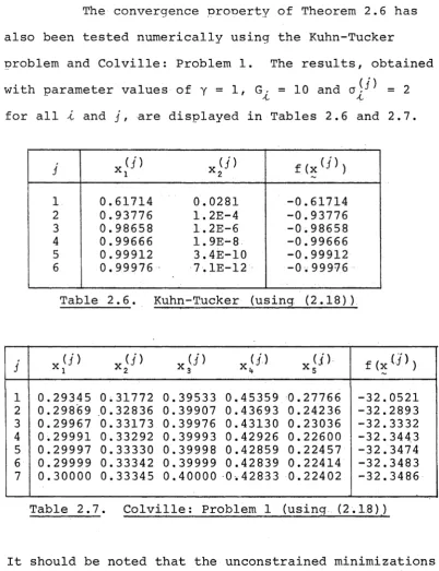
conditions, will be imposed when necessary. It should be noted that the convention of adooting the minimization

advent of modern computers and advances in many fields

of application including operations research, economics,

applied mathematics and industrial design and control.

In the development of theory and solution methods for

Problem 1.1, some classes of the general problem have

proved more tractable than o t h e r s . A number of these

classes will now be described and the development of

theory and solution methods, applicable to each form,

will be briefly surveyed.

The linear programming pro b l e m , where all

problem functions are linear, has been widely treated

since Dantzig (1951) developed the Simplex Method and

an extensive literature now exists. A report of the

basic developments can be found in Dantzig (1963) .

Much of the recent interest has centred on adaptions

of the basic methods to linear programming problems

with special structures.

The linearly constrained problem, Problem 1 . 2 ,

with all constraint functions linear in x has been

studied in two forms:

(i) Quadratic Objective Functions.

Contributions to quadratic programming have

been made by Beale (1959), Wolfe (1959),

Dorn (1960), Lemke (1962), Murray (1969a) and 2 .

(ii) Convex and General Nonlinear Objective Functions. Results and solution methods relating to convex and general nonlinear forms have been developed by Beale (1955), Rosen (1960),

Goldfarb and Lapidus (1968), Fletcher (1968), Goldfarb (1969b) and Murtagh and Sargent (1969).

In the last two decades, the convex programming problem with f(x) convex, g . (x) , 1=1,1, concave and

h - (x) , 1=1,m , linear has received considerable 'L ~

attention. Using the convexity/concavity and the implied "smoothness" of the problem functions,

powerful existence and uniqueness results concerning problem solutions have been derived. The original contributions are due to John (1948), Kuhn and Tucker

(1951), Arrow and Hurwicz (1956) and Arrow, Hurwicz and Uzawa (1958), but many more recent results and methods have appeared, among them Charnes and Lemke

(1954), Frisch (1955), Cheney and Goldstein (1959), Kelley (1960), Zoutendijk (1960), Wolfe (1961), Pietrzykowski (1962), Fiacco and McCormick (1963, 1964a, 1967, 1968), Hartley and Hocking (1963),

Hadley (1964), Geoffrion (1966, 1967), Fiacco (1967), Mangasarian and Fromowitz (1967) and Zangwill (1969).

4 .

require only local knowledge about the problem.

However, convexity, and consequently the results and methods of convex programming, can often be applied in a local sense. Three important forms of the nonlinear problem require independent analysis.

Problem 1.3 e Problem 1.1 with 1=0, m^O. Problem 1.4 = Problem 1.1 with 'tk O s ii o

Problem 1.5 = Problem 1.1 with ii _{o 2} 11 _o

In this thesis, the central investigation will be a detailed examination of transformation methods for Problem 1.3 and Problem 1.4. A brief survey of some typical transformation methods is given in §1.2.

In §1.3, the structure and motivation of the thesis are outlined.

Before investigating transformation

methods, we shall consider results and methods related to Problem 1.5. The unconstrained problem arises in many applications (Kowalik and Osborne (1968)), and

in particular, plays a vital role in transformation methods for constrained problems. Classes of methods

for Problem 1.5 are now surveyed briefly. They fall naturally into two classes.

(i) Direct Search Methods (Kowalik and Osborne (1968)). Direct search methods do not involve the

when the dimension n is small.

(ii)Gradient Methods (Kowalik and Osborne (1968)).

These methods require first order cartial deriv­ atives of the objective function. The simclest of them, the method of steecest descent (Curry (1944)), has a number of imcortant disadvantages (Forsythe and Motzkin (1951), Akaike (1959), Forsythe (1967), Kowalik and Osborne (1968)) mainly reflected in the poor rate of convergence as the minimum is accroached. In recent years, an extensive literature has acceared on more effective gradient methods which can be broadly class­ ified into two groucs. The older methods develoced and discussed by Davidon (1959), Zoutendijk (1960), Fletcher and Powell (1963), Fletcher and Reeves (1964), Shah, Buehler and. Kemcthorne (1964), Daniel (1967a, 1967b) , Bard (1968), Fiacco and McCormick (1968), Meyers (1968), Goldfarb (1969a,1970), McCormick (1969), McCormick and Pearson (1969), Pearson (1969), Polak and Ribiere

(1969) , Powell (1969b), Broyden (1970a) and Greenstadt (1970) incorcorate, at least comcutationally and often theoretically, a full linear search (i.e. one dimen­ sional minimization) in each iteration. The methods are generally based on a quasi-Newton (or variable metric) accroach and sometimes cossess the additional

6 .

(1968), Murtagh and Sargent (1969,1970), Powell

(1969a,1970) and Fletcher (1969c). The distinguish­

ing feature of these methods is the elimination of

the linear search requirement.

Recently, Huang (1969) has developed a unified

treatment of gradient methods in which all presently

known methods appear as particular cases. Surveys,

comparisons and reviews of direct search and gradient

methods can be found in Spang (1962), Fletcher (1965,

1969b), Box (1966), Rosen (1966), Greenstadt (1967),

Kowalik and Osborne (1968), Powell (1968), Box, Davies

and Swann (1969), McCormick and Pearson (1969), Huang

and Levy (1969) and Bard (1970).

Crockett and Chernoff (1955), Goldstein (1962)

and Fiacco and McCormick (1968) have investigated the

use of Newton's method for function minimization. In

particular, Fiacco and McCormick have considered the

special case of minimizing transformation functions

arising from constrained minimization. Although

convergence properties are exceptionally good for

general problems, the method suffers from the disadvant­

age of requiring explicit calculation and inversion of

the second partial derivative matrix during each

iteration. It will be shown in Chapter 2 that, due to

possible ill-conditioning, such inversions can lead to

1.2 Transformation Methods for Constrained Problems.

Since the basic aim of this thesis is to investigate certain properties of transformation methods for nonlinear mathematical programming, we

shall now discuss the background and an intuitive basis for these methods. The methods are often called penalty function methods, but we prefer to follow Murray (1969c) and reserve this term for a particular class of trans­ formations. The transformation approach reduces the computational process of constrained minimization to that of a sequence of unconstrained minimizations of a transformation function involving the original problem functions and controlling parameters. Much of the

historical and theoretical development of transformation methods is described by Fiacco and McCormick (1968), while practical aspects of problem solving by

transformation methods can be found in Bracken and McCormick (1968).

Two basic classes of transformations exist. (i) Penalty Function Methods.

Penalty function methods, sometimes called "exterior-point methods", are designed to impose an increasing penalty on the transformation

function as any constraint is increasingly violated. The solution of Problem 1.1 is, in general,

8 .

R = {x : g ; (x)>0, 1=1,1; h ;(x)=0, 1=1,m}. (1.4)

~ - 'C ~ ^ ~

Penalty function methods can be designed to handle both equality and inequality constraints. The

first use of these functions was made by Courant (1943) in the context of analysing constrained motion problems. Much later this approach was

generalized to multiple inequality constraints and further developed by Ablow and Brigham (1955),

Camp (1955), Butler and Martin (1962), Pietrzykowski (1962) and Fiacco and McCormick (1967). This

method is now known as the quadratic penalty function method. A more general development of penalty function methods, based on a transformation

T (x, r) = f (x) + r $(g(x),h(x)) (1.5)

where $ is zero if g^(x)>0, ^=1,t, and h^(x)=0, f=l,m, and positive otherwise, has been given by

Zangwill (1967b). The function, T(x,r), is minimized for a positive increasing sequence of

r-values.

Two independent contributions by Schmit and Fox (1965) and Morrison (1968) have investigated the properties of the penalty function transformation

T (x, X) = (f(x)-X) 2

m + E

1=1

for the equality constrained Problem 1.3. In Chapter 3, this transformation will be further developed by deriving improved convergence results and a new computational algorithm.

Another penalty function method for Problem 1.3 has been developed by Powell (1967) and is based on the transformation

m

T(x,0,a) = f (x ) + E o ^ [0^+h^(x)]2 (1.7)

-1=1

where the components of 0 and a>0 are controlling parameters. This method is also examined in some detail in Chapter 3. Further contributions

involving penalty function transformations have been made by Edelbaum (1962), Kelley (1962), Beltrami and McGill (1966), Bellmore, Greenburg and Jarvis (1970) and Haarhoff and Buys (1970). (ii) Barrier Function Methods.

1 0.

earliest reference to these methods was made by Frisch (1955) with a logarithmic transformation based on

£

T (X , r) = f (x ) - r E log [g . (x) ] , (1.8)

i = i ~

where T(x,r) is minimized for a monotonic decreasing null sequence of r-values. This approach was

developed for linear constraints by Parisot (1961) and extended to nonlinear constraints by Lootsma

(1967, 1968a). A second barrier function approach, based on an inverse transformation

*-T(x,r) = f (x ) + r T.g. (x) , (1.9)

1=1

again with T(x,r) minimized for a monotonic

decreasing null sequence of r-values, was originally suggested by Carrol (1961) and later developed by Fiacco and McCormick (1963, 1964a, 1964b, 1966, 1968), Stong (1965) and Pomentale (1965). Other results concerning barrier function transformations have been discussed by Rosenbrock (1960), Huard

(1964, 1967, 1968), Faure and Huard (1966),

Bui Trong Lieu and Huard (1966) , Kowalik (1966) , Tremolieres (1968) , Box, Davies and Swann (1969) , Fletcher and McCann (1969), Allran and Johnsen

Combinations of penalty and barrier function methods have lead to the development by Fiacco (1967) , Fiacco and McCormick (1968) and Lootsma (1968b, 1970) of mixed transformation methods. Such methods are considered further in Chaoter 4.

Recently, Murray (1969b, 1969c), Lootsma (1969, 1970) and Fletcher and McCann (1969) have considered the numerical conditioning of certain barrier and penalty function transformations as

functions of the controlling parameters. These results and their implications are discussed in Chapter 2 and provide motivation for developments later in the thesis.

An interesting and important extension of the transformation approach has been reported by Fiacco (1970) in which the continuity condition for the problem functions is relaxed and a more general description of the constraints is permitted.

1.3 Scope of the Thesis.

In this thesis, a number of difficulties associated with the design and implementation of

1 2.

The implications of these modifications are evaluated, where possible, by numerical comparison with results yielded by the original transformations. All calcul­ ations reported in this thesis were programmed in Fortran and performed in double precision arithmetic on an IBM 360/50 computer at the Computer Centre, A.N.U.

Chapter 1 is concluded with definitions and the development of standard results that will play a basic role in the subsequent chapters. The results include characterizations of the optimal solution in terms of the problem functions.

Chapter 2, based on the work of Osborne and Ryan (1970a), considers, in some detail, the barrier function methods for Problem 1.4. Convergence results are examined and on the basis of improving convergence rates, a new family of barrier functions is proposed. Finally, a number of computational difficulties

associated with barrier function methods are discussed and the new barrier function family is examined

numerically.

The third chapter describes an algorithm, based on the penalty function transformation (1.6),

for solving Problem 1.3. Morrison's method is

modified to provide an automatic starting procedure using the Schmit and Fox method and more rapid

Kelley's device (Kelley (1962)) for transforming

inequality constraints into equality constraints is

used and numerical results of the method are presented.

The results related to transformation (1.6) are taken

from Kowalik, Osborne and Ryan (1969). The third

chapter concludes with a discussion of Powell's method

(Powell (1967)) for equality constraints. Attention

is drawn to conditions under which favourable

convergence rates apply. Results relating to Lagrange

multipliers are also given.

Chanter 4 is devoted to the development of

a new hybrid algorithm for nonlinear orogramming. The

new algorithm is based on the methods and results of

Chapter 2 and §3.5 and §3.6 and is motivated by

(a) the computational problems associated with

barrier function m e t h o d s , and

(b) the excellent convergence properties of

Powell's method.

It will be shown that the hybrid algorithm avoids the

computational difficulties of barrier function methods

and utilizes Powell's method in circumstances which

ensure its rapid convergence. These two features

provide a highly competitive method which is

illustrated by numerical comparisons with a standard

14 .

In Chapter 5, a number of quasi-Newton

methods for unconstrained minimization and two projection algorithms for linearly constrained minimization

(Problem 1.2) will be considered. A modified projection algorithm, based on these methods, will be developed to minimize linearly constrained problems on a subset of

yi

E . Such problems arise in Chapter 4 when using

transformation methods to handle nonlinear inequality constraints.

1.4 Definitions and Classical Results.

This section will discuss the classical results of mathematical programming theory developed originally by John (1948) and Kuhn and Tucker (1951) and later extended by Arrow, Hurwicz and Uzawa (1961). The results involve necessary and sufficient conditions for the existence of local minima in terms of the

original problem functions f (x) , g^ (x) , -1=1,£, and

h^(x), t=l,m. Concepts used in this derivation are due

to Hestenes (1966), but alternative approaches are described by Fiacco and McCormick (1968) and Lootsma

(1970). Attention will be restricted to optimization over Euclidean n-space assuming that all problem

functions are at least continuous. Further restrictions, in the form of differentiability conditions, will be

and sufficient conditions, only major results will be proved but references or outlines of proofs will be provided in other cases.

Definition 1.1. The feasible region, R, for Problem 1.1 is defined by (1.4).

Any x e R is said to be feasible. It is assumed throughout this thesis that R ^ 0 (the empty set). The following definitions provide a character­ ization of minima on R.

Definition 1.2.(i) The function f(x) has a local minimum, x*, on R (i.e. x* e R) iffthere exists 6 > 0 s.t. f (x) > f(x*) for all x e N(x*,6) r\ R where

N(x*,6) = {x : I Ix-x*I I < 6}.

(ii) The local minimum is isolated iff f(x) > f(x*) for all x e N(x*,6) n R, x / x*.

(iii) The local minimum is global on R iff f (x) > f(x*) for all x e R.

(iv) The local minimum is unconstrained iff f (x) > f (x*) for all x e N(x*,6) for some 6 > 0.

fe. fö. H

Definition 1.3. A sequence of ooints {x }, x e E , fe d ^

1 6.

1 a n d x^ ^ x* f o r a l l fe i f f

l i m life *

fe+°° II? “ ?* 1! = 0 a n d

l i m fe-* o o

x -x— V *

X -X— V *

Definition 1 . 4 . The tangent c o n e , C ( x * ) , of R at

x* e R is

h h d

C(x*)= ( X d :X > o , I IdI I=1, there exists (x ;cR s.t.xfe + x*

Definition 1 , 5 . (i) A function, f ( x ) , has a first order

differential at x* iff f(x) is defined in a neighbourhood

of x* and there exists a function f ' (x*,d), linear in d,

fe fed

which, for any sequence {x } s.t. x + x*, satisfies

lim fe -* o o

f (xfe)-f (X*)

f ' (x*,d) .

(ii) A function, f ( x ) , has a second

order differential at x* iff f(x) has a first order

differential at x* and there exists a function

f 1' (x*,d), quadratic in d, which satisfies

f(x^)-f(x*)- f '( x * , x Z- x * ) lim

Remarks 1 . 1 . 1. We may write f (x*,d) = d Vf(x*)

and f '' (x* fd) = dT V 2 f(x*)d where Vf(x*) and V 2 f (x*)

are called the gradient and Hessian respectively, of

f(x) at x * .

2. If f(x) e C ^1^ (i.e. once contin­

uously differentiable) in a neighbourhood of x*, then

f(x) has a first order differential at x* and the

vector, Vf(x*), has as components, the first partial

derivatives of f(x) at x*.

(2 )

3. If f(x) £ C in a neighbourhood

of x*, then f(x) has a second order differential at x*

and the matrix, V 2f( x * ) , has as elements, the second

partial derivatives of f(x) at x*.

Using Definition 1.2, Definition 1.5 and

Remarks 1.1, Lemma 1.1 can be established and describes

first and second order necessary conditions for local

minima on R.

Lemma 1 . 1 .

(i) If f(x) has a first order differential at

x* £ R where x* is a local minimum on R, then

f'(x*,d) = d T Vf(x*) > 0 for all d e C(x*).

(ii) If f(x) has a second order differential at

x* e R where x* is a local minimum on R and Vf(x*) = 0,

1 8.

Sufficient conditions for x* to be a local

minimum on R are now stated in Lemma 1.2. Again the

proof of this lemma follows from Definition 1.2,

Definition 1.5 and Remarks 1.1.

Lemma 1 . 2 .

If f(x) has a second order differential at

x* e R, Vf(x*) = 0 and f ' (x*,d) = dT V 2f (x*)d > 0

for all d £ C ( x * ) , d ^ 0, then x* is an isolated local

minimum on R (i.e. there exist y, 5 > 0 s.t. f(x) >

f (x*) + y I Ix—x * I I 2 for all x £ N ( x * ,6) n R).

The results of Lemma 1.1 and Lemma 1.2 are

now extended by developing a description of C(x*) in

terms of the constraint functions, g - (x) , 1=1, 1, and

h ^ ( x ) , 1=1,m. If x* £ R and g^(x*) > 0 for some 1,

then by the continuity of g^. (x) , it follows that

g.(x) > 0 on a sufficiently small neighbourhood of x*.

This observation implies that the local character of

R at x* and hence C ( x * ) , will be defined by the active

constraints at x*.

Definition 1 . 6 . The set of active inequality

Lemma 1 . 3 .

If d e C(x*) and the constraint functions,

g ; (x) , i £ B(x*) , and h> (x) , -1=1,171, have first order

differentials at x*, then d satisfies

and

g'(x*,d) = d T Vg-(x*) > 0, L £ B(x*), (1.10)

hj.(x*,d) = d “ Vh^(x*) = 0, l = l,m . (1.11)

This lemma states that all directions in the

tangent cone of R at x* are into the feasible region.

Kuhn and Tucker (1951) have constructed a simole

example showing that the converse is not necessarily

t r u e .

Definition 1 . 7 . The point, x*, is a regular point

of R iff for all d satisfying (1.10) and (1.11),

d £ C ( x * ).

A c h a r a c t erization of a regular point, in

terms of the constraint functions, is given by

Lemma 1.4. Extensive discussion and proofs of these

c o n d i t i o n s , known as constraint q u a l i f i c a t i o n s , have

been given by many authors including John (1948),

2 0.

Hestenes (1966), Mangasarian and Fromowitz (1967),

Fiacco and McCormick (1968) and Lootsma (1970).

Lemma 1.4.

Any one of the following conditions is

sufficient for x* to be a regular ooint of R.

(i) The vectors, Vg-(x*), o e B(x*), Vh; (x*),

1 = 1 ,m, are linearly independent.

(ii) There exists d s.t. dT Vg.(x*) > 0,

Ö e B(x*), dT Vh-(x*) = 0, o=l,m, and

~ ~ -'C

Vh-(x*), -0=1,m, are linearly independent.

(iii) The Kuhn-Tucker constraint qualification

(Kuhn and Tucker (1951) , Fiacco and McCormick

(1968)) holds at x*.

This lemma is usually Droved by showing

(i) =>(iii) =>x* is regular and (ii) =>x* is regular.

The following result concerning linear functionals

will also be useful in establishing the required

necessary and sufficient conditions for constrained

optimality.

Lemma 1.5. (Hestenes (1966), o,13).

Let F(x), (x) , -t=l , t , (x) , o=l,m, be

linear functionals on a real linear space X. If

F(x) > 0 for all x e X s.t. (x) > 0, 0=1,t , and

H^(x) = 0, o=l,m, then there exist multipliers

u •, 0=1,t , and v-, 0=1,m, s.t. u- > 0, o=l,t , and

t

m

F (x) E u. G . (x) + Z v. H . (x) = 0

1 = 1 x ^ ~ i = i x ~

for all x e X. Furthermore, if G.(x), 1=1,£,

H ; (x), -1=1,171, are linearly independent, the multipliers are unique.

We now introduce a function which clays an important role in both the classical theory of

mathematical programming and the results of this thesis.

Definition 1.8. The Lagrangian function, L(x,u,v), associated with Problem 1.1, is

£ m

L(x,u,v) = f (x) - Z u . g.(x) + Z v. h . (x) (1.12)

~ ~ ~ ~ ' 1 'C 'C ~ 'C ~

yt=l ^=1

where u e E^ and v £ E171.

Assuming the problem functions have first order differentials, the well known Kuhn-Tucker first order necessary conditions can now be established.

Theorem 1.1.

If x* is a regular point of R and a local

I

m

22 .

g -

> o ,

l=T7£,

'

h^(x*) = 0 ,

l=T7m,

u * g-(x*) = o ,

l=T7T,

u*

> o

'C

and V L(x*,u*,v*) = 0 . (1.17)

X ~ ^ ~

Proof. Since x* is regular, d e C(x*) for all d satisfying (1.10) and (1.11). For d e C(x*), using Lemma 1.1(i), f'(x*,d) > 0 since x* is a local minimum on R. Using Lemma 1.5, we deduce the existence of multipliers u ;, l e B(x*), v*, i - l,m , s.t. u> > 0,

i. e B (x*) , and

m

f ' (x*, d) - £ u- g * (x* ,d) + E v * h (x* , d) =0 ~ ~ -leB (x*)

i=1 *- *■ ~ ~

for all d e C(x*). Defining u£ = u^, t e B(x*), and u* = 0,

i. fL

r ~ x ~ ~ ~

and u* satisfies (1.15) and (1.16).

Remarks 1.2. 1. The vectors u * , v* are called

generalized Lagrange multipliers (GLM) or dual variables. The latter term arises from the theory of convex

2. If x*, a local minimum on R, is not

regular, then the GLM are not all finite.

3. If condition (i) of Lemma 1.4 holds,

then the GLM are unique. This result follows from the

uniqueness result of Lemma 1.5.

Assuming the problem functions have second

order differentials, then the second order necessary

and sufficient conditions may be developed.

Definition 1.9. Let (i) B, (x*) = U h e B(x*) ,ubO},

(ii) R l={x:xeR,g.(x)=0,^sBi (x *)},

and (iii) C l(x*) be the tangent cone of

R at x * .

l

Theorem 1.2.

If x* is a regular point of R and a local

minimum of f(x) on R, then the first order necessary

conditions of Theorem 1.1 are satisfied and, for all

d e C (x*) ,

~ l ~

dT V2 L(x*,u*,v*) d > 0 . (1.18)

Proof. Since L(x,u*,v*) = f(x) on R^ and x* is a

local minimum of f(x) on R , the result follows

l

2 4 .

Remarks 1 . 3 . 1. If d £ (x*), then d £ C(x*) and

d T Vg.(x*)=0, i £ B (x*) .

2. x* is a regular uoint of if

d £ C x (x*) for all d £ C(x*) satisfying- d T Vg^(^)=0,

i £ B 1 (x*) .

3. Sufficient conditions for x* to be

a regular point of R are orovided by Condition (i) of

Lemma 1.4.

Theorem 1 . 3 .

If, at x*, there exist vectors u* and v*

satisfying the conditions of Theorem 1.1 and, for all

d £ C i (x*) ,

d ~V2L(x*,u*,v*) d > 0 , (1.19)

then x* is an isolated local m i n i m u m on R.

P r o o f . Assume that x* is not an isolated local

m i n i m u m on R. Then for every integer, fe, there exists

b h

x £ R, x ^ x * satisfying

||x^-x*|| < ^ and f (x^)-f (x*) <^-1 | x^-x* | | 2 . (1.20)

Iz

From the sequence {x }, a subsequence, also denoted by

D efining the function

m

G(x) = E u* g - (x) E h .(x) XeR(x*) ^ ^ ~ X=1 ^ ^ ~

we note that G(x*)=0 and G(x)>0 for all x e R. For all x e R it follows that

f(x) = L(x,u*,v*) + G(x)

and from (1.20) ,

L(x^,u*,v*)-L(x*,u*,v*) G ( x fe)

< 1

F *

Using (1.17), Definition 1.5 (ii) and Remark 1.1(1) we have

i d T V 2L (x*,u*,v*)d + 1j \ 8" p

G ( x fe) x fe-x*| I 2

< 0 (1.2 1)

and since G(x )^0, the second term is bounded. Therefore

d T V 2L(x*,u*,v*) d < 0 . (1.22)

It also follows from (1.21) and (1.11) that

lim

k-+oo

G ( x fe) Il;fe-;*lI

= G ’ (x*,d) E u* g)(x*,d) X e B l (x*)

0 ,

and since u*>0, isB(x*), then g}(x*,d)=0, ieB (x*) . this implies d e C 1 (x*) and thus, (1.22) provides the c o n t r a d i c t i o n .

2 6 .

CHAPTER 2

BARRIER FUNCTION METHODS

2.1 Introduction.

In this chapter, barrier function transform­ ations for the solution of Problem 1.4 will be studied. For the nonlinear form of Problem 1.4, the solutions generated are local solutions which, for the oarticular case of convex problems, can be shown to be global.

The transformation is written

T (x, r) = f (x) + r $ (g (x) ) , (2.1)

where r is a positive controlling parameter and 4> is a function of the inequality constraint vector g(x) and thus x. Convergence properties, including rates of convergence, will be discussed. The basic theory of barrier function transformations can be found in Fiacco and McCormick (1968).

Here, attention will be restricted to separable transformations of the form

£

4>(g(x)) = Z <p j (g. (x) ) (2.2)

~ ~ t "'L -'C ~

-C=l

with the (j) ■ defined by Definition 2.1.

Definition 2 . 1 . The function cj> , is a barrier function

for g^(x) if

(i) cf>^ is a continuous function of (x) for

x e P-0 where R is the nonemuty interior of R , R given by

(1.4) with m=0.

(ii) (p^(g^(x)) + 00 as g^-(x) ■> 0+.

(iii) <f)^ is a twice continuously differentiable

function of g^(x) for g^(x)>0 (i.e. x e R q ).

(iv) (f>^(g.(x)) satisfies:

(a)

(g^(?))

< ₀ for all x £ R q ,

d 2<p. (gy (x) )

(b) --- > 0 for all x £ R ,

j 2 ~ 0

dg^

d 2 (g^ (x) )

(c) --- is a monotonic decreasing

d g 2

function of g^(x), x £ R .

Remarks 2 . 1 . 1. Conditions (i) and (ii) of

Definition 2.1 are the essential defining orooerties

of a barrier function, while conditions (iii) and (iv)

are only required to establish uniqueness orooerties

for an isolated trajectory of minim i z i n g ooints, x(r),

of (2.1) as r tends to zero. (See Fiacco and

2 8 .

2. The logarithmic barrier function (1.8) and the inverse barrier function (1.9) both satisfy (2.2) and Definition 2.1.

A basis, given by Fiacco and McCormick, for the barrier function methods is provided by the

following lemmas and theorem. Proofs of the lemmas can be found in the references cited.

Lemma 2.1. (Rudin (1953), o.67).

A continuous function on a nonemuty compact set attains its minimum on the set.

Lemma 2.2. (Fiacco and McCormick (1968), d.46).

Let R be a closed set, S a compact set and Ry^S ^ 0. If T(x) is continuous on R0nS with the property that for every sequence {x^} c R QrvS with x^ -* x e (R-Rq )nS, T(x^)=°o, then T(x) attains a finite minimum value on RQr\S.

Lemma 2.3. (Fiacco and McCormick (1968), p.47).

If a set of local minima, A*, corresponding to a local minimum value, f*, of Problem 1.4 is a

nonempty, isolated, compact set of A = {x : f(x)=f*}, then there exists a compact set S such that A* c S and

o

for any point x e RnS such that x £ A * , f(x) > f*

Theorem 2 . 1 . (Fiacco and McCormick (1968), d.47).

If (i) the Droblem functions are continuous,

(ii) each cj)^ satisfies Definition 2.1,

(iii) {r^} is a strictly decreasing null sequence,

and

(iv) there exists a nonempty isolated compact

set, A*, of local minima corresponding to a

local minimum value, f*, such that

A* r\ cl(R ) ^ 0, where cl (.) denotes closure,

then (a) there exists a compact set, S, such that

A* c S Q and for k sufficiently large, the

fz fz

unconstrained local minima, x , of T(x,r )

given by (2.1) exist in R Qn S 0 and every limit

fz

point of any subsequence, {x }, is in A*,

(b)

1

lim k v , , , fz. x

», r E <b . (g .(x ) )

fz-*00 . t ~

y C = l

= 0 ,

(c) _{fei” = f <;*>}

-(d) T(xfe,rfe) = f ( X * ) ,

(e) (f(x^)} is a monotonic decreasing sequence,

and

(f)

l ,

{ E <J> . (g. (xß ) ) } is a monotonic increasing

t = 1

3 0.

Proof. (Fiacco and McCormick (1968), d.48 and d.60). The proof is based directly on Definition 2.1 and Lemmas 2.1, 2.2 and 2.3.

A more general result is available for the transformation

~ k ^ k

T(x,r ) = f(x) + E (g^(x)),

1=1

fz

where {r } is a strictly decreasing null sequence with the orderinq determined comoonentwise.

Theorem 2.2.

If conditions (i), (ii) and (iv) of Theorem 2.1

Iz

are satisfied and {r } is a strictly decreasing null sequence, then conclusions (a), (b), (c) and (d) of Theorem 2.1 remain valid.

Proof. The proof is similar to the proof of Theorem 2.1.

Remark 2.2. Given a sequence of positive vectors tending to zero, it is possible to select a subsequence which is strictly decreasinq. Theorem 2.2 may be

2.2 Trajectory Analysis and Error Estimates.

An imDortant feature of the barrier function

transformation is that a GLM vector, u * , satisfying

the Kuhn-Tucker necessary conditions (1.15), (1.16) and

(1.17) at x * f can be derived from the sequence of

u nconstrained minimizations if either condition (i) or

condition (ii) of Lemma 1.4 is satisfied. For condition

(i) , this result is given by Fiacco and McCormick (1968),

p.73. A constructive proof of the result for condition

(ii) has been given by Beltrami (1969) and an alternative

approach has been discussed by Osborne and Ryan (1970).

Let K ( x * ) be the m atrix w ith columns formed

from the vectors Vg^(x*), i. e B(x*), and assume K(x*)

has rank -6 < n. After reordering the columns, if

necessary, let K(x*) be partitioned into matrices,

K} (x*) w i t h rank 4 and K 2 (x*) , such that K 2 (x*) =

K 1 (x*)U, where U expresses the linear dependence of

columns of K 2 (x*) on columns of K . ( x * ) . Denoting the

matrices formed from the columns of (x*) and (x*) ,

evaluated at x, by K (x) and K 2 (x) respectively, it

follows that the rank of K (x) is 4 if x is sufficiently

close to x*. Finally, define

-t

-rk

>>

3 2.

and let the components of a" and 3 be selected from

k.

the components of u corresponding to the constraints

k. fz

of K (x ) and K (x ) respectively. It should be noted,

1 ~ 2 ~

k

using Definition 2.1, that u., f =1, JL, are bounded below

fc fe

and u^ -> 0 as r 0 for all 4. B(x*) .

Theo r e m 2 . 3 . (Osborne and Ryan (1970)).

fz

If {r } is a strictly decreasing null sequence

fz fz

s.t. x -* x* and the components of 3 are bounded for

/\ /\

every fz > f z , w h e r e fz is sufficiently large, then the

fz fz p

sequence of vectors a + U ß , fz = f z , f z + 1, ...,

converges and

ki™ (afe+ U ß fe) = [Kj (x*)T K 1 (x* ) ] ' 1 K 1 (x*)T Vf (x*) . (2.4)

Proof. Since x^ minimizes T(x,r^),

fz

Vf (xß ) -r

■ i z B (x*)

k )) k fe

— v g^r (x ) + 0 (r ) dg

l

t, , fz, fz , T, , fZ\ nf z , / fZ\

K (x ) a + K (x ) 3 + 0 (r )

i ~ ~ 2 ~

K (xfö) (afe+ U 3 fe)+(K ( x k ) - K (xfe)U)3 ^ + 0 (rfe) . (2.5)

1 ~ 2 ~ 1 ~

But (2.5) is compatible by construction and therefore

(afe+ U ß fe) = [K (xfe)T K (xfe)l 1 K (xfe)T {?f (xfe)

-~ 1 ~ 1 ~ 1 ~

(K ( x f z ) - K ( x f z) U ) ß tz + 0(r^)} .

2 ~ 1 ~

(2.6)

fz

k k

Corollary 1 . If a and $ are bounded for every fe > fe, then there exists a vector, u * , satisfying the Kuhn- Tucker conditions (1.15), (1.16) and (1.17) at x*.

fe

Proof. It does not follow from Theorem 2.3 that a

k

k

k

and 3 converge but, using the boundedness of a and 3 , it is oossible to select a convergent subsequence,

h h

{ (a ,3 )}, with limit (a,3) satisfying

a + U3 = [K (x*)TK (x*)]"1 K (x*) TVf (x*) .

~ i ~ i ~ l ~

When padded out with zeros corresoonding to the inactive inequality constraints (i.e. -I £ B(x*)), the limit

yields the required GLM vector, u*.

Corollary 2 . If the Kuhn-Tucker necessary conditions are not satisfied at x*, then the sequence,

{— (x*) [u£]}, is unbounded as k -* 00.

Corollary 3 . If condition (i) of Lemma 1.4 is satisfied, then there exists a constant, y, s.t

■ceB Oc*) [u2 ] < y for all fe > fe .

Proof. By condition (i) of Lemma 1.4, K(x*) has full rank (i.e. K(x*)=K (x*)) and for k sufficiently large,

~ i ~

k

K(x ), k > fe, also has full rank. It follows from (2.6)

fe

It is now shown that the components of and

k.

3 are bounded if condition (ii) of Lemma 1.4 is

satisfied, and thus, the existence of a GLM vector, u*, is established by Corollary 1 of Theorem 2.3.

34 .

T h e orem 2 . 4 . (Osborne and P.yan (1970)).

If condition (ii) of Lemma 1.4 is satisfied, then there exists a constant, y, s.t.

max ieB(x*)

r fe,

[u^r] < y for all k > k.

P r o o f . For k sufficiently large and using the continuity of the constraint functions,

T . k

d Vg - (x ) > 0

A

L £ B (x*) , k > k , (2.7)

where the existence of d is guaranteed by Lemma 1.4 (ii). At x , a local m i n i m u m of T ( x , r ^ ) ,

Vf(x^) = Z U j Vg . ( x S + O(r^) , i eB(x*)

whence

d T V f( x k ) - 0( r k ) min r,Tn , k, ,

isB(x*) 7gX (? )]

(2 .8)

Z isB (x*)

The desired result follows from (2.9) as each term in the sum on the left is positive and the denominator on the right is bounded away from zero by (2.7) for k > k .

Using the convercrence properties of the GLM

k fz

estimates, u , an error expression for [f(x )-f(x*)] is now developed in terms of the problem functions and the

(z

GLM estimates at x . A second application for the GLM estimates is discussed in Chapter 4.

Theorem 2.5. (Osborne and Ryan (1970)).

If (i) the problem functions are twice continuously differentiable,

fz

(ii) {r } is a strictly decreasing null sequence

fz +

s . t . x x* ,

(iii) the components of u^ are bounded for all fc > fc, and

fz t fz

(iv) (x -x*) Vf(x ) satisfies a strict order relation

(x^-x*)TVf (xS = SO (

I

I

I

I

min |(sfe-S*>TVf(xfe)| ^ ^

k > k

I

then

f(xfe)-f(x*) = + 0 (max [rfö

I

I

I

I

I

I

I

I

36 .

where

E. = £ U j g . (xfe) (2.12)

ß ieB(x*) ^ ^ ~

and the left hand side of (2.11) is S O ([|x^-x*||).

P r o o f . The result follows by taking the scalar

h

product of both sides of (2.8) with (x -x*) and using

the first order Taylor expansions about x* for the

functions. It should be noted that (2.11) is valid

without (2.10) which only ensures that dominates

the right hand side.

Corollary 1 . If cj) . is the inverse barrier function

h I

given by (1.9), then = 0 ( [r ]2 ). If cf)^- is the log

barrier function given by (1.8), then E^ = O(r^).

P r o o f . For the inverse barrier function, under the

conditions of the Theorem, (2.3) implies g^(x^) =

k 1

0 ( [r ]2 ), l e B(x*), and the result follows from (2.12). For the log barrier function, (2.3) implies

fz k.

g^(x ) = 0 (r ), and again the result follows from (2.12).

Remark 2 . 3 . Corollary 1 of Theorem 2.5 implies that,

k

for a given strictly decreasing null sequence { r c},

the log barrier function can be expected to provide a

faster convergence to x* than the inverse barrier

function. This observation motivates, in part, the

The strict order condition (2.10) is related

to the condition of strict c o m p l i m e n t a r i t y ,

u* > 0 for all a. e B(x*) , (2.13)

which is used by Fiacco and McCormick (1968)

(Chanter 6) in a similar context.

Theorem 2.6. (Osborne and Ryan (1970)).

If conditions (i), (ii) and (lii) of

Theorem 2.5 hold, then

(a) for the inverse and log barrier functions,

the strict order condition (2.10), implies the strict

complimentarity condition (2.13), and

(b) for the log barrier function, assuming

Lemma 1.4 (ii) is satisfied, condition (2.13) imolies

(2.1 0).

Proof. (a) Using Theorem 2.5 (i),

If (2.13) is not satisfied, then for at least one

L £ B (x*) ,

for all i e B(x*) so that at most

3 8.

lim k = lim _ k d ^ (gi (? fe))

uf k-+°° r dg^

(2.15)

For the inverse barrier function, (2.15) implies

r^ = 0 ( g . ( x ^ ) 2 ). Using (2.14), r^ = 0 (j |x ^ - x*| j2).

'' C ~ ~ ~

Thus (2.11) becomes

(xfe-x*)TV f( x k ) = 0 ( I Ix^-x*I I) (2.16)

showing that (2.10) is not satisfied.

For the log barrier function, (2.15) implies

r^ = 0(g^(x^)). Using (2.14), r^ = 0 ( ||x^-x*| j).

Thus (2.11) takes the form

(xfö-x*)T V f(xk ) = £ r k + 0 ( j j x fe-x*I j 2 ) (2.17)

f £B (x*)

again showing that (2.10) is not satisfied.

(b) For the log barrier function, the

required result follows from Theorem 15 of Fiacco and

McCormick (1968), p .81, which guarantees the existance

of derivatives of the m i nimizing trajectory, x = x(r),

in a neighbourhood of r = 0, to an order consequent

on the smoothness of the problem functions. Let the

a-order derivative be the first non-vanishing

derivative at r = 0. Then

k

x -x* [r

d a x (0)

a !

n , r f e , a + i ,

and thus , r 1 = SO ( j |x^-x* j j ot) , a > 1. But by (2.17), a = 1 is the only case for which (2.13) holds and thus (2.10) is satisfied.

The error expression (2.12) can be used in a number of ways. First, if the active constraints at x*

(i.e. i. s B (x*) ) can be determined, then (2.12) orovides an asymptotically correct error estimate of

h

[f(x )-f(x*)].Secondly, the sum in (2.12) can be

extended over all constraints and in this case, a bound

Iz

for the error, valid for r sufficiently small, should be obtained. It is known that this bound is strict when Problem 1.4 is convex. For this problem, it can be derived using properties of the dual problem

(Fiacco and McCormick (1968), p.98). As the inactive constraints do not influence the solution, the sum over active constraints also gives a strict bound.

Osborne and Ryan (1970) have treated a number of simple numerical examples to demonstrate the effect of violating the Kuhn-Tucker conditions or conditions

(2.10) and (2.13). They show that rates of convergence of barrier function methods are not necessarily

affected adversely if the Kuhn-Tucker conditions do not hold: but they can be adversely affected if either

2.3 A New Family of Barrier Functions.

Motivated by the observations of Remark 2.3 concerning the inverse and log barrier functions, a new family of barrier functions is constructed with improved convergence properties for a given strictly

fz

decreasing null sequence, {r >. This is achieved by choosing 4> to "reduce" the error, F^, given by (2.12).

If R is bounded, then for 6 > 0, let

G . , J L =1, 1 , be chosen so that

'C

> 1 + 6 + log(g^(x)), 1=1,1,

and if R is unbounded, choose G^ sufficiently large so that when log(g^(x)) > G^ - 1, g^(x) can safely be ignored in any reasonably scaled problem. Let

„ G - -1 - 6

R = {x : x eRq; 0 < g^(x) < e , 1=1,t , 6 > 0}.

Remarks 2.4. 1. If G ; = 10, then g ;(x) can take

— —— —— — —— —— — —— /(_ 'C ~

A

values of order 10H on R and, in particular, near the

minimum of the transformation function. Such a constraint is unlikely to be violated under these conditions if

the problem is reasonably scaled.

/s

If R is bounded, then R = R .

' o

40 .

Define, for x e R ,

(1)

(g^ (x) )=log [G^ - log (g^ (x) ) ]

U = l 7 7 , (2.18)

<pjj +1) (g^ (x) ) = l o g [ a j j } +(pjj * (g^ (x)) ] , j = l, 2 , . .

( J )

w h e r e a- > 1, -1=1, £, / = 1 , 2 , . . , and w r i t e

l

<P(J> (g (x) ) = Z (j.!^ (g. (x))

L=1

(2.19)

T h e n the f a m i l y of f u n c t i o n s , $ ^ ( g ( x ) ), j = l , 2 , . . ,

are b a r r i e r f u n c t i o n s in the f o l l o w i n g r e s t r i c t e d sense.

L e m m a 2 . 1 .

W r i t i n g <J> ^ for (j) ^ (g . (x) ) and g - for

g ^ ( x ) , then

(a) the f u n c t i o n , > s a t i s f i e s D e f i n i t i o n 2.1

A

on R,

(1 )

( J )

(b) the f u n c t i o n s , (fOJ , j =2,3,.., s a t i s f y

p r o p e r t i e s ( i ) , ( i i ) , (iii) and (iva) of

D e f i n i t i o n 2.1 on R and

(c) ^ ca n be c h o s e n so t h a t (f)M + ^ , j = 1,2, . . , /\

is c o n v e x on R (i.e. s a t i s f i e s D e f i n i t i o n

2.1 ( i v b ) ).

P r o o f . D e f i n i t i o n 2.1 ( i), (ii) an d (iii) are

( J )

o b v i o u s l y s a t i s f i e d b y (p , j = l , 2 , . . , on R.

''C

-1 1

42 .

dcj)(/)

4 j-1

_n

d g

4 [G^-log ( g j ] 4 = 1 o ^ >)+<p^

(4 )■, j =1,2 , . . , (2.20)

dcj)(1 )

and for x e R an d o- > 1, — --- < 0, j-1,2,.., thus

* d ^

A

s a t i s f y i n g D e f i n i t i o n 2 . 1 (iva) on R and e s t a b l i s h i n g p a r t (b) of the Lemma. P a r t (a) of the L e m m a is v e r i f i e d by e x a m i n i n g the o r o p e r t i e s of

on R. P a r t (c) of the L e m m a is

,2,(1) d

t

and dg

4 dg4

p r o v e d i n d u c t i v e l y u s i n g the c o n v e x i t y of (p^

e s t a b l i s h e d in (a). F r o m (2.18),

(1)

d 2 c|)ji + 1 ) 1 f d 2 4>

U

)

y 4 1

rd*(/)i

2

-d g 2-

o^ ^

+<P^

^

4 Y 4 - d V - _

d **iy)

> 0 for x e R, t h e n --- —--- > 0 for dn

x e R iff

dg -4

a 0'> > m a ?

4 X £ R

d *4 U h dg 4

2 As)

d <f) . Y4 d g 2

4

- 0(/> 4

(/) 4

and thus a = m a x [ l , + e] , e > 0, is c h o s e n to e n s u r e the c o n v e x i t y of a s s u m i n g cf>^ ^ is c o n v e x

4

It s h o u l d be n o t e d t h a t S .

4

Remarks 2.5. 1. As g

■L o,

j — 1 , 2, . . ,

therefore, on a small enough neighbourhood of x*,

1, /=1,2,.., e B(x*), can be expected to

preserve convexity.

(/)

2. The functions, (p^J , j=2,3,.., need not satisfy Definition 2.1(ivc). This is not

serious disadvantage, since this property is not

required for the basic convergence results of the

barrier function methods.

(1 )

3. For d) ' , if the strict order

condition (2.10) is satisfied under conditions (i)

(ii) and (iii) of Theorem 2.5, then the strict

complimentarity condition (2.13) is satisfied.

Using (2.18), (2.15) becomes

lim

k-yoo

k

__________ r___________

g^(xfe)[G^-log(g^(x^))]

0 ,

for at least one ie B(x*). Since t log (£) = 0

k k

then at least, r = 0(g^(x )). It follows from

(2.11), using (2.14), that

k

t

,

l l xfe” x * l l

(x -x*) Vf(x ) = 0 (--- --- --- ) ,

[G^.-log (g^ ( x S ) ]

and

a

44 .

For the barrier function family (2.18), the

error estimate (2.12) becomes

U)

■izB (x*)

[G^-log(g^(x ) ) j

i-1

n

-4=1 (-&) (-4)

ö + (1) (g . (x ))

1=1,2,.., (2.21)

whi c h w o uld appear to provide a faster rate of convergence

(J)

for each successive barrier function, 4 J , and fixed

fz

r -sequence. In §2.4, this o bservation is examined

n u m e r i c a l l y .

A further application of (2.21) shows that in

certain circumstances, it is possible to choose a

barrier function from the family (2.18) with the

property that the solution of Prob l e m 1.4 is a p p r o x ­

imated arbitrarily closely by the result of a single

unconstrained minimiz a t i o n of the corresponding

transformation function. Let

T ^ (x, y) = f (x) + y Z <f> (g . (x) ) , y > 0 ,

*N/ ~ ^ -|^ ' b “b ^

and

l

Q(x,r) = f (x) + Z [-r l o g ( g ; (x))] .

Theorem 2 . 6 . (Osborne and Ryan (1970)).

Let 0(x,r) have a unique m i n i m u m stationary value on R Q for r > 0 and, choosing G ^ , Ä.-1, t,

(;) ~ (j \

sufficiently large, let x J eR minimize T J (x,y) for j—1,2,..., and y fixed. Then the limit points of the sequence { x ^ } are local minima of P r o blem 1.4.

P r o o f . If x ^ minimizes T ^ ( x , y ) , then

l Vf ( x U j )-y Z

i-1

n

X=1 [G^-log(g^ ( x ^ ))] 4 = 1 ^ +<pj_6 ^ (g^ (x ^ ) )

9I (? }

(7T7 7^ (x(/>) = 0

whi c h is in the form VQ(x ( J ) _{0, where}

_________y

[G^-log (g~ (x (^ ) ) ]

/ - 1 __________ 1

i=l a ^ ’+<)>!* } (g • (x

A, A. ^ A , ~

(IT

The assumed uniqueness of these stationary values implies that the sequence { x ^ } also corresponds to the sequence minim i z i n g Q ( x , r ^ ) . Now, since ^ > 1 and > 0, 1=1,t, 4=1,2,.., r j ^ can be made as

small as desired for each i by taking j large enough. The required result is then a consequence of

4 6.

Remark 2 . 6 . If Problem 1.4 is convex, then Q(x,r)

is convex for r > 0, and further, if f(x) is strictly

convex or any g (x) , -1=1, t, is strictly concave, then Q(x,r) is strictly convex. In this latter case, the

conditions of Theorem 2.6 are satisfied and the local

minimum of Problem 1.4 is global.

2.4 Numerical Results.

Numerical results from several test problems

are now presented to illustrate the results of §2.2

and §2.3. The following four problems are used.

(i) Kuhn-Tucker. (Fiacco and McCormick (1968), p.22).

Minimize f(x) = -x

i

subject to g (x) = (1-x ): - x > 0 ,

1 ~ i i '

g (x) = x > 0 ,

2 ~ 1

g (x) = x > 0 .

6 ~ 2

T

The constrained minimum is at x* = (1,0) with f(x*) = -1

and the first and third constraints active. An initial

feasible point is x° = (0.25,0.25)T with f(xu) = -0.25.

We note that the Kuhn-Tucker conditions do not hold

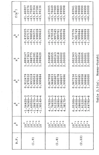
(ii) Rosen-Suzuki. (Rosen and Suzuki (1965)).

Minimize f (x) = x 2+ x i! + 2x"+x'-5x,-5x -21x + 7x

~ 1 2 3 * h 1 2 .5

subject to g (x)=-x^-x^-x'-x,+x -x^+x^+8 £ 0,

g 2 (x) =-xJ-2x^-x^-2x^+x. +X.+10 > 0,

g3(x)=-2xt“X^- x ^ - 2 x 4+x.+x.+5 > 0,

T

The constrained minimum is at x* = (0,1,2,-1) with

f(x*) = -44 and the first and third constraints active.

An initial feasible point is x u = (0,0,0,0)T with

f (x0) = 0 .

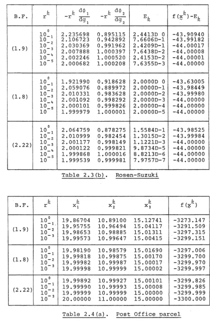
(iii) Post Office parcel p roblem. (Rosenbrock (1960)).

Minimize f(x) = -x x x

~ 1 2 3

subject to 0 $ x. < 20, 0 < x^ $ 11, 0 < x £ 42 and

0 £ x + 2x + 2x £ 7 2 .

1 2 3

T

The constrained minimum is at x* = (20,11,15) with

f(x*) = -3300 and the upper bounds on the first and

second variables as well as the last constraint active.

An initial point is x u = (15,3,25)T with f ( x J) = -1125.

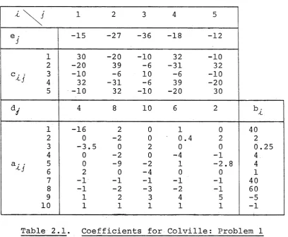
(iv) Colville: Problem 1. (Colville (1968)).

5 5 5 5

Minimize f (x) = 2 e x 3-1 j 1

+ Z

i= 1 r=l h cx./xx x /+ . k d ix )J J j=1 J J

5 subject to

= a i j

j=i j */

+ b - > 0 , i.=l, 10 ,

and

q l + 1 0 (x) = x^ > O r

L

T

)

i—

1

II

where a«;, c ■ ;, b*, d*, e ; are given in Table 2.1.

48

-3.5 0.25

- 2.8

Table 2.1. Coefficients for Colville: Problem 1

The constrained minimum is at x* = (0.3,0.3334676,0.4,

0.4283101,0.2239649)T with f(x*) = -32.34868 and the

third, fifth, sixth and ninth constraints active.

An initial feasible ooint is x u = (0.125,0.0625,0.125,

0.125,1.0)T with f (x 0 ) = 4.724609 .

Each problem has been solved using the three

barrier function transformations (1.8), (1.9) and

h h 1

T(x,r ) = f(x) + r £ log[10-log(g • (x))] .

i = i -t ~

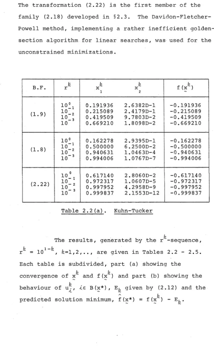
The transformation (2.22) is the first, member of the family (2.18) developed in §2.3. The Davidon-Fletcher- Powell method, implementing a rather inefficient golden-

section algorithm for linear searches, was used for the unconstrained minimizations.

B.F. r fz X fz Xfz

1 2

'

fz f ( X )

(1.9)

1 0 » i

1 0 — 2

1 0 - 3 10

0.191936 2.6382D-1 0.215089 2.4179D-1 0.419509 9.7 803D-2 0.669210 1.8098D-2

-0.191936 -0.215089 -0.419509 -0.669210

( 1 . 8 )

1 0 ° 10 1 10 2 1 0 ' 3

0.162278 2.9395D-1 0.500000 6.2500D-2 0.940631 1.0463D-4 0.994006 1.0767D-7

-0.162278 -0.500000 -0.940631 -0.994006

(2.22)

1 0 - , 1 0 - 2 10

10-3

0.617140 2.8060D-2 0.972317 1.0607D-5 0.997952 4.2 958D-9 0.999837 2.155 3D-12

-0.617140 -0.972317 -0.997952 -0.999837

Table 2.2(a). Kuhn-Tucker

The results, generated by the r -sequence, r^ = 101 k, fc=l,2,.., are given in Tables 2.2 - 2.5. Each table is subdivided, part (a) showing the

fz fz

convergence of x and f (x ) and part (b) showing the

fz

behaviour of u^, te B(x*), given by (2.12) and the

~ fz