Configuration of a smectic A liquid crystal due to an isolated edge dislocation

Configuration of a Smectic A Liquid Crystal Due to an Isolated Edge

Dislocation

B. C. Snow

Department of Mathematics, University of York, Heslington, York, YO10 5DD

I. W. Stewart

School of Science & Engineering, Fulton Building, University of Dundee,

Dundee, DD1 4HN

Wednesday 15

_{March, 2017}

Abstract

We discuss the static configuration of a smectic A liquid crystal subject to an edge dislocation under the assumption that the director and layer normal fields (n_anda_{, respectively) defining the smectic arrangement are}

not, in general, equivalent. After constructing the free energy for the smectic, we obtain exact solutions to the equilibrium equations which result from its minimisation at quadratic order in the variables which describe the distortion, and hence a complete description of the smectic configuration across the domain of the sample. We also examine the effect of relaxing the constraintn_≡a_{for different values of the constants which characterise}

the response of the material to distortions, and compare these results with the “classical” case considered by previous authors, in which equivalence ofn_anda_{is enforced.}

1

Smectic A Liquid Crystals

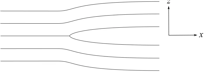
Liquid crystals (LCs) are mesomorphic phases of matter which are exhibited by materials consisting of anisotropic rod- or disc-like molecules. The LCs exist in temperature ranges between those of the material’s isotropic liquid and crystalline solid phases, and display physical properties reminiscent of both. General information on the physical properties of various LCs may be found, for instance, in the book of de Gennes and Prost [9]; more mathematical introductions are to be found in the works of Stewart [20] and Virga [24]. We will be concerned with the smectic A (SmA) phase [21], in which the constituent rod-like molecules align themselves along an axis of anisotropy, as found in the well-studied nematic phase, in addition to arranging themselves into layers such that, in an unstrained configuration, the anisotropic axis lies perpendicular to the local layer alignment; see Fig. 1(a). As such, it proves convenient to describe SmA by means of two unit vectors: the director,n_{, defining}

the local molecular orientation, and the unit layer normal,a_{, which describes the local layer structure.}

n₌a

(a)Relaxed planar configuration of SmA. _{(b)Distorted configuration induced by an applied} stress.

Figure 1: (a)In the absence of external stresses, a SmA sample with no defects will tend to align in a relaxed configuration such thatn_≡a_{. (b)Applying a stress leads to a distortion in which}n_anda_{may separate.}

Motivated by the observations of Auernhammeret al.[1–3], Elston [7], and Soddemannet al.[19], we allow for the possibility thatn_anda_{may separate under the imposed distortion, as depicted in Fig. 1(b). We assume}

that the free energy associated with any departure of the SmA from its unstrained configuration is of the form set forth by De Vita & Stewart [6]:

wDS=1₂K

a

1(∇ ·a)2+12K

n

1(∇ ·n−s0)2+12K2∇ · {(n· ∇)n−(∇ ·n)n}

+1 2B0|∇Φ|

−2

(1− |∇Φ|)2+1₂B1

1−(n_·a₎2 _{+B2(∇ ·}n_{) 1− |∇Φ|}−1

, (1.1)

where the scalar function Φ defines the layer normala_via a₌ ∇Φ

|∇Φ|. (1.2)

In equation (1.1),Ka

1,K1n, andK2 are elastic constants andB0,B1, andB2 are constant energy densities. The

first term on the right-hand side is the energy associated with bending of the smectic layers; the second term is the splay energy, withs0denoting the spontaneous splay; the third term is the saddle-splay energy; the fourth is the energy associated with layer compression/expansion; the fifth is the energy attributed to coupling between

n _anda_{; the sixth and final term is the energy due to coupling between splay and compression of the layers.}

Equation (1.1) provides a general description of the energy associated with deformations of a lipid bilayer. Note that we will be concerned only with SmA LCs with no polarisability or spontaneous splay, and thus the free energy we require is given by [6]

wA= 1₂K

a

1(∇ ·a)2+12K

n

1(∇ ·n)2+12K2∇ · {(n· ∇)n−(∇ ·n)n}

+1 2B0|∇Φ|

−2₍₁

− |∇Φ|)2+1 2B1

1−(n_·a₎2 _{. (1.3)}

A comprehensive account of the manner in which Φ defines the layer structure, as well as the physical properties of the energy in equation (1.1) and a range of applications to problems concerning the behaviour of lipid bilayers, may be found in the paper of De Vita and Stewart [6].

Background material on the theory of edge dislocations in crystalline solid media may be found in refer-ences [10, 12, 13]; for information regarding dislocations in smectics, the reader may consult the latter two of these references or the book of de Gennes and Prost [9, Section 9.2].

The article is organised as follows. In Section 2, we present the free energy at quadratic order in the director deflection and layer displacement, from which we derive the equilibrium equations and obtain an exact solution for the latter at that order. The derivation of the free energy, which we have constructed to fourth order, is deferred until Appendix A since the resulting expressions are unwieldy; in addition to enabling the computation of the results contained in the main body of the paper, this allows us to recover a known higher-order solution, details of which are presented in Appendix B. In Section 3, the solution for the layer displacement at quadratic order is compared graphically with the “classical” two-constant case, in which the director and layer normal are constrained to be identical throughout the sample, by means of rewriting both solutions as suitable integrals over a finite domain and numerically integrating the resultant expressions. In Section 4, we use the results obtained to arrive at expressions for both the director profile and the layer normal, thus providing a complete description of the static configuration of the SmA in the presence of the dislocation. Section 5 closes with a summary of the results obtained and suggestions for further work.

2

Separation of Director and Layer Normal at Quadratic Order

z

x

Consider a sample of SmA subject to an edge dislocation such that the Burgers vector of the dislocation [9, Section 9.2], which will be taken to have magnitudeb=d, withddenoting the interlayer spacing of the SmA, is parallel to thez-axis; the dislocation axis is parallel to they-axis. We wish to measure the deviation of the configuration of the SmA away from that of the reference configuration, described by

n₌n_{0≡(0,0,1), Φ = Φ0≡z. (2.1)}

The imposed dislocation will lead to a director profile of the general form

n_{= (sinθ(x, z), 0, cosθ(x, z)), (2.2)}

while the function Φ is modified to read

Φ =z−u(x, z). (2.3) From the latter of these equations, it readily follows that∇Φ = (−ux, 0, 1−uz), and thus

a_{= √}(−ux, 0, 1−uz)

1−2uz+u2x+u2z

, (2.4)

where, for ease of notation, we employ the convention that a variable appearing as a subscript denotes partial differentiation with respect to that variable. Given the somewhat unwieldy form of equation (2.4), it makes sense to follow previous work [4, 13] and anticipate only small deviations away from the reference configuration, and that such deformations occur over distances such that we need only take into account terms to quadratic order in a Taylor series of the pertinent variables when computing the free energy.

A derivation of the free energy to quartic order is contained in Appendix A. In spite of the lengthiness of some of the resultant expressions, all results in aforementioned previous works are readily obtained by truncation at the appropriate lower order.

2.1

Equilibrium Equations

We depart from the precedent set forth in previous work and allow n _and a _{to separate. By only retaining}

quadratic terms inu,θ, and their spatial derivatives, we obtain analytical expressions, exact up to this order of approximation, for both uandθ. According to equation (A.14), the free energywA may be written to second

order as

wA= 1₂

K1au2xx+K1nθ2x+B0u2z+B1(θ+ux)2 . (2.5)

We seek minimisersuandθof the total energy per unit length iny, given by

W =

Z

D

wAdA, (2.6)

where Ddenotes the two-dimensional domain occupied by the SmA sample; hereD=R2. We require the first variation of the total energy, δW, to be zero. It is readily shown [5] that this requirement is expressed by the following two PDEs:

∂2 ∂x2

_∂w

A

∂uxx

= ∂

∂x

_∂w

A

∂ux

+ ∂

∂z

_∂w

A

∂uz

, (2.7)

∂ ∂x

∂wA

∂θx

= ∂wA

∂θ . (2.8)

Carrying out the required partial differentiation shows that these are equivalent to

K1auxxxx=B0uzz+B1(θx+uxx), (2.9)

K1nθxx=B1(θ+ux), (2.10)

respectively. Note that requiringn₌a_{to second order givesθ+ux= 0, allowing for the recovery of the classical}

case; we proceed with the general casen₆₌a_.

The boundary conditions imposed are motivated by the anticipated dislocation structure. Choosing the origin (x, z) = (0,0) of our coordinate frame to lie at the core of the dislocation, we will solve the equations (2.9) and (2.10) in the half-spacez >0; we require (see Fig. 2)

u(x,0) = b

4(1 + sgn(x)), sgn(x) =

(

−1 x <0,

1 x >0. (2.11)

Further, we assume the distortion tends to zero in the far-field, so that

ux(x, z)→0, uz(x, z)→0, θ(x, z)→0 as|x| → ∞ for allz >0, (2.12)

and that the distortions are finite for allz in the upper half-plane:

2.2

Solution for the Layer Displacement

Differentiating (2.9) twice with respect toxand rearranging gives

θxxx=

Ka

1

B1uxxxxxx− B0

B1uzzxx−uxxxx,

so that, on substitution into the derivative of (2.10) with respect tox, it follows that

B1(θx+uxx) =K1n

Ka

1

B1uxxxxxx− B0

B1uzzxx−uxxxx

.

This may then be substituted into (2.9) to yield

λ2n uzzxx−λ2auxxxxxx+β λ2a+λ2n

uxxxx−uzz = 0, (2.14)

where we have introduced the length scales

λa=

p

Ka

1/B0, λn=

p

Kn

1/B0, (2.15)

in order to facilitate later comparison with previously-established results, along with the dimensionless parameter

β, given by

β=B1/B0. (2.16) We note here that, based on the work of Ribotta and Durand [16], we anticipate on physical grounds thatβ.1 for any given sample of SmA. Nevertheless, we will have cause to refer to the limit as β→ ∞in what follows; we stress that this limit is unphysical and purely for mathematical convenience and the elucidation of features of the more general free energies in equations (1.1) and (1.3).

Following the observation by Kleman and Lavrentovich [12] for the classical case, let us assume that the general solution to the PDE (2.14) in the regionz >0 may be expressed in the form

u(x, z) = b 4

1 +1

π

Z ∞

−∞

g(z)eiσx

iσ dσ

. (2.17)

Substitution into (2.14) readily yields the following ODE for g(z) in terms of the combination of parameters Γ(σ):

g′′(z) =σ

4

λ2

aλ2nσ2+β λ2a+λ2n

λ2

nσ2+β

g(z)≡Γ2(σ)g(z), (2.18)

whose general solution is

g(z) =A(σ)e−Γ(σ)z+B(σ)eΓ(σ)z.

Based on (2.13)1, we requireg(z) to be finite for allz >0, and so it immediately follows thatB(σ) = 0. Further,

the boundary condition (2.11) leads to the requirement

Z ∞

−∞

A(σ)eiσx

iσ dσ=πsgn(x). (2.19)

Now, it may readily be shown by expanding eiσx = cos(σx) +isin(σx), substitutingσx →τ and integrating along an appropriate contour in the complex plane that

Z ∞

−∞ eiσx

iσ dσ= 2 sgn(x)

Z ∞

0

sinτ

τ dτ =πsgn(x),

from which it is evident that we may chooseA(σ)≡1, and thus

u(x, z) = b 4

1 +1

π

Z ∞

−∞

eiσx−Γ(σ)z

iσ dσ

= b 4+

b

2π

Z ∞

0

e−Γ(σ)zsin(σx)

σ dσ. (2.20)

3

Comparison with the Two-Constant Case

Let us denote the layer displacement in the classical case byυ(x, z). This may be written in the form [12]

υ(x, z) = b 4 1 +

1

π

Z ∞

−∞

eiσx−λσ2_z

iσ dσ

!

=b 4+

b

2π

Z ∞

0

e−λσ2_z

sin(σx)

σ dσ, (3.1)

where λ2 =λ2a+λ2n. To facilitate graphical comparison of this displacement with that given above by

equa-tion (2.20), it proves convenient to write each of the expressionsυanduabove in terms of integrals over a finite domain. This is achieved by appeal to the substitution

ζ= 1

1 +λσ =⇒ dσ=− dζ

λζ2, (3.2)

so that equation (2.20) may, after appropriate substitution and rearrangement, be written in the form

u(x, z) = b 4+

b

2π

Z 1

0

f(ζ)dζ, (3.3)

where

f(ζ) = exp{−∆(ζ)z}sin

ζ−1₋₁

x/λ

ζ−ζ2 , (3.4)

with

∆(ζ) = (1−ζ)

2

λ2

s

λ2

aλ2n(ζ−1−1)2+βλ4

λ2

n(ζ−ζ2)2+βλ2ζ4

. (3.5)

One readily deduces that

∆(ζ)→ ∞ as ζ→0+, ∆(ζ)→0 as ζ→1−,

from which

f(ζ)→0 as ζ→0+, f(ζ)→ x_λ as ζ→1−_{, (3.6)}

which ensure that the integral does not diverge. Utilising (3.2) in (3.1) yields

υ(x, z) = b 4+

b

2π

Z 1

0

k(ζ)dζ, (3.7)

where

k(ζ) =

expn− ζ−1−12

z/λosin

ζ−1−1

x/λ

ζ−ζ2 , (3.8)

which is readily obtained as f(ζ) in the (unphysical) limit as β → ∞. It is therefore evident that the two displacements agree at the endpoints of integration by virtue of the limits offin equation (3.6) being independent ofβ. We note that the diffusion-like property of the spatial derivatives ofυ

∂zυ=λ∂x2υ, (3.9)

does not hold foru; instead, we have the relationship

λ∂x2u−∂zu= b

2π

Z ∞

0

Γ(σ)

σ −λσ

e−Γ(σ)zsin(σx)dσ. (3.10)

The properties stated in equations (3.6) allow for numerical integration of the expressions forυanduoutlined in equations (3.3)–(3.5) and (3.7), (3.8), respectively, by defining the function f(ζ) in a piecewise manner over the interval [0,1] and appealing to theApproximateInt command in Maple [14]. From this, a range of plots has been generated for typical SmA parameter values [22].

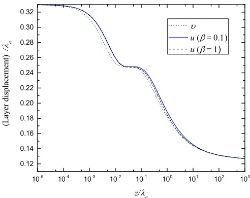
Displayed in Figs. 3(a),(b) below, we see the displacementsuandυdue to the dislocation plotted as functions of z, selectingβ = 0.1 andβ = 1 for the former. Also shown is the difference between the two quantities for these values ofβ. Note that we have setx=λa =λn, and the valueb=λa/2 has been chosen to ensure the

the dislocation in the classical case and β= 0.1, with similar non-negligible differences found when comparing the classical solution with the caseβ= 1.

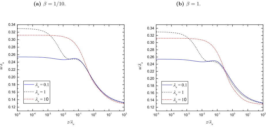
Next, Figs. 4(a), (b) show the effects of varying the constantK1nin the casex=λaas before; plots are shown

forλn=λa/10,λa, and 10λawith values ofβas indicated in the relevant captions. This variation has an even

more pronounced influence on the predicted values ofu, particularly forz close to the core of the dislocation. It follows from the results presented here that the more general free energy proposed by De Vita and Stewart constitutes a significantly refined model for the energetics of SmA, furnishing us with predictions for a wider range of SmA samples in which the experimentally observed phenomenon of director/layer normal decoupling is non-negligible.

Figure 3: Effect of variation ofβupon the layer displacement, plotted as a function ofz forx=λa=λn.

(a)The normalised layer displacements for values ofβwithin its physically allowable range.

10

-5

10

-4

10

-3

10

-2

10

-1

10

0

10

1

10

2

10

3

0.12 0.14 0.16 0.18 0.20 0.22 0.24 0.26 0.28 0.30 0.32

(

L

a

y

e

r

d

i

s

p

l

a

c

e

m

e

n

t

)

/

a

z/

a

u ( = 0.1 ) u ( = 1 )

(b) The difference between the solutionuas seen in equation (2.20) and the classical solutionυstated in equation (3.1).

10

-5

10

-4

10

-3

10

-2

10

-1

10

0

10

1

10

2

10

3

-0.002 0.000 0.002 0.004 0.006 0.008 0.010 0.012

(

u

-)

/

a

z/

a

Figure 4: The normalised layer displacements for various values of the parametersλnandβ.

(a)β= 1/10.

10 -5 10 -4 10 -3 10 -2 10 -1 10 0 10 1 10 2 0.12 0.14 0.16 0.18 0.20 0.22 0.24 0.26 0.28 0.30 0.32 0.34 u / a z/ a n = 0.1 n = 1 n

= 1 0

(b) β= 1.

10 -5 10 -4 10 -3 10 -2 10 -1 10 0 10 1 10 2 0.12 0.14 0.16 0.18 0.20 0.22 0.24 0.26 0.28 0.30 0.32 0.34 u / a z/ a n = 0.1 n = 1 n

= 1 0

4

Solutions for Director Profile and Layer Normal

It still remains for us to derive an expression forθ. To this end, equation (2.9) is easily rearranged to yield

θx=

λ2

a

β uxxxx−

1

βuzz−uxx. (4.1)

Carrying out the required differentiation leads to

θx=

b 2π Z ∞ 0 λ2

aσ3

β +σ−

Γ2_(σ) βσ

e−Γ(σ)zsin(σx)dσ. (4.2)

Integration of equation (4.2) with respect toxgives the general solution

θ= b 2π

Z ∞

0

χ(σ){cos(σx) +τ(z)}dσ, (4.3)

where

χ(σ) =

_Γ2_(σ)

βσ2 − λ2

aσ2

β −1

e−Γ(σ)z, (4.4)

andτ(z) is an arbitrary function ofzarising from the integration. On physical grounds, we must haveθ(x, z)→0 as |x| → ∞ ∀z >0, as per (2.12)3; then, sinceχ(σ) has only a finite number of maxima and minima and no

discontinuities forσ∈[0,∞), we may utilise [18, Section 3, Theorem 4] to determine that

lim

x→∞θ(x, z) = b 2 lim x→∞ Z ∞ 0

χ(σ) cos(σx)dσ+ lim

x→∞

Z ∞

0

χ(σ)τ(z)dσ

=⇒

Z ∞

0

χ(σ)τ(z)dσ= 0. (4.5)

Hence, rewriting Γ2_{(σ) in the form}

Γ2(σ) =λ2aσ4

1 + βλ

2

n

λ2

a(λ2nσ2+β)

,

we readily arrive at

θ(x, z) = b 2π

Z∞

0

χ(σ) cos(σx)dσ= b 2π

Z ∞

0

λ2

nσ2

λ2

nσ2+β−

1

e−Γ(σ)zcos(σx)dσ. (4.6)

Note that, in the limit asβ→0, it is straightforward to deduce

lim

β→0χ(σ) = (1−1)e −λaσ

2

z_{= 0 =}

⇒ lim

β→0θ(x, z) = 0, (4.7)

and hence β = 0 corresponds to no director distortion. Based on our definition ofβ in equation (2.16), it is straightforward to see that this is the limit in which there is no energetic cost associated with separation between

n_anda_{. It follows that any layer compression in this limit must be negligible, so that the constituent molecules}

may remain aligned along the z-axis as in the relaxed configuration. (Note that this does not rule out layer expansion, however.)

Rewriting Γ2_{(σ) in the form}

Γ2(σ) =λ2σ4

1 + (λ2aλ2nσ2/βλ2)

1 + (λ2

nσ2/β)

and continuing to increaseβleads to

lim

β→∞Γ

2_{(σ) =λ}2_σ4_{, lim}

β→∞χ(σ) =−e −λσ2_z

, (4.8)

and thus

lim

β→∞θ=−βlim→∞ux=− b

2π

Z ∞

0

e−λ2σzcos(σx)dσ, (4.9)

appearing to recover the result of the classical case n₌a_{; see equations (3.9), (3.10). However, as noted in}

Section 2.2 after equation (2.16), this corresponds to a purely formal limit with no physical relevance since

β.1 [16], and hence the classical solution cannot be derived from the more general case for physically realisable values of the parameters characterising the SmA. Since the results for the classical case show significant deviation from those arising from (2.20), we propose that the more general free energy presented in Section 1 is more suitable for modelling the energetics of static phenomena in SmA samples where the difference between director and layer normal is significant.

Following the approach of the preceding section, let us write the expression (4.6) as an integral over the finite interval [0,1]. Employing the substitution (3.2) once more, it follows thatθ may be expressed in the equivalent form

θ(x, z) = b 2πλ

Z 1

0

h(ζ)dζ, (4.10)

where

h(ζ) =

λ2n(ζ−1−1)2

λ2

n(1−ζ)2+βλ2 −

1

ζ2

e−∆(ζ)zcos

ζ−1−1

x/λ . (4.11)

It is readily deduced that, asζ→0+_,

|h(ζ)|=O

1

ζ4e −1/ζ3

,

and thus

h(ζ)→0 asζ→0+, h(ζ)→ −1 asζ→1−, (4.12) from which it is evident that the integral will not diverge. Letδbe the angle betweena_{and the positivez-axis;}

the layer normal may be expressed in the form

a_{= (sinδ,0,cosδ)≈ −ux(1 +uz),0,1 +uz+u}2_z−1

2u 2

x

,

from which it is evident that, to quadratic order,

δ= arcsin{−ux(1 +uz)}. (4.13)

Recalling equation (3.3), it is straightforward to conclude that

ux= b

2πλ

Z 1

0

µ(ζ)dζ, (4.14)

uz=

b

2π

Z 1

0

ν(ζ)dζ, (4.15)

where we have defined

µ(ζ) = e

−∆(ζ)z_cos

ζ−1₋₁

x/λ

ζ2 , (4.16)

ν(ζ) = ∆(ζ)e

−∆(ζ)z_sin

ζ−1₋₁

x/λ

We record that

µ(ζ)→0 asζ→0+, µ(ζ)→1 asζ→1−, (4.18)

ν(ζ)→0 asζ→0+, ν(ζ)→0 asζ→1−. (4.19) Taken together, the expressions obtained foru in (3.3)–(3.5) and forθ in (4.10), (4.11) allow us to determine expressions for the directorn _{and the layer normal}a_{, and hence the alignment of the SmA, across the entire}

sample to quadratic order in the variables characterising the distortions induced by the edge dislocation.

5

Conclusions and Discussion

This article has examined the effects of an isolated edge dislocation on the static configuration of a SmA liquid crystal. After deriving the relevant expression for the total SmA free energy and the resulting equilibrium equations that must be satisfied by the director deflection and layer displacement, it was shown that, in the absence of the constraint that n_{must always coincide with} a_{, it is possible to construct exact solutions for}

both the layer displacement and director deflection when the free energy is truncated at quadratic order. These expressions provide us with a complete description of the SmA sample in the presence of this dislocation in terms of its departure from the relaxed configuration of planar layers with n _≡a_{. Moreover, the solution u}

for the layer displacement differs substantially from the classical case in whichn_anda_{always coincide, as was}

demonstrated by the modified identity expressed in equation (3.10), as well as the plots contained in Figs. 3–4 for various values of the relevant elasticity and energy terms.

The differences between the predictions of the more general framework of De Vita and Stewart and those of the classical case justify the use of the former as a model for SmA samples in which this separation plays a non-negligible role in determining their behaviour in equilibrium settings such as that considered here and when undergoing motion (see, for instance, reference [23]). Given that significant decoupling between n_and a _has

been demonstrated in previous work [1–3, 7, 19], it is clear that such a model provides valuable insight which is surely necessary for those wishing to fully understand the rich and complex behaviour of the SmA phase.

Many further avenues of investigation present themselves. Having explored the isolated edge dislocation case, it may be of interest to investigate configurations of multiple dislocations and ask what sort of distortion is to be anticipated, as well as how different strengths and configurations of these defects would alter the smectic structure. It might also prove pertinent to examine the dynamics to which this would lead or, conversely, how the imposition of flow (for example by the application of a pressure gradient across the sample) might affect the configurations considered here.

Screw dislocations [9, Subsection 9.2.1.3] may be investigated along similar lines and these remain to be analysed in the context of the theory presented above; the interplay between layering structure and a more flexible director orientation relative to the layers may well lead to a more refined description and model for such structures. A consequent energy analysis may also provide fresh insight to the smectic layer structure close to the defect points.

Finally, it has been assumed throughout that the sample under consideration has infinite spatial extent: physically speaking, this corresponds to assuming that the sample boundaries are sufficiently far from the core of the defect so as to have no effect on the resultant configuration. It may prove worthwhile to examine the case of a dislocation near to a boundary under a variety of anchoring conditions. Such matters certainly warrant a great deal of further exploration.

A

Calculating the Free Energy to Fourth Order

Equation (2.2) may be approximated by

n_{= θ−}1

6θ 3_{, 0, 1}

−1 2θ

2₊ 1 24θ

4

, (A.1)

from which it is readily deduced thatn_·n_{= 1 +O(θ}6_{). Further, on noting that, forv≪1}

√

1 +v= 1 +1 2v−

1 8v

2₊ 1

16v

3

−₁₂₈5 v4+O(v5),

1

√

1 +v = 1−

1 2v+

3 8v

2

− 5

16v

3₊ 35

128v

4₊

O(v5),

it is easy to show that the approximations

|∇Φ|= 1−uz+1₂u2x+12u 2

xuz−1₈u4x+12u 2

xu2z, (A.2)

|∇Φ|−1= 1 +uz−1₂ux2+u2z+u3z−32u 2

hold to fourth order, and thus we may approximatea_as a_{= −ux−uxuz+}1

2u 3

x−uxu2z(1 +uz) +3₂u3xuz, 0, 1−1₂u2x−u2xuz+3₈u4x−32u 2

xu2z

. (A.4)

It readily follows thata_{is also a unit vector to fourth order. We may now use equations (A.1)–(A.4) to compute}

the terms comprisingwDS. Firstly, a simple calculation yields

(∇ ·a₎2_=u2_{xx+ 2u}2_{xxuz+ 4uxuxxuxz+ 3u}2_xxu2_{z+ 4u}2_xu2_xz−3u2_xu2_{xx+ 2ux}2_{uxxuzz+ 12uxuxxuzuxz, (A.5)}

while

(∇ ·n_−s0)2_=θ2_{x−2θθxθz+θ}2_(θ2_z−θ2_{x) +s0 s0−2θx+ 2θθz+θ}2_θz−1

3θ 3_θ

z

. (A.6)

Tedious but straightforward calculations allow us to conclude that

(n_{· ∇)}n_{−(∇ ·}n₎n_{= (θz,0,−θx), =⇒ ∇ · {(}n_{· ∇)}n_{−(∇ ·}n₎n_{}= 0, (A.7)}

where it is assumed that partial derivatives ofθcommute. Squaring both sides of equation (A.3) leads to

|∇Φ|−2= 1 + 2uz−u2x+ 3u2z+ 4u3z−4u2xuz+u4x+ 5uz4−10u2xu2z, (A.8)

which, taken in conjunction with (A.2), allows us to conclude

|∇Φ|−2(1− |∇Φ|)2=u2z+ 2u3z−u2xuz+1₄u4x+ 3uz4−4u2xu2z. (A.9)

Equations (A.1) and (A.4) may be combined to yield

n_·a_{= 1−θux−}1

2θ 2

−u2xuz+1₂θux3−θuxu2z+16θ 3_u

x+3₈u4x−32u 2

xu2z+241θ 4₊1

4θ 2_u2

x, (A.10)

from which

1−(n_·a₎2_=θ2_+u2_{x+ 2θux+ 2u}2_{xuz+ 2θuxuz−}1

3θ 4

−u4x−2θu3x

−4 3θ

3_u

x−2θ2u2x+ 2θuxu2z+ 3u2xu2z. (A.11)

Finally, since

∇ ·n_{=θx−θθz−}1

2θ 2_θ

x−1₆θ3θz, (A.12)

it may be deduced by further appeal to equation (A.3) that

(∇ ·n_{) 1− |∇Φ|}−1

=−θxuz+1₂θxu2x−θxu2z+θθzuz−θxu3z

+3 2θxu

2

xuz−1₂θθzu2x+θθzu2z+1₂θ2θxuz. (A.13)

Putting all this together, the free energywDS may be expressed to fourth order in the form

wDS=1₂K1a(uxx2 + 2u2xxuz+ 4uxuxxuxz+ 3u2xxu2z+ 4ux2u2xz−3u2xu2xx

+ 2u2xuxxuzz+ 12uxuxxuzuxz) +1₂K1n

θ2x−2θθxθz+θ2(θz2−θx2)

+s0 s0−2θx+ 2θθz+θ2θz−1₃θ3θz +1₂B0 u2z+ 2u3z−u2xuz+1₄u4x

+ 3u4z−4u2xu2z

+1 2B1 θ

2_+u2

x+ 2θux+ 2u2xuz+ 2θuxuz−1₃θ4−u4x

−2θu3x− 43θ 3_u

x−2θ2u2x+ 2θuxu2z+ 3u2xu2z

+B2 −θxuz+1₂θxu2x

−θxu2z+θθzuz−θxu3z+ 32θxu 2

xuz−1₂θθzux2+θθzu2z+12θ 2_θ

xuz. (A.14)

As stated in Section 1, the free energywAfor samples of SmA consisting of non-polarisable molecules is recovered

whens0=K2=B0= 0.

B

Director and Layer Normal Coincident: Recovering the Brener

and Marchenko Solution

In the case wheren_≡a_{, the free energy simplifies to read}

wA= 1₂(K₁a+K₁n)(∇ ·a)2+1₂B0|∇Φ|−2(1− ∇|Φ|)2

≡ 1

whereK1=Ka

1 +K1n, and w0= uz−1₂u2x

2

+u3z(2 + 3uz)−4u2xu2z, (B.2)

w1=u2xx+ 2u2xxuz+ 4uxuxxuxz+ 3u2xxu2z+ 4u2xu2xz−3u2xu2xx+ 2u2xuxxuzz+ 12uxuxxuzuxz. (B.3)

Let us calculate the first variation of the energyδW, defined for admissible variationsh[8, 17] by

δW = d

dt

Z Z

R2

η dxdz

t=0

=

Z Z

R2{

∂t(η0+η1)}|t=0 dxdz, (B.4)

where

η0 =w0(u+th)−w0(u), η1 =w1(u+th)−w1(u), (B.5)

and

η=η0+η1=wA(u+th)−wA(u). (B.6)

It is a tedious but simple matter to compute the following:

η0 =t

hx(u3x−2uxuz−8uxu2z) +hz(2uz+ 6u2z−u2x+ 12u3z−8u2xuz) +O(t2), (B.7)

η1 =t

hxx(2uxx+ 4uxxuz+ 4uxuxz+ 6uxxu2z−6u2xuxx+ 2u2xuzz+ 12uxuzuxz)

+hxz(4uxuxx+ 8u2xuxz+ 12uxuxxuz) + 2hzzu2xuxx

+hx(4uxxuxz+ 8uxu2xz−6uxu2xx+ 4uxuxxuzz+ 12uxxuzuxz)

+hz(2u2xx+ 6u2xxuz+ 12uzuxxuxz) +O(t2), (B.8)

from which it readily follows that the integrand ofδW is simply the sum of the terms enclosed in curly brackets within equations (B.7) and (B.8). WritingδW =δW0+δW1, where

δW0=1 2B0

Z Z

R2

(∂tη0)|_t=0dxdz, δW1=1

2K1

Z Z

R2

(∂tη1)|_t=0dxdz,

it follows that we may, on integrating by parts and requiring that any admissiblehand spatial derivatives thereof vanish at the limits of integration, rewriteδW0 andδW1 in the respective forms

δW0=B0

Z Z

R2

h

uxx 4u2z−32u 2

x+uz

+uzz(4u2x−18u2z−6uz−1) + 2uxuxz(8uz+ 1) dxdz, (B.9)

δW1=K1

Z Z

R2

h

uxxxx(3u2z−3u2x+ 2uz+ 1) + 4uxuxxxz(3uz+ 1) + 6u2xuxxzz

+ 6uxxx(3uzuxz−2uxuxx+uxuzz+uxz) + 6uxxz(3uxxuz+ 5uxuxz+uxx)

+ 12uxuxxuxzz+ 3uxx(uxxuzz−u2xx+ 6u2xz) dxdz. (B.10)

The energyW is then minimised by settingδW =δW0+δW1 = 0 for all admissible variationsh, which yields a nonlinear and highly intractable partial differential equation foru. Progress regarding solutionsuto the full equation is probably best achieved by appeal to computational means, and this will not be considered here. However, assuming small layer displacements with sufficiently small spatial derivatives, analytical progress can be made in the following manner: according to both theoretical studies [9, Subsection 9.2.1] and experimental observations [11], the distortion of the layered structure is essentially confined to parabolic regions described by

x2_{=cλzfor some constantc, whereλ=}p

K1/B0, which tells us that this configuration relaxes back to planar layers rapidly alongxbut significantly less so alongz. Thus, if one assumes thatux∼u/ξanduz∼u/Lfor some

characteristic length scalesξ and L of displacement in thexand z directions, respectively, withξ2 _=O(λL),

it is apparent from equations (B.9) and (B.10) that, on regarding terms of magnitude smaller than ∼1/ξ4 as negligible, one immediately arrives at the truncated equilibrium equation

λ2uxxxx+uxx uz−3₂u2x

−uzz+ 2uxuxz= 0 (B.11)

for the casez >0; a similar equation is obtained in the casez <0. This is exactly the PDE obtained by Brener and Marchenko [4, equation (4)], which may be non-dimensionalised by means of measuring all lengths in terms ofλ; the non-dimensional form reads

uxxxx+uxx uz−3₂u2x

−uzz+ 2uxuxz= 0. (B.12)

It is readily checked via differentiation that a solutionu(x, z) of the equation

uxx=asgn(z) 2uz±u2x

also solves the equation

uxxxx= 4a2 uzz±uxxuz±2uxuxz+3₂u2xuxx, (B.14)

whereais some real number. (The casea= 1/2 with the lower signs chosen corresponds to equation (B.12); the casea= 1 with the upper signs chosen is the case considered by Nepomnyashchy and Pismen [15] for pattern-forming systems.) Further, if one introduces the similarity variablev=x/√z, the PDE (B.13) may be rewritten in the form

u′′=asgn(z)

±(u′)2−vu′ , (B.15) where ′

≡d/dv. To simplify notation, we will provide the general solution only for the casez > 0. To solve equation (B.15), introduce the transformation

u′=γ(v)e−av2/2.

We may then express the ODE (B.15) in the form

dγ dv =±aγ

2_e−av2/2_{, (B.16)}

a first-order separable ODE which may be integrated with respect tovto yield

−γ=

c1±a

Z v

−∞

e−at2/2dt

−1

, (B.17)

wherec1 is a constant of integration. The general solution foruis therefore

u(v) =∓_a1ln

∓a

Z v

−∞

e−at2/2dt−c1

+c2, (B.18)

where the constantsc1 and c2 are determined by appropriate boundary conditions onu. Thus, the solution to the PDE (B.12) may be deduced from this by settinga= 1/2, imposing the condition

lim

v→∞u(v)−v→−∞lim u(v) = b

2, applying the definition of the error function

erf(x) :=√2_π

Z x

0

e−t2dt,

and returning to dimensional variables to get

u= 2λln

1 2

1 +eb/4λ+ (eb/4λ−1) erf

x

2√λz

. (B.19)

It is straightforward to apply the same approach and thereby obtain the solution for z <0. Finally, we note that, in the limit whereb≪λ, one readily obtains

u∼2λln

1 + b 8λ

1 + erf

x

2√λz

∼₄b

1 + erf

x

2√λz

, (B.20)

which is equivalent to the result derived in the classical case [12, 13] as seen in equation (3.1).

Acknowledgements

References

[1] Auernhammer, G.K., Brand, H.R., Pleiner, H.: The undulation instability in layered systems under shear flow – a simple model. Rheol. Acta39, 215–222 (2000)

[2] Auernhammer, G.K., Brand, H.R., Pleiner, H.: Shear-induced instabilities in layered liquids. Phys. Rev. E

66, 061,707 (2002)

[3] Auernhammer, G.K., Brand, H.R., Pleiner, H.: Erratum: Shear-induced instabilities in layered liquids. Phys. Rev. E71, 049,901 (2005)

[4] Brener, E.A., Marchenko, V.I.: Nonlinear theory of dislocations in smectic crystals. Phys. Rev. E59, R4752 (1999)

[5] Courant, R., Hilbert, D.: Methods of Mathematical Physics, vol. 1. Wiley, New York (1989)

[6] De Vita, R., Stewart, I.W.: Energetics of lipid bilayers with applications to deformations induced by inclusions. Soft Matter9, 2056 – 2068 (2013)

[7] Elston, S.J.: The alignment of a liquid crystal in the smectic a phase in a high surface tilt cell. Liq. Cryst.

16, 151–157 (1994)

[8] Gel’fand, I.M., Fomin, S.V.: Calculus of Variations. Dover, New York (1991)

[9] de Gennes, P.G., Prost, J.: The Physics of Liquid Crystals, 2nd edn. Oxford University Press, Oxford (1993)

[10] Howell, P., Kozyreff, G., Ockendon, J.: Applied Solid Mechanics. Cambridge University Press, Cambridge, United Kingdom (2009)

[11] Ishikawa, T., Lavrentovich, O.D.: Dislocation profile in cholesteric finger texture. Phys. Rev. E60, R4752 (1999)

[12] Kleman, M., Lavrentovich, O.D.: Soft Matter Physics: An Introduction. Springer-Verlag, New York (2003) [13] Landau, L.D., Lifshitz, E.M.: Theory of Elasticity, Course of Theoretical Physics, vol. 7, 3rd edn.

Butterworth-Heinemann, Oxford (1984)

[14] Maplesoft: Maple 2015. Waterloo, Canada (2015)

[15] Nepomnyashchy, A.A., Pismen, L.M.: Singular solutions of the nonlinear phase equation in pattern-forming systems. Phys. Lett. A153, 427–430 (1991)

[16] Ribotta, R., Durand, G.: Mechanical instabilities of smectic A liquid crystals under dilative or compressive stresses. J. Physique38, 179–204 (1977)

[17] Sagan, H.: Introduction to the Calculus of Variations. Dover, New York (1992) [18] Sneddon, I.N.: Fourier Transforms. Dover, New York (2010)

[19] Soddemann, T., Auernhammer, G.K., Guo, H., D¨unweg, B., Kremer, K.: Shear-induced undulation of smectic a: Molecular dynamics simulations vs. analytical theory. Eur. Phys. J. E13, 141–151 (2004) [20] Stewart, I.W.: The Static and Dynamic Continuum Theory of Liquid Crystals. Taylor & Francis, London

(2004)

[21] Stewart, I.W.: Dynamic theory for smectic A liquid crystals. Continuum Mech. Thermodyn.18, 343–360 (2007)

[22] Stewart, I.W., Stewart, F.: Shear flow in smectic A liquid crystals. J. Phys.: Condens. Matter21, 465,101 (2009)

[23] Stewart, I.W., Vynnycki, M., McKee, S., Tom´e, M.F.: Boundary layers in pressure-driven flow in smectic A liquid crystals. SIAM J. Appl. Math.75, 1817–1851 (2015)