Rochester Institute of Technology
RIT Scholar Works
Theses Thesis/Dissertation Collections
8-19-2013
Optimization Modeling Approach to Facilitate
Decision Making Process of Energy Planning on
College Campuses
Sourabh Jain
Follow this and additional works at:http://scholarworks.rit.edu/theses
This Thesis is brought to you for free and open access by the Thesis/Dissertation Collections at RIT Scholar Works. It has been accepted for inclusion in Theses by an authorized administrator of RIT Scholar Works. For more information, please [email protected].
Recommended Citation
1
ROCHESTER INSTITUTE OF TECHNOLOGY
Optimization Modeling Approach to Facilitate Decision Making
Process of Energy Planning on College Campuses
by
Sourabh Jain
A Thesis Submitted in Partial Fulfillment of
Requirements for the Degree of Master of Science in Sustainable Engineering
Department of Industrial and Systems Engineering
College of Engineering
Rochester Institute of Technology
Rochester, NY
ii
DEPARTMENT OF INDUSTRIAL AND SYSTEMS ENGINEERING
KATE GLEASON COLLEGE OF ENGINEERING
ROCHESTER INSTITUTE OF TECHNOLOGY
ROCHESTER, NY
CERTIFICATE OF APPROVAL
---
M.S. DEGREE THESIS
---
The M.S. Degree thesis of Sourabh Jain
has been examined and approved by the
thesis committee as satisfactory for the
thesis requirements for the
Master of Science degree
Approved by:
--- Dr. Brian Thorn, Thesis Advisor
--- Dr. Ruben Proano, Co-Advisor
iii
Abstract
Increasing global environmental problems require a rapid response from universities (Sharp,
2002). Energy consumption of universities is increasing due to, for example, expansion in use of
electronics and new building constructions (Levine, 2009; Sharp, 2002). There are increasing
numbers of initiatives on university campuses to address climate change. The American College
and University President’s Climate Commitment (ACUPCC) is an effort by a group of colleges
and universities that have pledged to eliminate greenhouse gas (GHG) emissions from their
campus operations and become carbon neutral by a target date set by each university itself
(ACUPCC, 2006).
This research presented an optimization approach to help decision makers of universities find an
optimal energy plan that meet their environmental goals while minimizing costs associated with
those energy plans. The optimization approach takes into consideration annual energy demand,
budget constraints, and environmental constraints. This study analyzed the usefulness of a
long-term planning approach. The results showed that a single long-long-term energy plan was better than
integrated multiple short-term energy plans for a given planning horizon. However, long-term
energy plans required higher capital investments. In addition, Monte Carlo simulation is used to
analyze uncertainties associated with natural gas, electricity, and carbon prices. The optimization
approach developed in this work can be used by university decision makers to make long-term
iv
Acknowledgment
I would like to express my deepest appreciation to all those who helped me at least during the
past three years of my graduate studies. First, I would like to thank my parents (Deepchand and
Uma) for all of their sacrifices they made throughout their lives to send us to school and colleges.
They always motivated us to pursue our dreams.
I give a special gratitude to my main advisor, Dr. Brian Thorn, whose encouragement, support,
and feedback helped me to finish my thesis. Whenever I struggled with the thesis on any issue,
he always guided me in the right direction to reach my goal. I really appreciate support of my
other committee members. Dr. Ruben Proano helped me with the modeling part of my work. I
will always be grateful to him for letting me attend one of his courses on optimization. I would
also like to give special thanks to Dr. Robert Stevens. His suggestions help me turn my idea of
project into a research thesis.
I would also like to acknowledge with much appreciation the crucial role of financial support
provided by ISE department. Without this support, I would not have been able to attend the
gradual school.
I thank from bottom of my heart all my sustainable and unsustainable friends at RIT. I am
thankful to Christopher, Dmitry, and Jamie for introducing me with the American culture, which
was one of mine childhood dreams.
Last but not least, many thanks go to me, Sourabh Jain, who invested his full effort, energy, and
nine months of focused work to achieve this goal. I have to appreciate my perseverance of not
v
Dedicated to One of My Favorite Quotes:
vi
Table of Contents
Table of Contents ... vi
Chapter 1. Introduction ... 1
1.1 Motivation: ... 1
1.2 Problem Statement ... 5
Chapter 2. Literature Review ... 8
2.1 Mathematical Models in Energy Planning ... 8
Chapter 3. Methodology ... 13
3.1 Mathematical Programming ... 13
3.2 Model Formulation ... 14
3.2.1 Sets and Indices:... 15
3.2.2 Parameters: ... 16
3.2.3 Decision Variables: ... 18
3.2.4 Objective Function ... 18
3.2.5 Model Constraints ... 21
3.3 Monte Carlo Simulation (MCS) ... 25
Chapter 4. Experiment ... 28
4.1 Background Information on the Campus ... 29
4.2 Analysis Method... 31
vii
4.2.2 Uncertainty Analysis ... 34
4.3 Data for the Analysis ... 35
4.3.1 Different Planning Periods ... 35
4.3.2 Annual Investment Limits ... 35
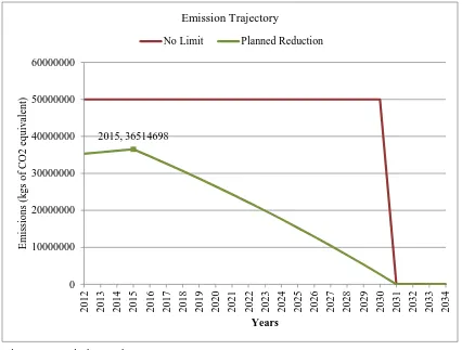
4.3.3 Different Emission Trajectories ... 36
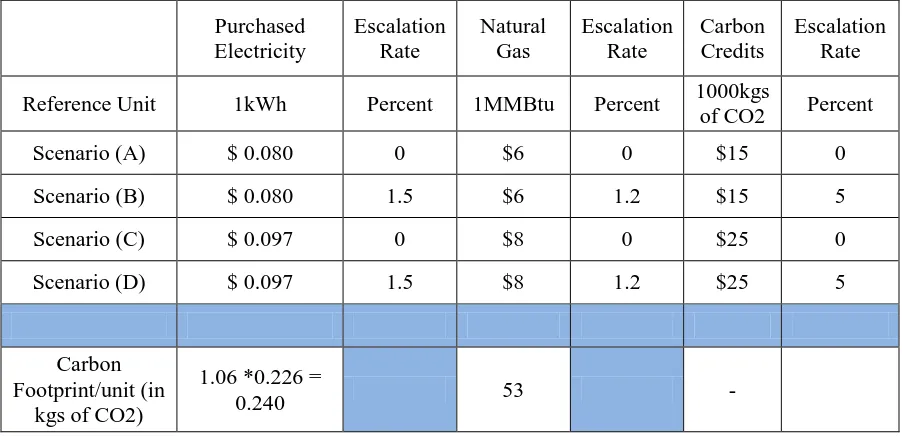
4.3.4 Energy and Carbon Prices for Various Scenarios ... 37
4.3.5 Uncertainty in Electricity, Natural gas, and Carbon prices ... 39
4.3.6 Energy System of the Campus ... 40
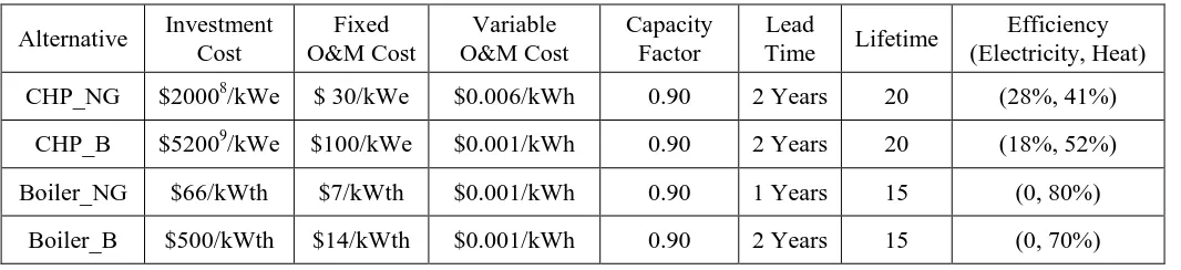
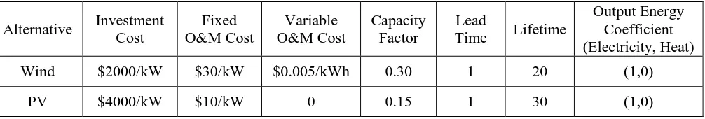
4.3.7 Cost and Technical Data of Energy Alternatives ... 44
4.3.8 Emission Data ... 46
4.3.9 Uncertainty in the Data ... 47
4.3.10 Energy Prices ... 47
4.3.11 Carbon Prices ... 47
Chapter 5. Results ... 50
5.1 Results and Analysis for the First Part ... 50
5.1.1 Short Term Planning vs. Long Term Planning ... 50
5.1.2 Effects Investment Constraints ... 55
5.1.3 Effects of Planned Emission Reduction ... 58
viii
5.2 Part II: Uncertainty Analysis ... 66
Chapter 6. Discussion and Conclusion ... 71
Chapter 7. Future Work ... 74
Chapter 8. Bibliography ... 76
ix
List of Figures
Figure 4-1 GHG Emission Pie Chart-2010 ... 30
Figure 4-2 Analysis Method ... 32
Figure 4-3 Emission Trajectory ... 36
Figure 4-4 Historical Energy Consumption ... 41
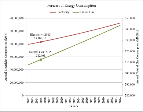
Figure 4-5 Forecast of Energy Consumption ... 43
Figure 5-1 Cost distribution of energy plan EP1 ... 68
Figure 5-2 Cost distribution of energy plan EP2 ... 68
x
List of Tables
Table 4-1 Cost and Emission factor of fuel, carbon credits, and purchased electricity (in 2010 dollars)... 39
Table 4-2 Existing generation capacity (in kW) ... 45
Table 4-3 Data on cost parameters of the alternatives ... 46
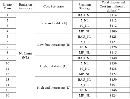
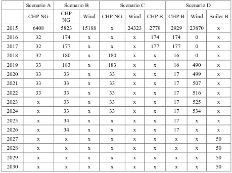
Table 5-1 Scenario description and the cost of optimal solutions under various strategies and scenarios . 51 Table 5-2 New capacities to be installed under MP_NL year planning strategy in various scenarios ... 52
Table 5-3 New capacities to be installed under 10_NL year planning strategy in various scenarios ... 54
Table 5-4 New capacities to be installed under annual investment limits ... 56
Table 5-5 Scenario description and the cost of optimal solutions under various strategies and scenarios . 59 Table 5-6 New capacities to be installed under MP_PR strategy ... 60
Table 5-7 Share of carbon offsets and RECs as a percentage of baseline carbon emissions ... 61
Table 5-8 Scenario description and the cost of optimal solutions under various levels of the percentage limits ... 62
Table 5-9 New capacities to be installed under MP_NL_100% and MP_PR_100% year planning strategy ... 63
Table 5-10 New capacities to be installed under MP_NL_50% and MP_PR_50% year planning strategy64 Table 5-11 New capacities to be installed under MP_NL_0% and MP_PR_0% year planning strategy ... 65
Table 5-12 Results of MCS ... 67
Table 9-1 Representation of Uncertainties in Electricity and Natural gas Prices ... 79
Table 9-2 Range of Carbon Prices ... 80
1
Chapter 1. Introduction
1.1 Motivation:
Increasing global environmental problems require a rapid response from universities (Sharp,
2002). Universities should not only be sustainable in their campus operations, but also provide
leadership for the broader society (Sharp, 2002). Electricity consumption of universities is
increasing due to, for example, expansion in use of electronics and new building constructions
(Levine, 2009; Sharp, 2002).
There are increasing numbers of initiatives on university campuses to address climate change.
The American College and University President’s Climate Commitment (ACUPCC) is an effort
by a group of colleges and universities that have pledged to eliminate greenhouse gas (GHG)
emissions from their campus operations and become carbon neutral by a target date set by each
university itself (ACUPCC, 2006). ACUPCC recommended that universities minimize GHG
emissions and use carbon offsets to neutralize the remaining emissions (ACUPCC, 2006).
Emissions reported in a GHG inventory are usually divided in three categories: Scope 1, Scope
2, and Scope 3 emissions (Klein-Banai & Theis, 2011). Emissions associated with on-site fuel
consumption are categorized as Scope1 emissions. Emissions associated with purchased heat,
cooling, steam, and electricity are considered as Scope 2 emissions. All emissions associated
with air travel, transmission and distribution losses associated with purchased electricity,
commuting, refrigerant, and waste are categorized as Scope 3 emissions (Klein-Banai & Theis,
2011). According to the analysis conducted by (Klein-Banai & Theis, 2011), Scope 1 and Scope
2 emissions constitute the majority of emissions in colleges.
The ACUPCC’ commitment requires each participating university to prepare a Climate Action
2
certain date set by the universities themselves (ACUPCC, 2006). According to (ACUPCC,
2006), the GHG inventory can provide a basis to develop a CAP because the inventory reveals
what and how much emissions are created through every campus operation. (Levine, 2009;
Simpson, 2009) propose a number of actions such as energy efficiency projects, renewable
energy projects, carbon credits, and renewable energy credits (REC) that universities can
consider to reduce their carbon footprint. A CAP should usually describe: i) which energy
alternatives should be installed; ii) what is the size of the alternatives that need to be installed;
iii) when should the alternative be installed during a given planning horizon. However, there is
no standard approach for developing a CAP, and many universities find it difficult to complete
such plans and they often lack the necessary resources for effective planning (Abbott, 2010;
Rizzoa & Savinob, 2012).
There are many energy saving opportunities on college campuses such as using ENERGY STAR
equipment, efficient lighting, and energy conservation that many universities have failed to
capture (Levine, 2009; Simpson, 2009). A campus can be made more energy efficient by
implementing such “low hanging fruit” projects that need modest capital investment and offer
significant energy savings. Therefore, universities may prioritize such actions for short-term
emission reductions. Simpson (2009) argued that universities usually prefer projects that have
short payback period and may ignore projects with longer payback period. Moreover, Levine,
(2009) suggested that there might be fewer such opportunities remaining in universities that have
been part of campus sustainability initiatives for a long period and may already have exploited
projects with quick payback period such as energy efficient lighting. According to Simpson
(2009), once all opportunities of short payback period are exhausted, it becomes difficult for
3
be financially unattractive. However, projects with longer payback are essential for substantial
reductions in GHG emissions (Simpson, 2009).
Another example of short-term thinking could be reliance on Renewable Energy Credits (RECs).
ACUPCC commitment allows universities to purchase RECs and carbon offsets to neutralize
their emissions (ACUPCC, 2006). Purchasing RECs may be an inexpensive way to reduce
carbon footprint associated with the purchased electricity and support the development of clean
energy sources. However, buying RECs may be cheaper in short-term, but may become
expensive in the long run (Simpson, 2009). Despite many benefits of RECs, some skeptics
argued that RECs purchasers receive nothing of value other than “bragging rights” (Simpson,
2009). Therefore, universities focusing on short-term benefits may be tempted to buy RECs and
refrain from investing in long-term renewable energy projects.
Among the sustainability problems that university decision makers face are limited financial
resources, emission constraints, and availability of a large number of energy supply options, and
large number of energy efficiency measures. Selecting the optimal combination of supply
options and efficiency measures is not an easy task. Uncertainties in future values of various cost
parameters further complicate the decision making process to find an optimal plan. (Awerbuch,
2000) argued that economic models that ignore uncertainties may favor cheap fossil fuel
technologies with cost streams that are very sensitive to fluctuations in the fuel prices over
capital intensive technologies such as photovoltaic with expensive but a uniform cost stream.
Usually, planning is done by assuming a single future cost scenario. Such analysis produces a
single optimal plan. However, there are a large number of possible cost scenarios due to the
4
value of various cost parameters also make it more complicated to find a lowest cost action plan
in long-term investment strategies because each scenario may produce a different optimal plan
(Awerbuch, 2000). According to Hobbs, (1995) it is possible to identify a robust plan that,
although not optimal, performs satisfactorily well under all or most of the possible scenarios if
uncertainties are also considered. There appears to be a need for methodologies that can help
universities design a CAP that meets requirements of their decision makers such as annual
budget constraints and environmental constraints. According to (Levine, 2009), decision makers
of a university should consider available resources, uncertainties, and their risk attitudes while
preparing their CAP. Financially risk-averse colleges may set interim as well as final goals they
are certain to meet (Levine, 2009).
Application of optimization models in determining multi-period optimal energy mix in an energy
system is not new. Several studies (Cormio, Dicorato, Minoia, & Trovato, 2003; Mirzaesmaeeli,
Elkamel, Douglas, Croiset, & Gupta, 2010) propose energy optimization models to determine
multi-period investment strategies for a typical energy system. The main purpose of such models
consists of determining what energy alternatives should be installed, what size of an alternative
should be installed, and how installed alternatives should be operated in order to satisfy energy
demand and environmental constraints in each period. These studies failed to account for
uncertainties in input parameters. Other studies use models based on Monte-Carlo Simulation to
account for risks in electricity and gas prices (Dicorato, Forte, & Trovato, 2008; Feretic &
Tomsic, 2005; Hawkes, 2010; Vithayasrichareon, MacGill, & Fushuan, 2009). However, these
studies focus on single period rather than multi-period investment planning. This thesis will
5
However, the model developed in this study will be capable of incorporating other types of
uncertainties as well.
1.2 Problem Statement
Suppose a university aims to determine what energy mix will satisfy partially or fully its
annual energy demand (heat and electricity) in an environmentally responsible way. The costs to
achieve carbon neutrality depend on the energy action plan of the institution. Each plan can be
composed of a selection of different options that may differ from each other in economic and
environmental factors. Some technologies such as fossil based generations have lower capital
costs, fuel costs, and higher emissions. Some technologies such as renewable energy have higher
capital cost, no fuel cost, and lower or zero emissions. In addition to generating energy,
universities can also purchase electricity from the grid. Renewable energy credits and carbon
offsets can also help to reduce carbon footprint of a university without investing in renewable
energy technologies.
Based on available options and their characteristics, decision makers are required to find optimal
contribution/share of each option in an energy plan. While developing an energy plan, decision
makers may prefer to divide the planning horizon into multiple short-term planning periods and
develop an optimal plan for each portion of that planning period. Such a strategy will produce
multiple short-term optimal plans, which may be sub-optimal through a perspective of long-term
planning period. On the other hand, decision makers may choose to develop an optimal plan by
considering the entire planning horizon as a single planning period. However, such long-term
plans may have high initial capital investments. There are financial constraints that must be met.
Some universities may not have adequate financial resources to make large capital investments,
6
In addition, some plans may be required to just focus on the ultimate goal of carbon neutrality
that will ensure zero emissions after a certain date without any regards to the annual emission
trajectory. Some plans may have additional constraints such as annual emission limits, which
will lead to a gradual emission reduction trajectory to carbon neutrality. Different emission
trajectories can have different impacts on the cost to achieve carbon neutrality (Mirzaesmaeeli et
al., 2010). There are various energy alternatives available to choose from that might fulfill these
constraints. However, developing an energy plan by selecting appropriate size and combination
of alternatives, while simultaneously satisfying various constraints under uncertainties, is a very
challenging task. Also, conventional practice of analyzing each single alternative independently
for its net present value or cost-benefit ratio may not be effective in developing an optimal
energy plan because there are many alternatives, and some of them are interdependent (George
Mavrotas, Florios, & Vlachou, 2010). Therefore, the universities can use optimization models to
develop an energy action plan that takes into consideration their objectives, budget constraints,
and environmental constraints. The modeling approach can also help university decision-makers
deal with the uncertainties.
Rizzoa & Savinob, (2012) asserted the importance of using linear programming models in
developing optimal energy plans. The authors showed that short-term and long-term planning
produce different optimal energy plans. The long-term planning required large capital investment
and had more long-term benefits than short term planning, which required small capital
investment. Several models have been proposed to study energy planning for an energy system
(Cormio et al., 2003; Mirzaesmaeeli et al., 2010; Rizzoa & Savinob, 2012). These proposed
deterministic models determine an optimal combination of energy options in an energy system
7
various uncertain factors such as long term utility prices and carbon prices make quantifying
actual cash flow for each plan uncertain. Therefore, under the budget and environmental
constraints, choosing the right investment plan using deterministic models alone is not only
difficult, but inadequate. This thesis proposes integrating the use of deterministic optimization
models (e.g. Linear Programs) into a Monte-Carlo Simulation experiment to properly deal with
planning uncertainties.
This thesis proposes and applies an optimization model to develop energy plan for Rochester
Institute of Technology (RIT) and produce experimental results to address the following research
questions:-
1) How and to what extent will the length of the planning period (no planning, every five
years, every ten years, or once in every 20 years) affect an energy plan?
2) How and to what extent will the annual emission and/or carbon offset targets affect an
energy plan?
3) How will an energy plan adopted for one particular scenario behave under different
future cost scenarios?
This study does not generalize the experimental results to the planning of energy investments
made by all universities, but it rather suggests an optimization based methodology that could be
used to enrich and improve energy supply planning.
The remainder of the thesis is organized as follows: - Chapter 2 provides a literature review.
Chapter 3 presents the section on methodology used to answer research questions mentioned
above. Chapter 4 provides an experimentation of the model. Chapter 5 provides an analysis and
8
Chapter 2. Literature Review
2.1 Mathematical Models in Energy Planning
Linear programming models are widely used tools in energy planning (Cormio et al., 2003;
Hobbs, 1995; G. Mavrotas, Demertzis, Meintani, & Diakoulaki, 2003; Mirzaesmaeeli et al.,
2010). A number of energy planning tools have been developed for national and regional level
energy systems (S. Awerbuch & Berger, 2003; Cormio et al., 2003; Mirzaesmaeeli et al., 2010).
There appears to be growing interest in applying similar models in the planning of small-scale
and building level energy systems (Jackson, 2008; George Mavrotas et al., 2010; Rizzoa &
Savinob, 2012). Some of these models consider uncertainties in input parameters (S. Awerbuch
& Berger, 2003; Feretic & Tomsic, 2005; Vithayasrichareon et al., 2009), but focus on one-time
investments. Some of these models do not consider uncertainties, but provide multi-year
investment plans (Cormio et al., 2003; Mirzaesmaeeli et al., 2010). However, there appears to be
a lack of studies that used energy models to analyze effects of uncertainties on multi-year
investments plans.
Mirzaesmaeeli et al. (2010) proposed a deterministic non-linear multi period model, which was
reduced to a linear model using an exact linearized method. George Mavrotas et al. (2010)
developed a MILP model for energy planning in a hotel and applied Monte-Carlo simulation
(MCS) technique to capture economic uncertainties. The model determines which and what size
of energy alternatives should be installed to minimize annualized costs while meeting heating,
cooling, and electricity load. George Mavrotas et al. (2010) conducted a case study in which
electricity price, natural gas price, and discount rate were considered to be uncertain. According
to the results, for a majority of the scenarios, a new Combined Heat and Power (CHP) unit was
9
numbers of scenarios when prices of natural gas were high and prices of electricity were low,
installation of CHP unit was not part of optimal solution. These results provide an interesting
insight. If a decision maker solves the model for single instance of input parameters by assuming
high gas prices and low electricity prices, then optimal solution would become sub-optimal in
many future scenarios. However, application of MCS can help the decision maker realize how
objective function and decision variables vary with the given uncertainties in the input
parameters (George Mavrotas et al., 2010).
S. Awerbuch & Berger (2003) and Roques, Newbery, & Nuttall (2008) applied the portfolio
approach to derive efficient energy portfolios for large energy systems. At any given time in an
energy portfolio, generation costs of some technologies are higher than the generation costs of
the other technologies in the portfolio. Over time, an optimal combination and share of
technologies in the portfolio minimizes overall generation cost of the portfolio relative to the
risk. Risk can be defined as yearly fluctuation in the generation costs of the technologies
(Awerbuch, 2000). Each efficient portfolio has some cost and risk associated with it. A decision
maker may choose any portfolio based on the risk attitude of the decision maker. However, the
portfolio approach assumes that the generation costs of various technologies are normally
distributed, which may not necessarily be true (S. Awerbuch & Berger, 2003).
Feretic & Tomsic (2005) used Monte-Carlo simulation to generate probability distribution of
levelized cost of energy from three different power plants: coal, nuclear, and natural gas.
Levelized cost of energy is defined as average cost of a unit of energy from a power plant over
its lifetime. Its unit is $/kWh. The authors used probability distributions to describe uncertain
input parameters such as investment cost, fuel cost, and operation life time of power plant. The
10
doubled after introducing external costs such as environmental costs. Cost of energy from natural
gas increased 30 percent due to external costs. One of the conclusions the authors drew was the
importance of environmental and social costs of power plants. Therefore, any energy planning
process should also consider environmental costs that may occur in future while evaluating
economics of an energy plan. However, the method proposed in (Feretic & Tomsic, 2005) uses
just Monte-Carlo Simulation, therefore, can only be useful in simulating generating cost of a
given energy technology under uncertainty rather than finding an optimal combination of
various technologies. Vithayasrichareon et al. (2009) proposed a linear programming model to
determine optimal operation of a portfolio by minimizing operational costs. The authors also
used Monte-Carlo Simulation to study the impact of various uncertainties on overall generation
cost of various portfolios composed of one or more of following technologies: coal, combine
cycle gas turbine, and open cycle gas turbine. The authors considered uncertainties in carbon
price, coal price, and gas price by representing those uncertainties by normal distributions.
Hawkes (2010) proposed a deterministic linear programming model to determine the optimal
installation capacity of various energy technologies in an energy system. The objective function
minimized equivalent annual cost (EAC) of energy system. The author conducted the experiment
in two steps. The first step performed deterministic optimization based on single estimates of
energy prices. The second step used Monte-Carlo Simulation (MCS) for the combination of
energy technologies obtained in the first step to account for uncertainties in electricity, natural
gas, and wind speed. The results obtained through MCS showed that the deterministic
optimization ignored economic risks. Therefore, it can be concluded that optimal solution based
on a single estimate of fuel prices may become suboptimal under different prices scenarios. A
11
Rizzoa & Savinob, (2012) presented a deterministic linear programming model suitable for
solving energy and environmental planning problems at small scale and municipal level. The
authors illustrated the application of model by describing an optimal resource allocation problem
to reduce emissions at school level. (Rizzoa & Savinob, 2012) also asserted that an optimal
solution for a particular objective could not simply be obtained by finding optimal solution that
meets half the objective, and then doubling the values of each decision variable to find the
solution to meet the complete objective. For example, a best strategy to reduce emissions by 100
percent was different from a strategy to reduce emission from 0 to 50 percent, and then doubling
the value of each decision variable. Therefore, according to the authors, the results implied that
the decision makers should have a clear picture of objectives and available resources at the
beginning of a planning horizon.
Cormio et al. (2003) proposed a dynamic linear programming model that finds the optimal mix of
energy technologies for an energy system. The objective was to minimize present cost of the
system over the entire planning period of 10-20 years. The system was subject to energy demand
and environmental constraints. This model was then applied to a regional energy system in Italy.
Mirzaesmaeeli et al. (2010) proposed a deterministic multi-period MILP model to determine
optimal-mix of generation technology that will meet energy demand and CO2 emission targets at
minimum cost. The objective function proposed seeks to minimize overall discounted cost over
the planning horizon. The model though comprehensive did not account for uncertainties in
future prices that would have affected investment decisions. As a college campus has a smaller,
but similar energy system as a regional energy system, a model similar to the models proposed in
(Cormio et al., 2003; Mirzaesmaeeli et al., 2010) can be formulated to study energy systems of
12
In summary, Feretic & Tomsic (2005), Hawkes (2010), George Mavrotas et al (2010), and
Vithayasrichareon et al. (2009) proposed energy models that consider uncertainties in various
input cost parameters. However, these models focus on one time investment strategies. Cormio
et al (2003), Mirzaesmaeeli et al (2010), and Zakerinia & Torabi (2010) proposed energy models
that provided multi-period investment strategies, but failed to consider uncertainties. This thesis
is proposing a deterministic multi-period optimization model to determine optimal mix of energy
technologies in a small-scale energy system for a given demand. Moreover, the model will
integrate Monte-Carlo Simulation (MCS) to account for uncertainties in electricity, natural gas,
and carbon prices.
This work will not optimize operational schedule of various alternatives as done in previous
studies (Cormio et al., 2003; Mirzaesmaeeli et al., 2010). The main reason for this limitation is
inclusion of non-dispatchable technologies such as wind and solar. Power production from these
13
Chapter 3. Methodology
3.1 Mathematical Programming
Mathematical programming is a tool for solving optimization problems. A typical
optimization problem has the following components (Winston & Goldberg, 1994):
i. Objective function: The objective function is the goal of the problem. It can be
minimize or maximize a criterion (costs or benefits) or multiple criteria
simultaneously (costs and risks).
ii. Decision variables: The decision variables describe decisions that have to be made in
order to solve the problem
iii. Constraints: Constraints are conditions that must be met by any solution. In other
words, constraints restrict the values decision variables can take.
Optimization problems can be represented by mathematical models, which try to determine
values of decision variables that minimize or maximize the objective function among the set of
all decision variables that satisfy given constraints. The constraints in most of the optimization
models used in the energy sector usually ensure the power and energy demand of an energy
system. Additional constraints such as technological limitations, environmental constraints, fuel
consumption limits, and size limits are also considered. Usually, addition of each new constraint
increases the cost of optimal solution. The decision variables in a typical optimization problem
related to energy investments are finding the optimal size of various energy technologies in a
given energy system, optimal operation of each technology, and/or sequence of additional
installations of each technology required in order to satisfy the constraints such as energy
demand (Hobbs, 1995). The typical objective in most of energy planning models is to minimize
14
system over the entire planning horizon (Hobbs, 1995). This chapter develops an energy
planning model that combines Mathematical Programming and Monte Carlo simulation in order
to address research questions described in the first chapter. Combining deterministic
mathematical models and Monte Carlo simulation is a challenging task. This work will use an
approach similar to the one described in (Feretic & Tomsic, 2005; Hawk, 2010). The
methodology is proposed in two parts. The first part develops a deterministic optimization model
to represent an energy system. The second part experiments with Monte Carlo simulation based
on the findings of the first part to account for uncertainties.
3.2 Model Formulation
This section describes a model, which is a multi-period deterministic Linear Programming
(LP) model. The section (3.2.1) details the various sets and notations used in the model. The
model finds the values of decision variables (see section 3.2.3) such as capacities of energy
alternatives that need to be installed and energy to be bought over a given planning period. The
various constraints are described in section (3.2.5). The main constraints incorporated in the
model include need to meet annual energy demand (3.2.5.1) and emission restrictions (3.2.5.4).
In order to keep the model simple and tractable without reducing its ability to address the
research questions, it assumes that there is no year-to-year variability in energy generated from
wind and solar. A typical power production1 modeling of an energy system requires time
resolution of one hour. However, hourly analyses of intermittent and unpredictable energy
technologies such as solar and wind can make a model intractable. Therefore, this model
analyzes annual energy generation and demand only. Also, the main aim of an energy plan for a
1
15
college campus is to meet the energy demand at minimal most; therefore, option to export excess
electricity back into the grid is not included.
3.2.1 Sets and Indices:
Notation ‘I’ is used to represent the set of different types of primary fuel available to meet
energy demand. The set of various alternatives that are available is represented by notation ‘B’.
Each fuel-based alternative transforms primary energy into a secondary form of energy, which is
either heat, electricity, or both. The secondary form of energy is used to meet the energy demand.
Non-fuel based alternative such as wind and solar directly produces secondary form of energy,
which can be used to meet the energy demand. Set ‘W’ represents different types of energy
demand.
Set represents set of primary fuel
- Natural gas
- Biomass
Set represents set of different energy alternatives
fuel based generation
- CHP_NG (natural gas fired)
- CHP_B (biomass fired)
- Boiler_NG (natural gas fired)
- Boiler_B (biomass fired)
Non-fuel based energy alternatives
- Wind
16
Set represents set of different types of energy demand
- Electricity
- Heat energy
Set represents time period in years (t= 0, 1, 2, 3….19 representing time period 2015 to 2034)
3.2.2 Parameters:
This section describes the parameters that were used in the model. Different types of input
data were represented by different types of parameters. The parameters used in our work can be
classified into three main categories: cost parameters, technical parameters, and constraint
parameters.
The following is the list of notations used to represent the cost parameters followed by a small
description about each parameter.
- Investment cost of alternative in period ($/unit)
- Fixed operation and maintenance cost of alternative in year ($/unit)
- Variable O&M cost of alternative in year ($/unit)
- Price of fuel in year ($/MMBtu)
- Price of purchased energy type in year ($/MMBtu)
- Price of renewable energy credits energy type in year ($/kWh)
- Financial incentive for alternative in year ($ or $/kW or $/kWh)
- Carbon credit price in year ($/ton of CO2 equivalent)
- Real discount rate
The following is the list of notations used to represent technical parameters followed by a small
description about each parameter. The technical parameters were used to represent technical
17
- Capacity factor of alternative
- Conversion efficiency of alternative w.r.t. energy
- Output energy coefficient of alternative
if alternative b produces w type of energy, 0 otherwise
- Operational life time of alternative (years)
- Lead time of alternative (years)
- Large Number
The following is the list of notations used to represent constraint parameters followed by a small
description about each parameter. The constraint parameters were used directly or indirectly to
represent information related to resource constraint, size constraint, or environmental constraints.
- Capacity of alternative existing at the beginning of planning horizon and still
operational in year (units)
- Lower limit on total capacity of alternative
- Upper limit on total capacity of alternative
- Lower bound on minimum size of alternative
- Upper bound on maximum size of alternative
- Demand of energy type in year (kWh)
- GHG emission from unit consumption of fuel (kg of CO2/unit)
- Carbon footprint of purchased energy type in year (kg of
CO2/MMBtu)
- Limit on GHG emissions in year (kg of CO2 equivalent)
18
3.2.3 Decision Variables:
- If an alternative should be installed in year (0 if no, 1 if yes)
- New installation capacity or size of alternative in year (kW or kWth)
- Annual energy type produced from alternative in year
(kWh)
- Amount of energy type purchased in year (kWh)
- Amount of fuel used by alternative in year (kWh)
- Renewable energy credits for energy type purchased in year
(kWh)
- Carbon credits purchased in year (tons of CO2 equivalents)
3.2.4 Objective Function
The goal of this model is to determine how much and when to invest in each alternative of an
energy system, subject to energy demand and emission constraints. Our objective minimizes the
sum of the present value of annual energy expenditures occurred during the each year of the
specified planning horizon. The following expression provides a mathematical formulation of the
objective function.
∑
The term represents total annual cost associated with energy in year t. The annual cost can
be broken down into the following cost components.
+ + + + + + -
Where, is total investment cost occurred in any year and is calculated by equation (3.2).
19
depends on type and size of alternatives installed and their capital cost. In the following
equation, represents the type and size of alternative installed in year ‘t’ and represents
respective capital cost.
∑
It is assumed that there is no difference between O&M costs of older equipment and newer
equipment. Though it may not necessarily reflect reality as older equipment has higher
maintenance cost that an equivalent newer one, this assumption is necessary to keep the
tractability of the model. Equipment that retires during the planning horizon will not incur any
operation and maintenance costs beyond their useful life. Also, it is assumed that the equipment
that is still under construction will not have any operation and maintenance costs until it starts
producing energy. Therefore, in any year , set limits the installed capacity that has been
commissioned by the beginning of the year and still in operation in the year. is operational
life of an alternative b. is the lead time of installation for alternative b.
[
and represent fixed operation and maintenance and variable operation and
maintenance cost occurred any year t. These costs can be obtained by expressions (3.3) and (3.6)
respectively. is the total capacity of an alternative that was installed before planning period
begun and still operational in year t. is the total installed capacity of an alternative that is
operational in year t.
20
The variable operation and maintenance (VOM) cost depends on the energy produced by an
alternative ( in any energy t. The VOM is represented by two components. The first
component (3.4) calculates VOM costs of non-CHP alternatives. The second component (3.5)
calculates VOM cost of CHP alternatives. The VOM of CHP technologies is expressed in terms
of electricity production only. Therefore, constraint (3.6) accounts for total cost, which is
sum of these two components.
∑ ∑
∑ ∑
represents cost of energy purchased from utilities in year t. It depends on amount of
each type of energy purchased ( and its price ( in that year. It can be calculated by
expression (3.7).
∑
The cost component associated with fuel costs incurred in year t is obtained by expression (3.8).
The fuel costs are dependent on fuel prices ( and amount of fuel used ( in that year.
∑ ∑
cost component represents the cost of purchasing renewable energy credits, and can
be obtained by expression (3.9). It can be calculated by multiplying amount of energy credits
purchased ( and the price of each credit ( .
21
The expression (3.10) calculates cost of purchasing carbon credits in year t. It depends on
amount of carbon credits purchased ( and its price ( in that year.
represents the total financial incentive/grants/tax benefits received from any entity
for each alternative.
∑
3.2.5 Model Constraints
3.2.5.1Energy Production and Demand
The following constraint (3.12) ensures that the total annual energy production (AEB) of
each type of energy is more than the demand of that type of energy in any given year in the
planning period. The energy supply includes on-campus energy generation by alternatives
( and energy purchase ( . The overall energy demand ( is assumed to be
known for each year.
∑
It is also assumed that the performance of any alternative does not degrade over time. It means
that older equipment will perform just as well as an equivalent newer one.
3.2.5.2 Maximum Energy Production
In any given year, the energy produced by an alternative ( cannot exceed its
maximum energy generation capacity. The output energy coefficient ( in constraint (3.13) is
multiplied to impose an upper limit on the kind of energy the alternatives (5 and 6) can supply.
22
Additional constraints (3.14) and (3.15) ensure that the energy generated from fuel-based
alternatives does not exceed maximum possible generation from total installed capacity2. A
Combined Heat and Power (CHP) technology is rated in terms of electricity production capacity.
Therefore, heat recovery from a CHP technology is dependent on amount of electricity produced
by that technology. Therefore, constraint (3.12) is defined over single index (w=1) only. 8760
represents number of hours in a year.
( ∑ )
( ∑ )
The constraint (3.16) ensures that the energy generated from alternatives (1, 2, 3, and 4) is in
balance with the annual fuel consumption by the alternatives. It should be noted that the
constraint (3.16) also makes sure that ratio3 of heat and electrical power by CHP alternative is in
accordance with the characteristics of the CHP technology. It is assumed that this ratio remains
unchanged throughout the operational phase of CHP alternative. In constraint (3.16) the number
293 represents unit conversion factor: 1MMBtu=293kWh
∑
3.2.5.3 Maximum Capacity Constraint
The total installed capacity of any alternative should be within its allowable limit. The
constraint (3.17) will keep the total installed capacity of an alternative above its minimum limit
and below its upper limit. The minimum limit can be defined by decision makers. For example,
2 Inequality in constraint (3.12, 3.13, and 3.14) is modeled to include all feasible solutions. However, it is always
sub-optimal to utilize less energy than what is available if money has already been invested to install new capacity.
3
23
there can a requirement to have at least some photovoltaic or wind turbines in energy systems
even if they are not cost effective.
∑
[
Rizzoa & Savinob (2012) recognized that there are certain economy-of-scale issues in small scale
energy systems related to size of energy alternatives that affect unit cost. The relationship
between size and unit cost is often non-linear, which can be approximated by linear relationships.
The authors suggested that each size-scale (for example small, medium or large) of every
generation technology can be considered as a separate decision variable. Each size-scale can be
represented by a range where size and unit cost exhibit linear relationship. Furthermore, George
Mavrotas et al., (2010) also used similar piecewise linear approximation as described in
constraints (3.18 and 3.19) to account for non-linear cost-size relationship. The decision variable
and in the constraints express whether or not an alternative should be installed in any
given year and what capacity should be installed respectively. The parameters and
capture the range of values the decision variables are allowed to take without violating
linearity assumption.
Constraint (3.20) limits the amount of renewable energy credits ( ) purchased, which
cannot exceed the amount of purchased energy ( . Factor ‘1000’ in (3.20) is conversion
24
3.2.5.4 Emission Constraint
Total carbon footprint of the system should not exceed annual carbon footprint limit
( on the system imposed by decision maker. The following constraint accounts for
emissions associated with burning of fuel. It depends on fuel use ( , amount of emissions
emitted by burning one unit of fuel ( in boilers, amount of energy purchased ( and
carbon footprint of purchased energy ( . Purchasing Renewable Energy Credits ( )
can reduce the carbon footprint associated with purchased energy. Additionally, overall carbon
footprint of the system can also be reduced through carbon credits ( . One carbon credit is
equivalent to 1000kgs of CO2. Constraint (3.22) limits share of carbon offsets and RECs towards
meeting the emission targets. This constraint can indirectly increase the share of renewable
energy in an energy system.
∑ ∑ ∑
∑
3.2.5.5 Fuel Use Constraint
Any boiler or CHP unit is assumed to use only one type of fuel throughout its operation. The
following constraint will ensure that no boiler uses multiple fuels in any year.
25
3.3 Monte Carlo Simulation (MCS)
There are multiple ways to analyze uncertainties in input parameters. Some of the ways to
analyze uncertainties are sensitivity analysis and scenario analysis. Sensitivity analysis measures
the change in output variable with respect to change in values of input parameters one at a time
(Spinney & Watkins, 1996). One of the strengths of sensitivity analysis is that it can be helpful in
screening the parameters that have biggest impact on the output. However, one of the limitations
of using sensitivity analysis is that it analyzes only one uncertain parameter at a time. Such
analysis may ignore the interaction among various input parameters.
Another way to analyze uncertainties is scenario analysis. Decision makers can analyze multiple
scenarios to account for uncertainty. One common ways to classify scenarios can be ‘best case’,
‘base case’, and ‘worst case’ scenario (Spinney & Watkins, 1996). Each scenario is associated
with a particular combination of input parameters. The advantage of using scenario analysis over
sensitivity analysis is that decision makers can analyze impacts on the output by changing
multiple uncertain parameters simultaneously. However, drawback of this approach is that if
uncertainties in input parameters are large, or there are too many uncertain parameters are large,
the number of possible scenarios can be very large.
Monte Carlo simulation (MCS) is a very helpful way to experiment with a large number of
possible combinations of input parameters (Spinney & Watkins, 1996). In MCS experiment, all
input parameters are expressed as probability distribution. Then, the experiment is run for a
certain number of trials. In each trial, the value of each uncertain parameter is randomly chosen
from its probability distribution to find corresponding value of the output. Repeating the process
26
advantage of using MCS is that it also gives information on the distribution of the output as
compared to scenario analysis, which only gives a range of values of the output.
In an energy planning, there can be many uncertain parameters such as, but not limited to capital
costs of wind and PV, electricity, gas, and carbon prices. As number of uncertain parameters or
range of uncertainties in the values of some parameter increases, choice of MCS over scenario
analysis can be very helpful in determining cost distribution of an energy plan.
In the existing literature on energy planning, MCS technique has been used in two different
ways. George Mavrotas et al (2010) used Monte Carlo simulation to solve the optimization
model by randomly choosing values of input parameters from their respective probability
distribution. The results of objective function and decision variables are recorded after each
repetition of the simulation. In this type of application, MCS produces a probability distribution
of the objective function and decision variable by repeated sampling of the input parameters.
Therefore, the decision maker can see how the objective function and the decision variables can
vary, given the specific uncertainty on the model’s parameters. With this type of application of
the simulation users can explore and understand which decision variables are important and
which have negligible effects on the system under uncertainty. However, choosing an
appropriate set of decision variables from the distribution is challenging. Also, further
experimentation must be done in order to describe how a particular energy plan will behave
under uncertainty once a particular set of decision variables (combination of energy alternatives)
has been chosen.
Hawks (2010) applied MCS technique to analyze economic performance of a single combination
of technologies. In this type of application, simulations were performed by repeated sampling of
27
with a single estimate of uncertain parameters through deterministic optimization. The output of
the simulation was the distribution of objective function, which was savings in energy cost.
In our work, the second type of application can be more useful in determining economic
behavior of one particular mix of technologies under uncertainty. The Monte Carlo simulation
experiment conducted in this thesis is similar to the application proposed in Hawks (2010). We
aim to use MCS to find how the total cost of a particular energy plan (combination of energy
alternatives or technology mix) may be affected by uncertainties in input parameter. In this
study, we limit our analysis to only three uncertain parameters, electricity, natural gas, and
carbon prices to test the effectiveness of MCS in energy planning. The next chapter applies the
methodology to develop energy plan for an energy system.
28
Chapter 4. Experiment
The methodology described in the previous chapter has two parts. The modeling part that
finds the values of decision variables (energy plan) such as capacities of energy alternatives that
need to be installed and energy to be bought over a given planning period for a particular cost
scenario. Monte-Carlo Simulation experiment, then, helps to assess the effects of uncertainties in
natural gas, electricity, and carbon prices on an energy plan. This methodology can be useful for
universities interested in assessing the effects of certain aspects of energy planning such as the
length of the planning period, uncertainties in costs, and certain constraints on investment
decisions. This methodology mainly requires snapshot of existing energy system, knowledge of
future annual energy demand of campus that must be satisfied, and types of fuel and energy
alternatives available to decision makers in order to meet the energy demand. Uncertainty
analysis requires knowledge of probability distribution of uncertain parameters. In order to
answer the research questions mentioned in the first chapter, the methodology was tested through
its application to develop an energy plan for Rochester Institute of Technology (RIT) campus.
The following section (4.1) provides details on RIT campus and its energy system. The next
section (4.2) discusses what the most likely decisions are that RIT may have to make in order to
develop its energy plan. It also describes how the experiment was set up and all the scenarios that
were considered. The last section (4.3) of this chapter provides the data on energy system of RIT,
29
4.1 Background Information on the Campus
RIT is a private university located in suburban Rochester. Its campus occupies 1300 acres of
land (RIT, 2012b). In the past few decades, student enrollment increased by more than 20-30
percent (RIT, 2012b). RIT offers many doctoral, masters, and bachelor level degree programs.
Moreover, many more additional new programs and courses are now being offered. Many new
construction projects such as Institute Hall, Institute for Sustainability, and Gene Polisseni Arena
have already been completed or about to be completed in near future (RIT, 2012a) . Therefore,
due to the increasing size of campus and increment in student enrollment, RIT faces
sustainability challenges such as increasing energy consumption, waste generation, and
environmental emissions. Rising costs of electricity and natural gas can also put additional
financial burden on the university’s budget. Currently, the university spends more than $10
million on utilities annually (RIT, 2012c).
Share of Greenhouse Gas (GHG) emissions resulting from various activities related to the
campus is shown in figure 4-1. The majority of RIT’s greenhouse gas emissions in 2010 resulted
from purchased electricity, associated transmission and distribution loss, and combustion of
natural gas on campus (RIT, 2011). Emissions resulting from commuting and travel also
constitute a large portion of overall emissions. However, these emissions, which are considered
Scope3 emissions, are beyond the scope of this work because policies or initiatives focusing on
reducing Scope1 and Scope2 emissions may have little impact on Scope3 emissions and
vice-versa. Emissions related to commuting can be reduced through a green transportation policy
30
RIT pledged to become carbon neutral by the end of year 2030 (RIT, 2011). One of the main
focuses of RIT is to develop a list of projects and implementation timeline for those projects that
will reduce carbon emissions. Some of the actions RIT may take in the future to reduce its
emissions include investments in renewable energy and natural gas based power plants in
addition to improving energy efficiency. The goal of becoming carbon neutral can be met
through different ways. These ways include producing all energy through renewable energy
sources, purchasing carbon offsets and RECs, or in combination of both. However, renewable
energy requires large capital investments, which might limit the implementation of some of the
projects. On the other hand, strategy of relying just on carbon offsets and RECs to meet the goal
may turn out be expensive in the long run if carbon and RECs prices rise in the future. Therefore, Source: (RIT, 2011)
31
decision makers may have to find a desirable combination of these two ways to meet long-term
targets. Therefore, it also becomes necessary to invest in term projects, which requires
long-term planning because some of those decisions must be made much sooner than the target-date.
Therefore, decision makers at RIT need to compare costs associated with long-term planning
strategies and short-term planning strategies and also analyze uncertainties in various parameters.
The following section explores importance of such decisions using methodology proposed in
previous chapter to help decision makers at RIT to find an optimal alternative mix (energy plan)
that can meet their emission objectives and financial constraints.
4.2 Analysis Method
Suppose decision makers at RIT want to reduce their emissions related to energy
consumption. They are looking for the cost effective ways to meet their emission targets and
energy demand. In other words, they need an energy plan. An energy plan basically describes
what projects should be implemented and when they should be implemented. However, before
making any planning decisions to develop an energy plan, they must consider exploring costs of
some of the planning strategies. These planning strategies include length of planning period,
annual investment limits, and rate of annual emission (basically share of carbon offsets and
RECs). It is possible that choosing different planning strategies individually or combining
multiple strategies together, will result in different energy plan and different planning decisions.
Also, decision makers must also consider uncertainties in various parameters such as electricity
prices, natural gas prices, and carbon prices before making any large capital investments.
Next section describes the experimental setup. It was assumed that the energy demand reflected
the improvements achieved through energy efficiency and conservation. However, if decision
32
alternatives to find optimal mix, it can be achieved by considering energy efficiency and
conservation projects as alternatives in the model. This will require much more data on each
individual energy efficiency or conservation project. The planning horizon was assumed to span
from the starting of year 2015 to the end of year 2034, a period of 20 years. The deadline to
achieve carbon neutrality was by the end of year 2030.
4.2.1 Deterministic Analysis
Main purpose for this analysis was to test the effects of length of planning period, annual
investment limits, and rate of annual emission reduction on planning decisions by comparing
total present costs associated with each type of planning strategy. The analysis approach taken in
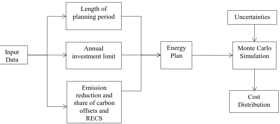
[image:43.612.60.523.364.569.2]this work is shown in figure 4-2
Figure 4-2 Analysis Method
4.2.1.1 Length of Planning Periods
Length of the planning period can be an important part of planning strategy. A planning
period is length of time period shorter or equal to the planning horizon. Decision makers may
choose to plan for different length of planning periods (every five years or ten years) to develop Length of
planning period
Annual investment limit
Emission reduction and share of carbon
offsets and RECS Input
Data
Energy Plan
Uncertainties
Monte Carlo Simulation
33
an energy plan. A solution which is optimal during a particular planning period may not be
optimal if analyzed over the entire planning horizon. Five or ten year planning approach will find
a solution that is optimal (the lowest cost solution) based only on five or ten year of data
respectively. Therefore, using either five year or ten year planning approach decision makers will
have to run the model sequentially four times (once in every five years) or two times (once in
every ten years) during the planning horizon of 20 years. Decisions in next five or ten years will
depend on decisions taken in previous five or ten years. On the other hand, 20 year planning
approach (MP) will find a solution based on analysis of 20 years, and decision makers will have
to run the model only once to find optimal solution. The deterministic optimization model was
used to find optimal energy plans for RIT through different planning period strategies for a
certain number of known cost scenarios (total four cost scenarios described in section 4.3.3). For
each of the cost scenarios and each of the planning period strategies, an optimal energy plan was
developed. Then total present costs associated with each of the optimal plan were compared to
draw conclusions.
4.2.1.2 Limit on Annual Investment
Long-term energy plans require may huge capital investments. In reality, due to resource
constraints it may not be possible to implement energy plans that require significant capital
investments. Suppose decision makers limit their maximum annual investments to certain
amount. The decision makers may not either have or be willing to invest large capitals. They
might be interested in making more gradual investments. This approach may give them more
flexibility because as more data become available on energy demand, cheaper energy
alternatives, or energy prices, it might be easier to adopt partially or fully better energy mix of