1
1
Special issue of Climatic Change 2
3
Natural hazards in Australia: storms, wind and hail
45
6
Kevin Walsh1, Christopher J. White2,3, Kathleen McInnes4, John Holmes5, Sandra Schuster6, Harald 7
Richter7, Jason P. Evans8, Alejandro Di Luca8, Robert A. Warren9 8
9
1* School of Earth Sciences, University of Melbourne, Australia 10
2 School of Engineering and ICT, University of Tasmania, Australia 11
3 Antarctic Climate and Ecosystems Cooperative Research Centre, University of Tasmania, 12
Australia 13
4 CSIRO Marine and Atmospheric Research, Australia 14
5 JDH Consulting, Mentone, Australia 15
6 Consultant, Sydney, Australia 16
7 Australian Bureau of Meteorology, Melbourne, Australia 17
8 Climate Change Research Centre & ARC Centre of Excellence for Climate System Science, 18
UNSW, Australia 19
9 Monash University, Australia 20
21
*Corresponding author’s address: Kevin Walsh, School of Earth Sciences, University of Melbourne 22
3010 Victoria, Australia. [email protected] 23
24
Manuscript Click here to download Manuscript 16_Walsh et
al_Wind-Hail-revised_final_textonly.docx Click here to view linked References
Abstract
25Current and potential future storm-related wind and hail hazard in Australia is reviewed. 26
Confidence in the current incidence of wind hazard depends upon the type of storm producing the 27
hazard. Current hail hazard is poorly quantified in most regions of Australia. Future projections of 28
wind hazard indicate decreases in wind hazard in northern Australia, increases along the east coast 29
and decreases in the south, although such projections are considerably uncertain and are more 30
uncertain for small-scale storms than for larger storms. A number of research gaps are identified 31
and recommendations made. 32
33
1. Introduction
34Natural hazards associated with storms, such as severe wind and large hail, cause significant 35
economic damage and social dislocation across Australia. For example, the high winds from 36
Cyclone Tracy (1974) caused an estimated A$2 billion dollars in damage (1999 dollars; BTE 2001). 37
Similarly, the insured cost of the 1999 Sydney hailstorm was estimated to be A$1.7 billion in 1999 38
dollars (RMS 2009). 39
Despite the severity of the impacts wrought by storms, there are limited reliable observed data for 40
some types of storms and associated hazards, particularly for the estimation of current wind hazard 41
from thunderstorms (section 2.2) and hail (section 2.3). Moreover, projections of future storm 42
characteristics have important uncertainties associated with them (section 4), while for hail, 43
projection studies have been few (section 4.2). Nevertheless, important progress has been made. To 44
summarise the latest knowledge and understanding of Australian storms, this paper reviews the 45
current scientific literature on the assessment, causes, observed trends and future projected changes 46
of storm hazard in Australia, with a specific focus on severe wind and hail hazard. The 47
meteorological causes of severe wind and hail are first outlined, including their geographical 48
distribution and methods of measurement, followed by observed trends. Future projections of these 49
hazards are then detailed, along with the uncertainties in these projections, concluding with 50
principal findings and some key open knowledge gaps and recommendations on future research 51
priorities. 52
53
2. Understanding wind and hail hazards
542.1 Storms that produce severe wind and hail
55
“Storms” are here defined as weather systems that produce severe wind and hail but their 56
occurrence varies from region to region in Australia. In the mid-latitude regions of Australia’s 57
south, extreme winds are produced by severe thunderstorms and intense extra-tropical cyclones 58
(ETCs), including their cold fronts. In the tropical regions of Australia, the largest contribution to 59
wind hazard is from tropical cyclones (TCs), with wind hazard from these systems occasionally 60
extending as far south as northern New South Wales (NSW) on the east coast and the Perth region 61
in the west. In addition to wind hazard, TCs can cause storm surge (which is discussed in the 62
companion coastal extremes paper, McInnes et al. (this issue)), flooding (which is similarly 63
discussed in Johnson et al. (this issue)), landslide damage and tornadoes. The east coast of Australia
64
from eastern Victoria (VIC) to southeastern Queensland (QLD) is subject to heavy rain, strong 65
winds and large waves resulting from coastal low pressure systems that develop from a variety of 66
weather systems (Speer et al. 2009). Generally referred to as East Coast Lows (ECLs), they cause a 67
significant amount of damage along the east coast each year. In the alpine areas, mountain wave 68
activity can lead to destructive winds on the downwind side of a ridge line under specific 69
meteorological conditions (Reinecke and Durran 2009), for example, at Thredbo valley in 2014 70
(pers. comm. including site inspection; http://www.abc.net.au/catalyst/stories/4117934.htm). 71
Severe thunderstorms are convective systems defined by the Australian Bureau of Meteorology to 72
be accompanied at least one of the following: 73
Hailstones with a diameter of 2 cm or more 74
Wind gusts of 90 km/h or greater 75
Flash flooding 76
Tornadoes 77
Storms that produce large hail and/or damaging winds (including tornadoes) typically form in 78
environments with significant thermodynamic instability and strong vertical wind shear (large 79
changes in wind speed and direction with height). In Australia, the highest incidence of these 80
systems is reported along the central and southern portions of the east coast (e.g. Allen et al. 2011, 81
their Fig. 1a). 82
2.2. Assessing current wind hazard
83
The strongest wind hazard is in the tropical regions of the country, where TCs occur. For the design 84
and assessment of buildings and structures, the region of influence of TCs is deemed to be coastal 85
strips as far south as 27oS on both the Western Australia (WA) coastline, and on the east QLD coast 86
(Standards Australia 2011). Based on the predicted effects of global warming (see section 4), these 87
boundaries may need to be extended further south (Holmes 2008, 2011; Kossin et al. 2014)
88
Since the 1960s, the ‘standard’ method of making estimates of return periods for high wind speeds 89
(i.e. for low annual probabilities of exceedence) has been based on recorded or ‘historical’ data, to 90
which the Type I Extreme, or Gumbel, probability distribution has been fitted (e.g. Coles et al. 91
2001). This distribution suffers from the disadvantage that it produces extreme values with no upper 92
limit: that is, continually increasing values of wind speed are generated as the return period 93
increases. From the 1990s onward, the less conservative Type III Extreme Value Distribution has 94
been used in Australia (Standards Australia 2011). This distribution produces predictions that 95
slowly asymptote to a (very) high upper limit, which is physically more realistic. 96
In Australia, the only recorded wind data that can realistically be used to assess extreme wind 97
speeds is the daily maximum gust that has been recorded by the Bureau of Meteorology since the 98
1940s, mostly at the standard height of 10 metres above flat, open country. These data are not 99
temporally homogeneous. In the 1990s, the conversion from the Dines anemometer (approximately 100
0.2 second gusts) to Automatic Weather Stations (AWS) with cup anemometers (digitally filtered to 101
3-second gusts) resulted in a discontinuity in the database, with the later AWS extreme gusts being 102
on average 10-20% lower than the earlier values, although conversion factors between the two have 103
been established (Holmes and Ginger 2012; Miller et al. 2013). These issues have affected efforts to
104
develop high quality surface wind data sets (Jakob 2010). 105
In many parts of Australia, high gusts are generated by more than one storm type – for example, in 106
the Sydney area both short duration thunderstorms and longer duration, synoptic-scale events, such 107
as ECLs, can produce high gusts. It is advisable, and good practice, for gusts produced by different 108
storm types to be separately analysed when carrying out extreme value analysis for a site. 109
Clearly, making estimates of extreme wind speeds at return periods of the order of hundreds of 110
years (which is usual for the design of structures against collapse or overturning – the so-called 111
‘ultimate limit states’) will result in significant sampling errors, when data for an individual 112
recording station is only available for 30-40 years. This can be partially alleviated in practice by 113
combining data from several stations in the same general location into a single ‘super-station’ (but 114
see Palutikof et al. 1999 for a discussion of the limitations of this methd). 115
Nevertheless, at locations where the occurrence of storms of a certain type are infrequent – for 116
example TCs at Cairns, QLD – the use of recorded gust data to make long-term return period 117
estimates will give very unreliable results. An alternative approach has been developed since the 118
1970s, based on simulating thousands of storms with the characteristics of those in the general area, 119
for example the Coral Sea in the case of Cairns. These methods generally consist of a combination 120
of probabilistic components (e.g. for the central pressure of TCs) and deterministic components 121
(e,g. for the wind field model associated with a tropical storm) (e.g. Harper 1999). A similar 122
approach is adopted for the impact of smaller storms such as thunderstorm downbursts or tornadoes 123
on physically large systems such as a transmission line several hundred kilometres in length (e.g. 124
Oliver et al. 2000). 125
The ability to estimate the current hazard accurately varies between storm types. Wind and hail 126
hazard from severe thunderstorms can be difficult to estimate over a large region. The main source 127
of data for severe thunderstorm incidence is reports provided by a network of observers, many of 128
whom are members of the general public. This record is spatially and temporally inhomogeneous 129
(Allen et al. 2011). The size of severe thunderstorms, typically less than 50 km in diameter, means 130
that they are not well observed in the sparsely populated regions of Australia. Meaningful 131
climatologies based on severe thunderstorm reports have been constructed in other parts of the 132
globe but these are typically in regions of higher population and data density (e.g. Doswell et al.
133
2005). Allen and Karoly (2014) circumvented this underreporting problem by instead examining the 134
incidence of larger-scale meteorological conditions conducive to the generation of severe 135
thunderstorms (that is, favourable “storm environments”), based on previous similar approaches 136
such as that of Brooks et al. (2003). They calibrated their severe thunderstorm thresholds with 137
available reports of severe thunderstorms in densely populated regions. A limitation of this 138
technique is that it estimates only the potential for formation of severe thunderstorms and is not an 139
accurate estimate, since their technique relies on probability assessment based on sparse data. 140
Observations of lightning can also provide insight into the occurrence of hazardous convective 141
weather, including damaging winds. Studies from the USA have demonstrated a clear link between 142
an increase in lightning flash count (so-called lightning “jumps”) and the onset of severe weather 143
(e.g. Schultz et al. 2011). However, to date, lightning data in Australia have only been used to 144
examine the distribution of all thunderstorms (Dowdy and Kuleshov 2014) and not specifically 145
severe storms. 146
Tornadoes are a particularly violent form of severe winds that are produced mostly by supercell 147
thunderstorms, long-lived thunderstorms that have their own small cyclonic circulation 148
(“mesocyclone”). Supercell tornadoes have been studied extensively in U.S. through two dedicated 149
field campaigns (VORTEX1; Rasmussen et al. 1994; VORTEX2; Wurman et al. 2012) and many
150
observational and numerical studies. In Australia, some tornado case studies have been published 151
(e.g., Hanstrum et al. 2002; Richter 2007), but the composition of a meaningful tornado climatology 152
is still a work in progress, as it involves the painstaking collection and evaluation of disparate 153
information sources such as newspaper articles (Allen and Allen 2016). 154
ECLs are phenomena with relatively small spatial scales (often smaller than TCs) and short 155
lifetimes (Holland et al. 1987), and their pressure centres may develop or intensify offshore making
156
them difficult to study using standard in situ observations. It has been known for some time that 157
ECLs produce large precipitation and wind events on the east coast of Australia (e.g. Holland et al.
158
1987; McInnes et al. 1992; Hopkins and Holland 1997; Mills et al. 2010). Moreover, ECLs have 159
the capacity for rapid intensification (Holland et al. 1987), and thus have been found to satisfy the 160
“Bomb” or rapid intensification criterion (a central pressure fall of 24 hPa in 24 hours) of Sanders 161
and Gyakum (1980). 162
The specific way in which ECLs are defined and the methodology used to identify and track these 163
cyclones varies considerably. The earlier work of Hopkins and Holland (1997) employed an 164
objective technique that combined wind and rain signatures typical of ECLs, as verified by 165
comparison with surface charts. Recent studies have used approaches based on expert judgment 166
(Speer et al. 2009), and various automated techniques that either track low pressure systems (Pepler 167
and Coutts-Smith 2013; Browning and Goodwin 2013; Di Luca et al. 2015) or identify favourable
168
conditions for their formation (Dowdy et al. 2013b). Pepler et al. (2014) investigated the 169
differences in ECL characteristics obtained using three different identification methods, finding that 170
the methods concur for relatively large and strong ECL events (including those producing high 171
winds) but diverge for smaller ECLs. While few studies have focused specifically on the wind 172
hazard associated with ECLs, the various measures used to characterize the intensity of ECLs, such 173
as the pressure gradient around the centre or the maximum cyclonic vorticity, are related to the 174
wind and hence changes in these intensity measures are expected to reflect changes in the wind. 175
At higher latitudes, for ETCs and their associated cold fronts, wind hazard can be estimated 176
reasonably well from Bureau of Meteorology wind data, as ETCs are more common than TCs. 177
Higher return period winds from ETCs have considerably lower accuracy, however. 178
2.3 Assessing current hail hazard
179
Current estimates of the hail hazard in Australia are available only from the Bureau of 180
Meteorology’s severe-storm archive (SSA; http://www.bom.gov.au/australia/stormarchive/). As 181
previously discussed, this dataset suffers from large uncertainties associated with population bias 182
and changing reporting practices, making it unsuitable for assessing the climatology of hail storms 183
on a national scale. However, for local regions with high population density, valuable information 184
can be extracted. Using an expanded dataset for NSW, Schuster et al. (2005) were able to assess 185
various characteristics of hail occurrence in the eastern part of the state, including seasonal and 186
diurnal cycles, geographical variability, and the distribution of maximum hailstone size. Soderholm 187
et al. (2015) identified preferred regions for hailstorm occurrence in southeast QLD based on a
17-188
year radar-based climatological study. 189
Meteorological radars provide a three-dimensional view of storms within a few hundred kilometres 190
of their location at high spatial and temporal resolution. Numerous methods have been proposed for 191
diagnosing hail occurrence at the surface based on the reflectivity measured aloft by single-192
polarization radars (e.g. Amburn and Wolf 1997, Schuster et al. 2006). The hail detection algorithm 193
(HDA) currently employed by the National Weather Service (NWS) in the USA uses the method of 194
Witt et al. (1998) to provide real-time estimates of the probability of severe hail (POSH) and the 195
maximum expected size of hail (MESH). This approach was also used by Cintineo et al. (2012) to
196
generate a multi-year radar-based climatology of severe hail for the contiguous United States. A 197
similar effort is currently being undertaken for the Brisbane region by one of the authors (R. 198
Warren). Future upgrades to the operational radar network in Australia – in particular, the 199
incorporation of dual-polarization measurements – should allow for a more accurate assessment of 200
the hail hazard (e.g. Heinselman and Ryzhkov 2006). 201
202
While radars offer the most direct method of identifying hail remotely, their coverage in many 203
countries, including Australia, is limited to major population centres. Thus, assessment of the hail 204
hazard over larger geographic domains demands alternative methods. Two which have shown 205
promise in other countries are the detection of overshooting cloud tops (OTs) using satellite-derived 206
brightness temperatures (e.g. Bedka 2011) and the observation of rapid increases in lightning 207
activity from ground-based sensors (e.g. Schultz et al. 2009). Both features are proxies for a
208
strong/strengthening convective updraught and have been found to frequently precede the 209
occurrence of severe weather (including hail) at the surface. Until very recently, geostationary 210
satellite images for Australia were available only once per hour, making the identification of short-211
lived OTs unfeasible. However, with the new Himawari-8 satellite, temporal sampling has now 212
been increased to 10 minutes (JMA 2014). 213
A final, more indirect method for inferring hail occurrence may be to use relevant environmental 214
parameters (e.g. convective available potential energy, CAPE), derived from observations or 215
reanalyses. So far in Australia, this type of analysis has only been performed for generic severe 216
thunderstorms (Allen and Karoly 2014) and only provides an approximate estimate of severe 217
thunderstorm conditions. However, recent research has demonstrated the potential to extend the 218
approach to specific hazards such as hail (Allen et al. 2015). 219
3. Observed trends
220
3.1 Observed trends in severe wind – large-scale storms
221
To date, much of the analysis of observed trends in extreme wind hazard has been focused on trends 222
in individual meteorological phenomena rather than wind per se. Trend analyses that have been
223
performed on winds in the Australian region have given inconclusive results. McVicar et al. (2008)
224
showed positive trends in maximum winds for an average of a limited number of Australian stations 225
over the period 1975-2006. The later study of Troccoli et al. (2012) indicated some trends in the 226
90th percentile of winds, similar to trends in mean winds, but also that the trends seemed to be 227
sensitive to the height of the anemometer. Based on their analysis, Troccoli et al. (2012) concluded 228
that recent changes in Australian wind speeds due to changes in circulation appeared unlikely. 229
To understand the causes and uncertainties of future projections of extreme wind changes, it is 230
important to understand the causes and trends of the storms producing them. Trends in TC winds 231
are often difficult to estimate due to the rather short reliable record of TC numbers and intensities. 232
For example, in remote ocean areas, many TCs were simply undetected before the satellite era 233
(before about 1970) and it was not until the advent of routine geostationary satellite monitoring 234
around 1980 that a systematic estimation of TC intensity could be obtained. One way to address this 235
issue is to analyse only land-based data. Callaghan and Power (2011) constructed a database of 236
eastern Australian landfalling TC data, and found a substantial decrease in the incidence of severe 237
TCs making landfall in this region since the late nineteenth century. Dowdy (2014) show a similar 238
decrease in TC numbers, based on analysis of satellite observations and after removing the effects 239
of ENSO variations on TC numbers. 240
For ECLs, there is large inter-annual and inter-decadal variability in their frequency (e.g. Hopkins 241
and Holland 1997; Di Luca et al. 2015; Ji et al. 2015) and a lack of any statistically significant trend
242
in recent decades (Pepler et al. 2014). In the mid-latitudes during the late 20th century, the Southern 243
Hemisphere (SH) midlatitude jet and associated ETC storm track moved polewards and intensified 244
(Fyfe 2003). This is consistent with Australian-focused studies that find a reduction in rainfall-245
producing systems over southwestern Australia since 1975 (Hope et al. 2006) and a reduction in
246
storm numbers in southeastern Australia (Alexander and Power 2009) since the mid-19th century. 247
Another mid-latitude wind hazard is caused by TCs that have moved into the mid-latitudes and 248
become ETCs (e.g. Sinclair 2002; Ramsay et al. 2012). These storms can affect southern Australia 249
and New Zealand, causing large rainfall events and storm surge. 250
251
3.2 Observed trends in severe thunderstorm winds and hail
252
Analysis of trends in severe thunderstorm incidence from reports is highly problematic due to the 253
sparse and inhomogeneous nature of these records (e.g. Kuleshov et al. 2002). As a result, 254
environment-based studies, similar to those described above, have been used as a basis for trend 255
estimation and projections. The recent reviews of Kunkel et al. (2013) and Brooks (2013) discuss 256
this issue in detail for the United States and elsewhere, finding no significant current trends in 257
severe thunderstorm environments. 258
Trend analysis has been performed in Europe using networks of hail measuring devices (“hailpads” 259
e.g. Hermida et al. 2013) but such long-term records do not exist in Australia. Therefore reliable
260
trend analysis has not been performed and remains a significant gap in our knowledge. 261
262
4. Future projections
263
4.1 Projections of severe wind – large-scale storms
264
Projections of future wind hazard have primarily focused on projections of different storm types. 265
Current issues for global predictions of TCs are summarized in (for example) Walsh et al. (2015).
266
This section briefly summarizes the current state-of-the-art of these methods but focuses more on 267
the predictions of changes of these hazards in the Australian region. 268
In a warmer world, theoretical and modeling results suggest an expansion of the tropical regions, 269
which in principle suggests weaker wind shear in the subtropical region and thereby poleward 270
expansion in the region influenced by tropical cyclones, of the typical latitudes of formation of 271
ECLs, and of the latitudes where TCs typically become extratropical (e.g. Kossin et al. 2014). A 272
similar poleward movement in the main extratropical storm track is suggested (Chang et al. 2012), 273
although consensus on the precise mechanism for this is lacking at present. 274
The main tool for the prediction of future TC wind hazard is the climate model. The main limitation 275
of this tool for TC prediction is that studies have shown that to simulate realistic numbers of TCs, 276
climate models typically require resolutions usually higher than 25 km, finer than are routinely used 277
(Strachan et al. 2013). Even finer resolutions are often required to generate a realistic distribution 278
of TC wind speeds. This limitation has spurred the development of regional climate modelling 279
approaches, whereby finer resolution is only applied over a restricted region of the globe (Knutson 280
et al. 2015). The best such models typically are run at horizontal resolutions finer than 10 km and
281
are now able to generate a realistic TC wind distribution. 282
A consistent prediction of such modelling approaches is an increase in the maximum intensity of 283
TCs combined with a decrease in their total numbers (Christensen et al. 2013). The recent results of
284
Knutson et al. (2015) indicate substantial decreases in total TC numbers in the Australian region, 285
typically around 30% or more towards the end of the 21st century, especially off the northeast coast. 286
Even larger declines in the Australian region are projected in numbers of the most intense Saffir-287
Simpson category 4 and 5 storms, typically around 50%. A projected decrease in future numbers of 288
very intense TCs is important because one of the uncertainties in previous work has been whether 289
the combination of predicted decreased numbers of TCs, combined with an increase in their 290
maximum intensities, would lead to a decrease or an increase in future intense TC numbers in the 291
Australian and adjacent South Pacific regions. The results of Knutson et al. (2015) suggest future 292
decreases in extreme TC wind hazard in a warmer world in these regions, but this result will need to 293
be made more robust through further improvements in modelling and theoretical techniques, due in 294
part to the large basin-to-basin variability in this result in their study (their Table 3). For instance, 295
based on analytical techniques, Holland and Bruyere (2014) suggested that there is unlikely that a 296
decrease in numbers of intense storms will occur in this basin. 297
The main limitations of climate model projections of TC incidence are twofold. First, due to the 298
infrequent and sometimes unpredictable formation and track of TCs, a very lengthy climate record 299
is required to produce a statistically stable incidence of TC climatology, typically thousands of 300
years (e.g. McInnes et al. 2003). Thus estimates of the likely changes in incidence need to be
301
averaged over regions to construct climate change scenarios, rather than being extracted directly 302
from the output of climate models. Secondly, the same uncertainties that plague all climate model 303
projections affect our confidence in the future projections of TCs: uncertainty regarding future 304
projections of the atmospheric concentration of greenhouse gases (due to wide variations in 305
predictions of future economic conditions) and uncertainties regarding the accuracy of the climate 306
models themselves. 307
As for TCs, ECL projections are generally based on results from climate model simulations. 308
However, an additional issue associated with ECLs is related to their identification, which has been 309
shown to be strongly sensitive to the horizontal resolution of the input data in both reanalysis (Di 310
Luca et al. 2015) and GCMs (Dowdy et al. 2013c). Dowdy et al. (2013a) and Dowdy et al. (2013c)
311
used a vorticity measure based on a small number of GCM projections and found a 30% decrease in 312
future ECL frequency by the end of the 21st century. They associated this change with a decrease of 313
8 to 25% in heavy rainfall events on the eastern seaboard. 314
Some studies have used finer resolution dynamical downscaling of GCMs to better capture the full 315
distribution of ECLs (Hemer et al. 2011; Ji et al. 2015). Hemer et al. (2011; 2013) used a regional
316
climate model to downscale three GCMs to 60km resolution. They found that mean wind speeds 317
tend to decrease between latitudes 30S and 40S, with little change in the 99th percentile of wind 318
speed. Ji et al. (2015) applied the vorticity measure proposed by Dowdy et al. (2013b) to a 12
319
member ensemble of 50-km resolution regional climate projections created by downscaling four 320
GCMs with three RCMs within the NARCliM project (Evans et al. 2014). They found an overall
321
decrease in ECL frequency by 2070, particularly in winter. 322
While this collection of studies does not represent a comprehensive analysis of projected future 323
changes in ECLs, they do consistently predict a decrease in storm activity, particularly in winter. 324
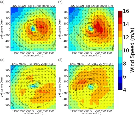
However, previous studies have not explicitly examined wind speed changes produced by the most 325
intense ECLs. Figure 1 shows the composite wind fields derived from ECLs developing near the 326
east coast of Australia (see the white rectangle in Figure SM1 in the Supplementary Material) that 327
produce maximum wind speeds of at least 20ms-1 according to the NARCliM ensemble (12 50-km 328
resolution RCM simulations). In both present and future climates, seasonal differences in the wind 329
fields are clear, with summer ECLs tending to produce higher wind speed maxima compared to 330
winter ECLs which produce a broader area of high wind speeds further from the low centre. While 331
these results agree with previous studies in terms of projecting an overall decrease in the frequency 332
of winter ECLs, they suggest no change in the frequency of the most intense and highest wind 333
producing ECLs in winter and an increase in the frequency in summer. Hence the wind hazard 334
associated with these intense events is likely to increase in the future (see the Supplementary 335
Material). 336
Further south, the overall effect of greenhouse gas forcing on ETCs during the 21st century is 337
complex because climate models indicate changes that would have opposing effects on ETC 338
activity including, for example, a reduction of the equator-to-pole temperature gradient near the 339
surface but enhanced gradients aloft (Lim and Simmonds 2009). Grieger et al. (2014) find a 340
reduction in the total number of Southern Hemisphere ETCs but an increase in the number of strong 341
ETCs particularly over the southeastern Australian region, in a multimodel ensemble of CMIP3 342
climate models. These changes are consistent with findings of a general reduction in future extreme 343
wind speed along much of the southern coastline except for Tasmania in the winter months 344
(McInnes et al. 2011). For extratropically-transitioning TCs, studies in this region of the effect of
345
climate change are currently lacking. 346
Studies have constructed scenarios of the effect of climate change on wind hazard and then applied 347
these scenarios for the estimation of future wind hazard in Australia. Wang et al. (2013) construct
348
current climate estimates of both cyclone and non-cyclone wind gust hazard in the Australian region 349
by fitting a statistical model to wind speed observations from anemometers. They then applied 350
climate change scenarios, encompassing a wide range of uncertainty and including scenarios of both 351
increases and decreases in TC intensities and frequencies, to estimate the changes in these statistical 352
distributions. For some of the scenarios that they examined, changes in wind speed return periods 353
would occur that would exceed current design standards in a number of coastal tropical locations in 354
Australia. It is noted that because of the wide range in predictions of future cyclone incidence in this 355
region, this is a highly uncertain outcome. 356
4.2 Projections of severe thunderstorm wind and hail
357
Projections of severe thunderstorm occurrence are limited: Brooks (2013) states in his recent review 358
that this question remains open. Recently, Allen et al. (2014) used an environments-based 359
approached to suggest an increase in severe thunderstorm incidence in south-east Australia, 360
although with a wide range of uncertainty. For hail, Braganza et al. (2013) reviewed this topic and 361
noted that the few available studies indicate increases in hail frequency in the southeastern regions 362
and near Sydney. 363
5. Conclusions and research gaps
364
Current hazard for various storm types has not been reliably estimated, due to either inadequate 365
length of data record or spatial gaps. These issues are particularly pronounced for hail records but 366
satellite observations have considerable potential to address these issues. The projections of future 367
wind hazard in the Australian region differ from region to region. For example, in the tropics, recent 368
evidence suggests that extreme wind hazard may decrease, although confidence in this prediction is 369
low, whereas increases are possible in the east coast region subject to ECLs. Further south, a 370
general reduction in extreme wind speed return periods may occur. All of these projections are 371
accompanied by considerable uncertainty but such uncertainty has the potential to decrease with 372
improvements in modelling techniques. 373
Identifiable research gaps vary between storm type. For TCs, while improvements have been made 374
in the confidence of projections of future wind hazard, further improvements in climate model 375
simulations of TCs are needed, through increased resolution and better representation of model 376
physics. Similar arguments can be made for ECLs. The effect of a warmer climate on extratropical 377
former TCs is a potential area of research. ETCs are better simulated because of their larger size, so 378
there the main research issue is whether the large-scale climate itself is well simulated. This issue is 379
of course important as well for all types of storms. 380
For severe thunderstorms, remote-sensing platforms offer the potential to greatly improve our 381
understanding of the associated hail and wind hazard in Australia. These include the GPATS 382
lightning-detection network (www.gpats.com.au), the new Himawari-8 satellite, and the Bureau of 383
Meteorology’s radar network, which will soon begin an upgrade to dual-polarisation. Work is 384
needed to investigate the applicability to Australian storms of existing methods of severe-weather 385
detection based on these technologies (e.g. Heinselman and Ryzhkov 2006, Schultz et al. 2009,
386
Bedka 2011). Validation of these techniques will require a large number of high-quality direct 387
observations of hail and damaging winds. Based on the success of the mPING citizen scientist 388
project in the US (Elmore et al. 2014), it is suggested that a mobile-phone application for reporting
389
severe weather would be an excellent way of obtaining these data while simultaneously engaging 390
the general public with the atmospheric science community. Reports could additionally be solicited 391
directly from the public (Ortega et al. 2009) or collected in targeted field campaigns (Heymsfield et
392
al. 2014).
394
Acknowledgements
395The authors would like to thank their respective institutions for supporting this work. J.P. Evans is 396
supported by funding from the NSW Office of Environment and Heritage funded NSW/ACT 397
Regional Climate Modelling (NARCliM) Project and the Australian Research Council as part of the 398
Future Fellowship FT110100576. 399
400
1 1
References
2
Allen JT, Allen ER (2016) A review of severe thunderstorms in Australia. Atmos Res 178-179: 3
347-366 4
Allen JT, Karoly DJ, Mills GA (2011) A severe thunderstorm climatology for Australia and
5
associated thunderstorm environments. Aust Meteorol Oceanogr J 61: 143-158
6
Allen JT, Karoly DJ (2014). A climatology of Australian severe thunderstorm environments 1979–
7
2011: interannual variability and ENSO influence. Int J Climatol 34: 81-97
8
Allen JT, Karoly DJ, Walsh KJ (2014) Future Australian severe thunderstorm environments, Part II:
9
The influence of a strongly warming climate on convective environments. J Climate 27:
10
3848-3868
11
Allen JT, Tippett MK, Sobel AH (2015) An empirical model relating U.S. monthly hail occurrence
12
to large-scale meteorological environment. J Adv Model Earth Sys 7: 226–243
13
Alexander LV, Power S (2009) Severe storms inferred from 150 years of sub-daily pressure
14
observations along Victoria's "Shipwreck Coast". Austr Meteorol Oceanogr J 58:129-133
15
Amburn SA, Wolf PL (1997) VIL Density as a hail indicator. Wea Forecast 12: 473–478
16
Bedka KM (2011) Overshooting cloud top detections using MSG SEVIRI Infrared brightness
17
temperature and their relationship to severe weather over Europe. Atmos Res 99: 175–189
18
Braganza K, Hennessy K, Alexander L, Trewin B (2013) Changes in extreme weather. In: Christoff
19
P (ed) Four Degrees of Global Warming: Australia in a Hot World, pp 33-60
20
Brooks HE (2013) Severe thunderstorms and climate change. Atmos Res 123: 129-138
21
Brooks HE, Lee JW, Craven JP (2003) The spatial distribution of severe thunderstorm and tornado
22
environments from global reanalysis data. Atmos Res 67: 73-94
23
Browning SA, Goodwin ID (2013) Large-scale influences on the evolution of winter subtropical
24
maritime cyclones affecting Australia’s east coast. Mon Wea Rev 141: 2416-2431
25
References Click here to download References 16_Walsh et
Bureau of Transport Economics (2001) Economic costs of natural disasters in Australia. Report no.
26
103, 170 pp.
27
Callaghan J, Power SB (2011) Variability and decline in the number of severe tropical cyclones
28
making land-fall over eastern Australia since the late nineteenth century. Clim Dyn 37:
647-29
662
30
Chang EK, Guo Y, Xia X (2012) CMIP5 multimodel ensemble projection of storm track change
31
under global warming. J Geophys Res Atmos 117 (D23)
32
Christensen JH et al (2013) Climate phenomena and their relevance for future regional climate
33
change. In Stocker TF et al. (eds): Climate Change 2013: The Physical Science Basis. 34
Contribution of Working Group I to the Fifth Assessment Report of the Intergovernmental
35
Panel on Climate Change (IPCC AR5) Cambridge University Press 2013, Cambridge,
36
United Kingdom and New York, NY, USA, pp 1217-1308.
37
Cintineo JL, Smith TM, Lakshmanan V, Brooks HE, Ortega KL (2012) An objective
high-38
resolution hail climatology of the contiguous United States. Wea Forecast 27: 1235–1248
39
Coles S, Bawa J, Trenner L, Dorazio P (2001). An introduction to statistical modeling of extreme
40
values (Vol. 208). London: Springer.
41
Di Luca A, Evans JP, Pepler A, et al. (2015) Resolution sensitivity of cyclone climatology over
eastern Australia using six reanalysis products. To appear in J Climate
Doswell III CA, Brooks HE, Kay MP (2005) Climatological estimates of daily local nontornadic
42
severe thunderstorm probability for the United States. Wea Forecast 20: 577-595
43
Dowdy AJ (2014) Long-term changes in Australian tropical cyclone numbers. Atmos Sci Letters
44
15: 292-298, doi:10.1002/asl2.502 45
Dowdy AJ, Kuleshov Y (2014). Climatology of lightning activity in Australia: spatial and seasonal
46
variability. Aust Meteorol Oceanogr J 6: 9-14
47
Dowdy AJ, Mills GA, Timbal B, et al (2013a) Understanding rainfall projections in relation to
Dowdy AJ, Mills GA, Timbal B (2013b) Large-scale diagnostics of extratropical cyclogenesis
in eastern Australia. Int J Climatol 33:2318–2327. doi: 10.1002/joc.3599
Dowdy AJ, Mills GA, Timbal B, Wang Y (2013c) Changes in the risk of extratropical cyclones in
eastern Australia. J Climate 26:1403–1417. doi: 10.1175/JCLI-D-12-00192.1
Evans JP, Ji F, Lee C, et al (2014) Design of a regional climate modelling projection ensemble
experiment – NARCliM. Geosci Model Dev 7:621–629. doi: 10.5194/gmd-7-621-2014
Fyfe JC (2003) Extratropical southern hemisphere cyclones: Harbingers of climate change? J
48
Climate 16:2802-2805
49
Grieger J, Leckebusch G, Donat M, Schuster M, Ulbrich U (2014) Southern Hemisphere winter
50
cyclone activity under recent and future climate conditions in multi‐model AOGCM
51
simulations. Int J Climatology 34:3400-3416
52
Hanstrum BN, Mills GA, Watson A, Monteverdi JP, Doswell III CA (2002) The cool-season
53
tornadoes of California and southern Australia. Wea Forecast 17: 705-722
54
Harper BA (1999) Numerical modelling of extreme tropical cyclone winds. J Wind Eng Industr
55
Aerodyn 83: 35-47
56
Heymsfield AJ, Giammanco IM, Wright R (2014) Terminal velocities and kinetic energies of
57
natural hailstones. Geophys Res Letters 41: 8666-8672.
58
Heinselman PL, Ryzhkov AV (2006) Validation of polarimetric hail detection. Wea Forecast 21:
59
839–850
60
Hemer MA, McInnes KL, Ranasinghe R (2013) Projections of climate change-driven variations in
61
the offshore wave climate off south eastern Australia. Int J Climatol 33:1615–1632. doi:
62
10.1002/joc.3537
63
Hemer MA, McInnes KL, Ranasinghe R (2011) Climate and variability bias adjustment of climate
64
model-derived winds for a southeast Australian dynamical wave model. Ocean Dyn 62:87–
65
104. doi: 10.1007/s10236-011-0486-4
Hermida L, Sánchez JL, López L, Berthet C, Dessens J, García-Ortega E, Merino A (2013)
67
Climatic trends in hail precipitation in France: spatial, altitudinal, and temporal variability.
68
Sci World J doi: 10.1155/2013/494971
69
Holland G, Lynch A, Leslie L (1987) Australian east-coast cyclones .1. Synoptic overview and
70
case-study. Mon Wea Rev 115:3024–3036
71
Holland GJ, Bruyere C (2014) Recent intense hurricane response to global climate change. Clim
72
Dyn 42: 617-627. doi: 10.1007/s00382-013-1713-0.
73
Holmes JD (2008 and 2011) Impact of climate change on design wind speeds in cyclonic regions.
74
JDH Consulting and Australian Building Codes Board, June 2008 and June 2011 (revised
75
edition).
76
Holmes JD, Ginger JD (2012) The gust wind speed duration in AS/NZS 1170.2, Aust J Struct Eng
77
13: 207-217
78
Hope PK, Drosdowsky W, Nicholls N (2006) Shifts in the synoptic systems influencing southwest
79
Western Australia. Clim Dyn 26:751-764
80
Hopkins LC, Holland G (1997) Australian Heavy-rain days and associated east coast cyclones:
81
1958-92. J Climatol, 10: 621-635 doi: 10.1175/1520-0442
82
Jakob D (2010) Challenges in developing a high-quality surface wind-speed data-set for Australia.
Aust Meteorol Oceanogr J 60:227-236
Ji F, Evans JP, Argueso D, et al (2015) Using large-scale diagnostic quantities to investigate change
in East Coast Lows. Clim Dyn 45: 2443-2453. doi: 10.1007/s00382-015-2481-9
JMA (2014) New geostationary meteorological satellites – Himawari-8/9. Available online at
83
http://www.jma.go.jp/jma/kishou/books/himawari/2014_Himawari89.pdf.
84
Knutson TR, Sirutis JJ, Zhao M, Tuleya RE, Bender M, Vecchi GA, Villarini G, Chavas D (2015)
85
Global projections of intense tropical cyclone activity for the late 21st century from
86
dynamical downscaling of CMIP5/RCP4.5 scenarios. J Climate 28: 7203-7224
Kossin JP, Emanuel KA, Vecchi GA (2014) The poleward migration of the location of tropical
88
cyclone maximum intensity. Nature 509: 349-352.
89
Kuleshov Y, de Hoedt G, Wright W, Brewster A (2002) Thunderstorm distribution and frequency
90
in Australia. Aust Meteorol Mag 51: 145-154
91
Kunkel KE, Karl TR, Brooks H, Kossin J, Lawrimore JH, Arndt D, Wuebbles D (2013) Monitoring
92
and understanding trends in extreme storms: State of knowledge. Bull Amer Meteorol Soc
93
94: 499-514
94
Lim E-P, Simmonds I (2009) Effect of tropospheric temperature change on the zonal mean
95
circulation and SH winter extratropical cyclones. Clim Dyn 33:19-32
96
McInnes KL, Leslie LM, McBride JL (1992) Numerical simulation of cut-off lows on the
Australian east coast: sensitivity to sea-surface temperature. Int J Climatol 12:783–795
McInnes KL, Erwin TA, Bathols JM (2011) Global Climate Model projected changes in 10 m wind
97
speed and direction due to anthropogenic climate change. Atmos Sci Letters 12:325-333.
98
doi: 10.1002/asl.341.
99
McInnes KL, Walsh KJE, Hubbert GD, Beer T (2003) Impact of sea-level rise and storm surges on
100
a coastal community. Nat Haz 30: 187-207
101
McVicar TR, Van Niel TG, Li LT, Roderick ML, Rayner DP, Ricciardulli L, Donohue R (2008).
102
Wind speed climatology and trends for Australia, 1975–2006: Capturing the stilling
103
phenomenon and comparison with near-surface reanalysis output. Geophys Res Letters, 35
104
Miller CA, Holmes JD, Henderson DJ, Ginger JD, Morrison M (2013) The response of the Dines
105
anemometer to gusts and comparisons with cup anemometers. J Atmos Ocean Tech 30:
106
1320-1336
107
Mills GA, Webb R, Davidson NE, Kepert J, Seed A, Abbs D (2010) The Pasha Bulker east coast
108
low of 8 June 2007. Centre for Australia Weather and Climate Research Tech. Rep. 23, 62
109
pp.
Oliver SE, Moriarty WW, Holmes JD (2000) A risk model for design of transmission line systems
111
against thunderstorm downburst winds. Eng Struct 22:1173-1179
112
Palutikof JP, Brabson BB, Lister DH, Adcock ST (1999) A review of methods to calculate extreme
113
wind speeds. Meteorol Appl 6:119-132
114
Pepler A, Coutts-Smith A (2013) A new, objective, database of East Coast Lows. Aust Meteorol
Oceanogr J 63:461–472
Pepler AS, Di Luca A, Ji F, et al (2014) Impact of identification method on the inferred
characteristics and variability of Australian East Coast Lows. Mon Wea Rev 143:864–877.
doi: 10.1175/MWR-D-14-00188.1
Ramsay HA, Camargo SJ, Kim D (2012) Cluster analysis of tropical cyclone tracks in the Southern
Hemisphere. Clim Dyn 39: 897-917.
Rasmussen EN, Straka JM, Davies-Jones R, Doswell III CA , Carr FH, Eilts MD, MacGorman DR
115
(1994) Verification of the origins of rotation in tornadoes experiment: VORTEX. Bull Amer
116
Meteorol Soc 75: 995–1006
117
Reinecke PA, Durran DR (2009). Initial-condition sensitivities and the predictability of downslope
118
winds. J Atmos Sci 66: 3401-341
119
Richter H (2007) A cool-season low-topped supercell tornado event near Sydney, Australia.
Preprints, 33rd Conf. on Radar Meteorology, Cairns, Australia, Amer. Meteor. Soc. and
Australian Bureau of Meteorology Research Center., P13A.16. [Available online at
https://ams.confex.com/ams/pdfpapers/123550.pdf.]
Risk Management Solutions (1999) The 1999 Sydney hailstorm: 10-year retrospective. Available at
120
http://riskinc.com/Publications/1999_Sydney_Hailstorm.pdf.
121
Sanders F, Gyakum J (1980) Synoptic-dynamic climatology of the bomb. Mon Wea Rev 108:1589–
Schultz CJ, Petersen WA, Carey LD (2009) Preliminary development and evaluation of lightning
122
jump algorithms for the real-time detection of severe weather. J Appl Meteorol Clim 48:
123
2543–2563
124
Schultz CJ, Petersen WA, Carey LD (2011) Lightning and severe weather: A comparison between 125
total and cloud-to-ground lightning trends. Wea Forecast, 26: 744-755 126
Schuster SS, Blong RJ, McAneney KJ (2005) Relationship between radar-derived hail kinetic
127
energy and damage to insured buildings for severe hailstorms in Eastern Australia. Atmos
128
Res 81: 215–235
129
Schuster SS, Blong RJ, Speer MS (2006) A hail climatology of the Greater Sydney area and New
130
South Wales, Australia. Int J Clim 25: 1633–1650
131
Sinclair MR (2002) Extratropical transition of southwest Pacific tropical cyclones. Part I:
132
climatology and mean structure changes. Mon Weather Rev 130: 590–609
133
Soderholm J, McGowan H, Richter H, Walsh K, Weckwerth T, Coleman M (2015) The Coastal
134
Convective Interactions Experiment (CCIE): Understanding the role of sea breezes in
135
climatological hailstorm hotspots in Eastern Australia. Submitted to Bull Amer Meteorol
136
Soc
137
Speer M, Wiles P, Pepler A (2009) Low pressure systems off the New South Wales coast and
associated hazardous weather: establishment of a database. Aust Meteorol Oceanogr J
58:29–39
Standards Australia (2011) Structural design actions. Part 2: Wind actions, Australian/New Zealand
138
Standard, AS/NZS 1170.2:2011, Standards Australia, Sydney, NSW.
139
Strachan J, Vidale PL, Hodges K, Roberts M, Demory M-E (2013) Investigating global tropical
140
cyclone activity with a hierarchy of AGCMs: the role of model resolution. J Climate 26:
141
133-152, doi: 10.1175/JCLI-D-12-00012.1.
142
Troccoli A, Muller K, Coppin P, Davy R, Russell C, Hirsch AL ( 2012) Long-term wind speed
143
trends over Australia. J Climate 25: 170–183
Walsh KJE, Camargo SJ, Vecchi GA, et al. (2015) Hurricanes and climate: the U.S. CLIVAR 145
working group on hurricanes. Bull Amer Meteorol Soc 96: 997-1017
146
Wang CH, Wang X, Khoo YB (2013) Extreme wind gust hazard in Australia and its sensitivity to
147
climate change. Nat Haz 67: 549-567
148
Witt A, Eilts MD, Stumpf GJ, Johnson JT, Mitchell ED, Thomas KW (1998) An enhanced hail
149
detection algorithm for the WSR-88D. Wea Forecast 13: 386–303
150
Wurman W, Dowell D, Richardson Y, Markowski P, Rasmussen E, Burgess D, Wicker L, Bluestein
151
HB (2012) The second Verification of the Origins of Rotation in Tornadoes Experiment:
152
VORTEX2. Bull Amer Meteorol Soc 93: 1147-1170
1
1
Figure 1: Ensemble composites of summer (DJF: top row) and winter (JJA: bottom row) ECLs
2
with a maximum wind speed greater than 20ms-1 from the NARCliM ensemble for the recent past
3
(1990-2010: left column) and the future (2060-2079: right column). Coloured contours and vectors 4
indicate wind speed while solid line contours indicate the sea level pressure. The ensemble-mean 5
number of events within the composite is indicated to the top-right of each panel. 6
7
[image:27.595.58.532.58.465.2]