Evolutionary models in structured populations

(1)

City, University of London Institutional Repository

Citation

:

Hadjichrysanthou, C. (2012). Evolutionary models in structured populations. (Unpublished Doctoral thesis, City University London)

This is the unspecified version of the paper.

This version of the publication may differ from the final published

version.

Permanent repository link: http://openaccess.city.ac.uk/1731/

Link to published version

:

Copyright and reuse:

City Research Online aims to make research

outputs of City, University of London available to a wider audience.

Copyright and Moral Rights remain with the author(s) and/or copyright

holders. URLs from City Research Online may be freely distributed and

linked to.

City Research Online: http://openaccess.city.ac.uk/ [email protected]

(2)

EVOLUTIONARY MODELS

IN

STRUCTURED POPULATIONS

Christoforos C. Hadjichrysanthou

Thesis submitted to City University London

for the degree of Doctor of Philosophy

City University London

School of Engineering and Mathematical Sciences

Centre for Mathematical Science

(3)

(4)

List of Figures

1.1 The Moran process with frequency dependent fitness . . . 14

1.2 A spatial evolutionary game . . . 19

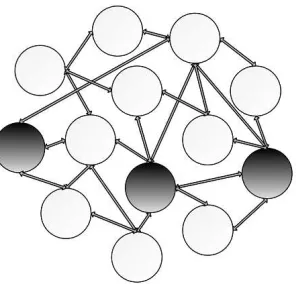
1.3 A population represented by a graph . . . 20

2.1 Structured populations represented by graphs: a complete graph, a

circle graph and a star graph . . . 34

2.2 Comparison of the average fixation probability of a single mutant on

a star graph under the rules of the IP, with the fixation probability in

the Moran process, in the constant fitness case . . . 58

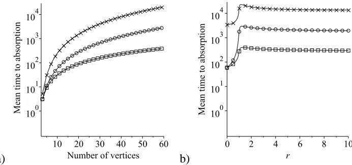
2.3 Comparison of the mean time to absorption starting from a single

mutant on a star graph, a circle and a complete graph under the rules of the IP, in the constant fitness case . . . 59

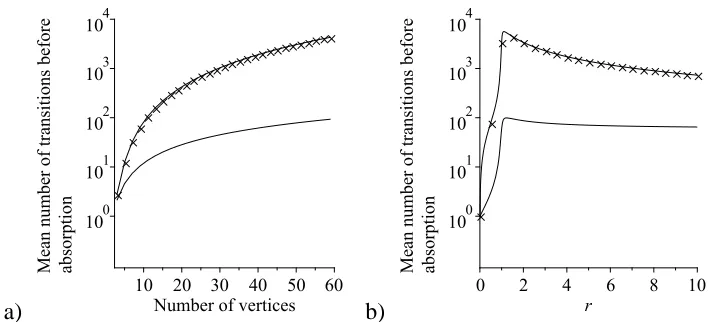
2.4 Comparison of the mean number of transitions until absorption

start-ing from a sstart-ingle mutant on a star graph under the rules of the IP,

with the mean number of transitions in the Moran process, in the

constant fitness case . . . 61

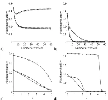
2.5 Comparison of the average fixation probability of a single mutant

Hawk on a star graph, a circle and a complete graph under the rules

of the IP, in a Hawk–Dove game . . . 63

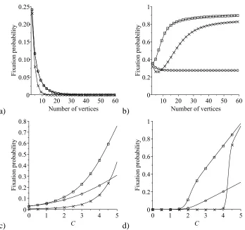
2.6 Comparison of the average fixation probability of a single mutant

Dove on a star graph, a circle and a complete graph under the rules

of the IP, in a Hawk–Dove game . . . 65

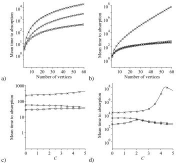
2.7 Comparison of the mean time to absorption starting from a single mutant Hawk on a star graph, a circle and a complete graph under

the rules of the IP, in a Hawk–Dove game . . . 66

2.8 Comparison of the mean time to absorption starting from a single

mutant Dove on a star graph, a circle and a complete graph under

(9)

List of Figures

start-ing from a sstart-ingle mutant Hawk on a star graph, a circle and a

com-plete graph under the rules of the IP, in a Hawk–Dove game . . . 68

start-ing from a sstart-ingle mutant Dove on a star graph, a circle and a

com-plete graph under the rules of the IP, in a Hawk–Dove game . . . 69

3.1 The fixation probability of Hawks and the mean time to absorption, starting from a single mutant Hawk on a complete graph under the

IP, the BD-D process, the VM and the DB-B process, in a Hawk–

Dove game . . . 79

3.2 The average fixation probability of a single mutant on a star graph

under the IP, the BD-D process, the VM and the DB-B process, in

the constant fitness case . . . 82

3.3 The behaviour of r1(n), r2(n), r3(n), r4(n), r5(n) and r6(n), as n

increases . . . 85

3.4 The mean time to absorption starting from a single mutant on a star

graph under the IP, the BD-D process, the VM and the DB-B

pro-cess, in the constant fitness case . . . 85

3.5 The mean fixation time of a single mutant on a star graph under the IP, the BD-D process, the VM and the DB-B process, in the constant

fitness case . . . 86

3.6 The average fixation probability of a single mutant Hawk on a star

graph under the IP, the BD-D process, the VM and the DB-B

pro-cess, in a Hawk–Dove game . . . 88

3.7 The mean time to absorption starting from a single mutant Hawk on

a star graph under the IP, the BD-D process, the VM and the DB-B

process, in a Hawk–Dove game . . . 89

3.8 The average fixation probability of a single mutant cooperator on a

star graph under the IP, the BD-D process, the VM and the DB-B

process, in a Prisoner’s Dilemma game . . . 91

3.9 The average fixation probability of a single mutant playing strategy A on a star graph under the IP, the BD-D process, the VM and the

DB-B process, in a coordination game . . . 92

4.1 Diagram showing all the probabilities of transition from and to the

classes Mm,r and Rm,r . . . 105

(10)

List of Figures

4.2 Change over time in the proportion of individuals playing the Hawk

strategy in a Hawk–Dove game played on a random regular graph, a

random graph and a scale-free network. The solution of the

Neigh-bourhood Configuration model, the solution of the pairwise model

and the average of 100 stochastic simulations are presented . . . 107

4.3 The proportion of Hawks in the equilibrium on random graphs of

different average degree. The solution of the Neighbourhood Con-figuration model, the solution of the pairwise model and the average

of 100 stochastic simulations are presented . . . 108

5.1 Change over time in the density of searchers, handlers and

fight-ers on a random regular graph. The respective solution in the

well-mixed population is also presented . . . 118

5.2 The equilibrium density of searchers, handlers and fighters, and the

equilibrium density of the pairs F−F and Fj−Fj, on random

regu-lar graphs of different degree . . . 118

5.3 The equilibrium density of searchers, handlers and fighters, and the

equilibrium density of the pairs F−F and S−F, on a random

reg-ular graph as the clustering coefficient varies . . . 120 5.4 Change over time in the density of searchers, handlers and fighters

on a random graph. The respective solution in the well-mixed

pop-ulation is also presented . . . 121

5.5 Change over time in the density of searchers, handlers and fighters

on a scale-free network. The respective solution in the well-mixed

population is also presented . . . 121

6.1 Schematic representation of all the possible events that might

hap-pen until the consumption of a food item by a mutant searcher

play-ing strategy (q1,q2,q3) who encounters a handler of a population

playing strategy(p1,p2,p3). The transition probabilities and the ex-pected times to move from one state to another are shown . . . 135

6.2 Schematic representation of all the possible events that might

hap-pen until the consumption of a food item by a mutant handler

play-ing strategy (q1,q2,q3) who encounters a searcher of a population

playing strategy(p1,p2,p3). The transition probabilities and the

(11)

List of Figures

6.3 Graphs showing examples of the region where each of the four

pos-sible ESSs (Retaliator, Marauder, Attacking Sharer and Hawk) is an

ESS as the duration of the content and the handling time of a sharer

vary . . . 142

6.4 Graphs showing examples of the region where each of the four

pos-sible ESSs (Retaliator, Marauder, Attacking Sharer and Hawk) is an

ESS as the density of the population and the rate at which foragers find undiscovered food vary . . . 143

6.5 A graph showing an example of the region where each of the three

possible ESSs (Retaliator, Attacking Sharer and Hawk) can occur in

the special case where 2tc=th, as the probability of the challenger

winning and the duration of the content vary . . . 146

C.1 The expected time until the consumption of a food item of searcher

animals playing strategies (1,1,0), (0,1,0) and (0< p1 <1,1,0)

in a population playing strategy(0<p1<1,1,0), and the expected

time until the consumption of a food item of handler animals playing

strategies(0.8,1,0),(0.8,0,0)and(0.8,0< p2<1,0)in a popula-tion playing strategy(0.8,0< p2<1,0) . . . 178

(12)

List of Tables

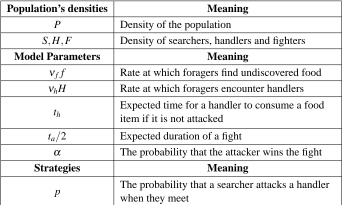
1.1 Notation of the basic game-theoretical model of kleptoparasitism of

Broom and Ruxton (1998) . . . 25

3.1 Comparison of the average fixation probability and the mean times

to absorption and fixation of a single mutant on a star graph in the

constant fitness case between the IP, the BD-D process, the VM and

the DB-B process . . . 84

5.1 The equilibrium proportion of searchers, handlers and fighters that

occupy vertices of different degree in a scale-free network . . . 122

6.1 Notation of the game-theoretical model of food sharing in

kleptopar-asitic populations . . . 130

6.2 Notation of the required times to the consumption of a food item

from the different foraging states . . . 134

6.3 Conditions under which a mutant playing strategy(q1,q2,q3)cannot

invade a population playing strategy(p1,p2,p3) . . . 140

6.4 Conditions under which a mutant playing strategy(q1,q2,q3)cannot

invade a population playing strategy(p1,p2,p3) in the special case

where 2tc=th . . . 147

C.1 Possible ESSs in the game-theoretical model of food sharing in

(13)

(14)

Acknowledgments

I firstly wish to express my deepest gratitude towards my thesis advisor,

Profes-sor Mark Broom. His perceptive and substantial advices were determinants of the

smoothness and the progression of my research work. His professionalism,

knowl-edge and experience in combination with his character, approachability, acumen and

willingness to help are the main qualities of the ideal research advisor. I am really

honoured to have worked with him.

I am especially thankful to my collaborator Dr Istvan Z. Kiss, the person whose

contribution in laying the foundations of my research career was of major

impor-tance. His ideas, valuable guidance and suggestions were crucial for the derivation of key results of this work. His enthusiasm, goodwill and readiness to help at any

time are really appreciated.

I would also like to acknowledge my collaborator Dr Jan Rycht´aˇr. Our great

col-laborative relationship, his assistance and helpful advises resulted in the successful

completion of a number of projects included in this research work.

I am sincerely grateful to the Engineering and Physical Sciences Research

Coun-cil (EPSRC), the University of Sussex and the City University London for providing

scholarships and facilities to undertake this course of study.

I could not take this opportunity to thank my parents. Their unconditional love

and financial and emotional support during my studies, and in general in my life,

their patience, their unwavering faith in me and continuous encouragement have enabled me to set and achieve targets.

Last but not least, I would like to thank my little “kattith”, Elena Iacovidou, the

person that was next to me in every single moment throughout this course,

(15)

(16)

Declaration

This thesis is entirely my own work, except where otherwise indicated.

This thesis is submitted to City University London for the Degree of Doctor of

Philosophy, and no part of the work included in this thesis has been submitted in

(17)

(18)

Abstract

Evolutionary dynamics have been traditionally studied in infinitely large homo-geneous populations where each individual is equally likely to interact with every other individual. However, real populations are finite and characterised by com-plex interactions among individuals. In this work, the influence of the population structure on the outcome of the evolutionary process is explored.

Through an analytic approach, this study first examines the stochastic evolution-ary game dynamics following the update rules of the invasion process, an adaptation of the Moran process, on finite populations represented by three simple graphs; the complete graph, the circle and the star graph. The exact formulae for the fixation probability and the speed of the evolutionary process under different conditions are derived, and the effect of the population structure on each of these quantities is stud-ied.

The research then considers to what extent the change of the strategy update rules of the evolutionary dynamics can affect the evolutionary process in structured populations compared to the process in homogeneous well-mixed populations. As an example, the evolutionary game dynamics on the extreme heterogeneous structure of the star graph is studied analytically under different update rules. It is shown that in contrast to homogeneous populations, the choice of the update rules might be crucial for the evolution of a non-homogeneous population.

Although an analytic investigation of the process is possible when the contact structure of the population has a simple form, this is usually infeasible on complex structures and the use of various assumptions and approximations is necessary. This work introduces an effective method for the approximation of the evolutionary pro-cess in populations with a complex structure.

Another component of this research work involves the use of game theory for the modelling of a very common phenomenon in the natural world. The models de-veloped examine the evolution of kleptoparasitic populations, foraging populations in which animals can steal the prey from other animals for their survival. A basic game-theoretical model of kleptoparasitism in an infinite homogeneous well-mixed population is extended to structured populations represented by different graphs. The features of the population structure that might favour the appearance of klep-toparasitic behaviour among animals are addressed.

(19)

(20)

CHAPTER 1 Introduction

Evolution of populations has been an issue of great concern in the last centuries.

Although evolution is a broad term, one can simply define it as a process by which

populations change in the heritable characteristics over time. There have been

vari-ous theories proposed in order to explain evolutionary changes in populations. In the middle of the 19th century, Charles Darwin published a book, entitled ‘On the

Ori-gin of Species by Means of Natural Selection’, suggesting a revolutionary theory to

explain evolution. Populations evolve by natural selection. Individuals occasionally

mutate. Mutation is a genetic change due to an error in the reproduction process.

These alterations generate differences among individuals in their ability to survive

and reproduce. If the new individuals have a survival and reproductive advantage in

their environment, then they reproduce at higher rates passing on their

characteris-tics to their offspring. Disadvantageous individuals have a lower chance of survival

and reproductive success and thus they are more likely to die out over time. Neutral mutant individuals, i.e. mutants that are neutral with respect to natural selection,

might incorporate into the population by neutral drift. Natural selection acts on

in-dividuals, but only the population of individuals evolves over time. The time needed

for a population to evolve depends on the nature of the population and might vary

from minutes to millions of years. A population might be a human population, an

animal population, a population of cells, multicellular organisms, molecules such as

DNA and proteins, or any other evolving population. An outgrowth of Darwinian

evolution is the cultural evolution which refers to cultural and social changes that

occur over time (for example an erroneous imitation of behavioural traits, changes

in the human language, ideas and opinions, strategic choices etc.).

Evolutionary game theory has been proven to be a powerful mathematical tool

for the description and the study of the evolution of populations consisting of

(21)

Introduction

the evolution of virulence in host-parasite interactions, the evolution of opinions

through social interactions, and the evolution of populations of animals competing

either over territory, mates, food or other biological resources, or for social status,

using different strategies.

This chapter is an introductory chapter in game theory and evolutionary graph

theory. It introduces the basic concepts of the classical and evolutionary game

the-ory and some of the fundamental tools for the study of evolutionary game dynamics in finite homogeneous well-mixed populations of constant size through a

stochas-tic approach. The famous Moran process is described and important quantities in

the stochastic evolutionary process are considered. Then, evolutionary dynamics in

structured populations and the basic idea of studying evolution of populations

rep-resented by graphs are discussed. Applications of game theory in the modelling of

kleptoparasitism are also presented. At the end, the contributions and the outline of

this work are provided.

1.1 Classical game theory

Game theory is the study of strategic decision-making of individuals. Game

the-ory has a long histthe-ory with origin in the 1920s when John von Neumann published

a series of papers (summarised later in the book von Neumann and Morgenstern

(1944)), although discussions of game theory had started much earlier, at the

be-ginning of the 18th century. It has been applied to study individuals’ behaviour in

decision making problems in a wide variety of fields, including economics, biology,

ecology, computer science, sociology, psychology and political sciences.

A strategic game is a model of interacting decision-makers, the players. At each

stage of the game, each of the players has to take an action. The player’s strategy

determines the action taken at every possible stage of the game. Each player has a preference relation on the set of action profiles, which is represented by the

so-called payoffs, i.e. the payoffs define a preference ordering. In other words, a payoff

represents the motivation of a player to choose a specific strategy, the “award” of a

choice. The payoff of each player might be affected not only by its own action but

also by the action chosen by the other players that it is interacting with. In each case,

the players try to attain the maximum possible payoff by choosing an appropriate

action. The players might use pure strategies or mixed strategies. A pure strategy

defines a specific action that a player will take at every possible stage of the game.

The number of pure strategies can be either finite or infinite. A mixed strategy is a strategy according to which a player uses each of the available pure strategies

(22)

Introduction

with a certain probability. Since a probability can be any real number between 0

and 1, there is an infinite number of mixed strategies. A mixed strategy is usually

represented by a row vector (probability vector) whose ith entry is the probability

that a player uses the ithavailable pure strategy.

Depending on the nature of the strategic game, there are different ways to

de-scribe it. A commonly known type of game is the game in normal form (or strategic

form). Games in this form consist of a finite number of players, a set of pure strate-gies available for each player to use, and the payoff function which determines the

payoff of each player depending on its strategy and the strategy of its opponents.

In normal form games all individuals play a strategy simultaneously, or individuals

are not aware of the strategy of their opponents. When there are just two players

and the number of available strategies for each player is finite, the game is usually

called a Bimatrix game. In such games, the outcome of the payoff function can be

represented by a matrix, the so-called payoff matrix. Assume two players, Player 1

and Player 2, where Player 1 has a finite strategy set S={S1, . . . ,Sm}and Player 2

a finite strategy set T ={T1, . . . ,Tn}. The column of the payoff matrix represents

the strategic choices of the one player and the row the strategic choices of the other.

Each element in row i and column j of the matrix is an ordered pair(si,tj), where

si represents the payoff received by the “row player” and tj the payoff received by

the “column player” when the row player plays strategy Si and the column player

plays strategy Tj. For every possible combination of pure strategies Si, i∈[1,m],

and Tj, j∈[1,n], there is a corresponding pair of numbers(si,tj). This game can be

represented by the following payoff matrix

Player 2 (Column Player)

Strategy T1 . . . Tj . . . Tn

S1 (s1,t1) . . . (s1,tj) . . . (s1,tn)

Player 1 ... ... . . . ... . . . ...

(Row Player) Si (si,t1) . . . (si,tj) . . . (si,tn)

..

. ... . . . ... . . . ...

Sm (sm,t1) . . . (sm,tj) . . . (sm,tn)

. (1.1)

In the case of symmetric games, i.e. games where both players have the same

strategic choices, S={S1. . .Sn}, and the payoff obtained by using each strategy is

irrespective of the player that uses it, the game can be described by a square n×n

payoff matrix, whose element in the ithrow and jth column represents the payoff of

(23)

Introduction

For example, in a two-player symmetric game in normal form where there are two

possible strategies for each player, A and B (such games are also called 2×2 games), the interactions between the individuals can be described by the payoff matrix

A B

A a b

B c d

. (1.2)

An individual playing strategy A (A individual) obtains a payoff a when interacting

with another individual playing A and a payoff b when interacting with an individual

playing B (B individual). Similarly, an individual playing strategy B obtains payoffs

c and d when interacting with an individual playing A and an individual playing B,

respectively.

In this work, we will consider two-player symmetric games in normal form.

1.1.1 Dominant strategies and Nash equilibria

In this section, we present in a simple way some important definitions and main

solution concepts of the classical game theory.

The best response strategy is the strategy (or strategies) that when it is used

against a given strategy offers the highest possible payoff. If this strategy is unique,

i.e. it results in a strictly higher payoff against a given strategy then it is called the

strict best response to that strategy.

A dominant strategy (strictly dominant strategy) is a strategy that is a (strict) best response to every other strategy, i.e. it results in the highest payoff compared to the

other available strategies no matter what the opponent does.

A Nash equilibrium (Nash, 1951) is a set of strategies consisting of a strategy

for each player. The strategy of each player is a best response to the other players’

strategy, i.e. if any of the players chooses a different strategy and the strategies

of the other players remain unchanged, its payoff will either remain the same or

decrease. If the decrease in payoff is the only possible result of such a choice, then

the set of strategies is called a strict Nash equilibrium. If a player has a strictly

dominant strategy, then this strategy is obviously the one that is used in the Nash

equilibria of the game. In mathematical terms, in a two-player symmetric game, a strategy i is a Nash equilibrium if E(i,i)≥E(j,i)∀j, and a strict Nash equilibrium

if E(i,i)>E(j,i)∀j6=i, where E(X,Y) represents the payoff for playing strategy X against strategy Y. A game can have either a pure-strategy or a mixed-strategy

Nash equilibrium. Although in general pure strategy Nash equilibria may not exist,

(24)

Introduction

it is proved (Nash, 1951) that in a finite game (a game that has a finite number of

players and actions) there always exists a Nash equilibrium if individuals can use

mixed strategies.

Two concepts which are sometimes important are those of Pareto efficiency and

risk-dominance. A strategy is called Pareto efficient (or Pareto optimal) if there is

no any other strategy that can improve the payoff of a player without reducing the

payoff of at least one other player. Note that a Nash equilibrium is not necessarily Pareto efficient; there might be sets of strategies which may result in better outcomes

for both players but are not Nash equilibria. A strategy is called risk dominant if it

has the largest basin of attraction, i.e. it becomes more preferable in cases where the

uncertainty about the strategy of the opponents increases. For example, in a 2×2 game described by the payoff matrix (1.2) where strategies A and B are strict Nash

equilibria, i.e. a>c and b<d, if a>d then A is Pareto efficient, but if a+b<c+d

then B is risk-dominant, given that each player assigns probability 0.5 to each of

the strategies A and B. It is often interesting to consider when selection favours

the Pareto efficient Nash equilibrium over the risk dominant Nash equilibrium, for example in coordination games (see Sections 1.3.3 and 3.4.2).

1.2 Evolutionary game theory

In contrast to the classical game theory where individuals play a static game and

choose the strategy that offers them the maximum possible payoff, given that all

individuals behave rationally, evolutionary game theory is a dynamic theory which

studies the evolution of populations where individuals interact repeatedly with other

individuals. The different strategies might be thought of as different types of

in-dividuals and the payoffs obtained by each individual when interacting with other individuals are interpreted as fitness, which determines the reproductive and survival

success. Therefore, depending on the payoff values, the fitness of each individual

might be either constant (constant fitness) or dependent on the frequency (relative

proportion) of the other types of individuals in the population (frequency dependent

fitness).

The evolutionary process is mainly determined by the selection and mutation

process. In terms of the evolutionary game theory, under selection individuals with

the highest payoff (and thus fitness) are more likely to pass on their traits (genetic or

cultural) to subsequent generations. Consequently, the frequency of these

(25)

Introduction

subsequent generations.

Evolutionary game dynamics have been traditionally studied in infinitely large

unstructured populations where every individual is equally likely to meet every other

individual. There are two traditional approaches to evolutionary game theory. The

first is the approach of Maynard Smith and Price (1973) who introduced the concept

of an Evolutionarily Stable Strategy. The second approach studies the variation in

the frequency of the different types of individuals over time through the construction of a dynamical system of equations, the replicator equations.

1.2.1 Evolutionarily Stable Strategies

A strategy is an Evolutionarily Stable Strategy (ESS) (Maynard Smith and Price,

1973) if a population adopting that strategy cannot be invaded by a small number

of individuals playing any alternative strategy (mutant strategy), i.e. if it is stable

with respect to changes in strategic choices of individuals. But let us consider the

definition of an ESS in mathematical terms.

Consider an infinitely large resident population where all individuals use a

strat-egy (pure or mixed), R. Assume that initially all individuals have a background

(initial) fitness equal to fb and let∆f(X,Y)be the change in fitness for an

individ-ual of a subpopulation that plays strategy X (X individindivid-ual) when interacting with an

individual of a subpopulation that plays strategy Y (Y individual) (this is equal to

the payoff of an X individual when playing against a Y individual). The expected

fitness of an individual of a population where all individuals use strategy R, is

fR= fb+∆f(R,R). (1.3)

Assume that this population is invaded by a very small proportionε of mutant

viduals that play strategy M. In this case, the expected fitness of a random R

indi-vidual of the population is given by

fR= fb+ (1−ε)∆f(R,R) +ε∆f(R,M), (1.4)

and the expected fitness of a random individual playing the mutant strategy is

fM= fb+ (1−ε)∆f(M,R) +ε∆f(M,M). (1.5)

Mutant individuals playing strategy M cannot invade a population of individuals

playing strategy R, if

fR> fM, (1.6)

(26)

Introduction

for all the possible strategies M6=R. Since ε is a very small proportion close to zero, this is true if

∆f(R,R)>∆f(M,R)or (1.7)

∆f(R,R) =∆f(M,R)and∆f(R,M)>∆f(M,M). (1.8)

A strategy R is an ESS if either the condition (1.7) or the condition (1.8) holds for all

the available strategies M, M6=R. In words, the condition (1.7) means that a very small proportion of mutant individuals playing strategy M cannot invade a

popula-tion of resident individuals playing R if an individual playing strategy R compared

with an individual playing strategy M has an advantage when both play against an

individual that plays R, i.e. if R is a strict best response to itself. The condition (1.8)

means that even if a resident individual does equally well with a mutant when

play-ing against a resident, the mutants cannot invade the population as long as a resident

does better when playing against a mutant, i.e. if R is a better response to M, than

M to itself.

It follows from conditions (1.7) and (1.8) that a necessary condition for a

strat-egy to be an ESS is for it to be a Nash equilibrium, and thus every ESS is a Nash equilibrium. But note that a Nash equilibrium is not necessarily an ESS. If a

strat-egy is a strict Nash equilibrium, then condition (1.7) must hold, and thus every strict

Nash equilibrium is an ESS.

It should be noted that there might be conditions under which there are many

possible ESSs simultaneously and the population stabilised into one of these. On

the other hand, there might be circumstances in which there are no ESSs.

A limitation of the evolutionarily stable strategy concept is that it begins from

the state in which all the members of the population play the same strategy

with-out considering how this state has been reached. In addition, it considers only the

stability of the population strategy in isolated changes in the strategic choices of a

very small proportion of the population, without considering any mutations during the evolutionary process. Furthermore, the concept holds as long as the population

size is infinite, and population structure and stochasticity are ignored.

1.2.2 Replicator Dynamics

In contrast to the concept of evolutionarily stable strategies, the replicator dynamics

describe how the frequencies of strategies within a population change in time.

Consider a homogeneous well-mixed population of infinite size where

(27)

Introduction

simplest case where individuals can use either strategy A or strategy B. The game

played between the individuals is described by the payoff matrix (1.2). The expected

fitnesses of individuals playing strategy A and B are given respectively by

fA= fb+xAa+xBb, (1.9)

fB= fb+xAc+xBd. (1.10)

xA is the frequency of individuals playing strategy A, and xB the frequency of

indi-viduals playing B. The average fitness of the population is thus given by

F =xAfA+xBfB. (1.11)

Since the population consists only of individuals that play either strategy A or

strat-egy B, xA+xB=1. The evolution of the population can be described by the

follow-ing dynamic equation,

˙

xA=xA(fA−F). (1.12)

This is called the replicator equation (Taylor and Jonker, 1978; Hofbauer et al.,

1979; Hofbauer and Sigmund, 1998, 2003).

From equation (1.12), it is obvious that at any time, if the fitness of individuals

playing A is higher than the average fitness of the population, their frequency will

increase. If their fitness is lower than the average fitness of the population, then their

frequency will decrease. Hence, the replicator equation describes the deterministic

selection process where more successful strategies spread in the population. As in

the approach discussed in the previous section, mutation is not considered.

Substituting equations (1.9)–(1.11) into (1.12) we obtain

˙

xA=xA(1−xA)(fA−fB) (1.13)

=xA(1−xA) xA(a−b−c+d) +b−d

. (1.14)

From (1.14) we see that there are three generic equilibrium points,

x∗_A=0, (1.15)

x∗_A=1, (1.16)

x∗_A= b−d

b+c−a−d, for a>c and b<d, or for a<c and b>d. (1.17)

Note that as in the ESS concept, the background fitness of individuals is irrelevant and only the values of the payoffs matter.

(28)

Introduction

There are three distinct generic scenarios for the evolutionary process:

i. Dominance: In this case, either strategy A is always better no matter what the

opponent does and thus the equilibrium point x∗_A =1 is stable (the case where

a>c and b>d), or B is always better than A and thus the equilibrium point

x∗_A =0 is stable (the case where a<c and b <d). In each case, the better

strategy is a strict Nash equilibrium and therefore an ESS.

ii. Bistability: The two equilibrium points x∗_A=0 and x∗_A=1 are both strict Nash equilibria, and thus strategies A and B are both ESSs. The equilibrium point

given by (1.17) is unstable. Evolution will result in the fixation of As when their

frequency is above x_A∗, and in their extinction when their frequency is below x∗_A. This is the case where a>c and b<d.

iii. Coexistence: The interior equilibrium point (1.17) is stable while the points

x∗_A=0 and x∗_A=1 are both unstable. This is the case where a<c and b>d.

In the non-generic cases where a≥c and b>d, or a>c and b≥d, strategy A

also dominates B. In the cases where a≤c and b<d, or a<c and b≤d, B also

dominates A.

In the non-generic case where a=c and b=d, i.e. fA = fB for all values of

xA, the two strategies do equally well and thus the frequency distribution of the

strategies remains constant. This case is called the neutral case. Although this case

is not much of interest in the replicator dynamics, as we will see in Chapters 2 and

3, it is an interesting and important case in the stochastic evolutionary dynamics of

finite populations.

Note that constant selection, where individuals have constant fitness indepen-dent of the interactions with other individuals and thus of the composition of the

population, can be obtained in the special case where a=b and c=d.

The replicator equation can be generalised for n different strategic types of

indi-viduals. Consider a population where each individual interacts in equal likelihood

with any other individual and can use one of the n available pure strategies of the set

S. The change of the frequencies xi, i∈[1,n], of the different types of individuals

over time is described by the equations

˙

xi=xi(fi−F), (1.18)

where fiis the expected fitness of an individual that uses strategy Siand is given by

fi= fb+∑nj=1xj∆f(Si,Sj), and F is the average fitness of the entire population and

(29)

Introduction

1.3 Some classical games

In this section, we present some of the classical games that have been widely studied

and applied in different fields.

1.3.1 The Hawk–Dove game

The Hawk–Dove game (Maynard Smith and Price, 1973; Maynard Smith, 1982) is

possibly the most classic evolutionary game. This game has been used extensively

for the modelling of competition of animals over food, mates, territories, and other

biological resources. According to this game, individuals interact with each other

over a resource of value V by playing either aggressively using the Hawk

strat-egy (H) or non-aggressively using the Dove stratstrat-egy (D). If two individuals playing

Hawk meet, a fight takes place. At the end of the fight, the winner of the game gets

a payoff V while the loser pays a cost C. Therefore, the two players obtain a payoff on average equal to(V−C)/2. If two Doves meet, they either equally share the resource (if divisible) or with equal probability one of the two takes the whole

re-source with no cost. Thus, in this case Doves obtain an average payoff equal to V/2.

If a Hawk meets a Dove, the Dove retreats leaving the resource to the Hawk without

any cost, and thus the Hawk obtains a payoff, V , while the Dove gets nothing. This

game is described by the following payoff matrix:

H D

H a=V−₂C b=V

D c=0 d=V₂

. (1.19)

It is clear that since b>d, the Dove strategy is never evolutionarily stable because a

population of Doves can always be invaded by a Hawk. If the value of the resource

outweighs the cost of the fight, i.e. if V >C ⇒a>c, since b>d, an individual

always does better by playing the Hawk strategy no matter what the opponent does (the Hawk strategy is strictly dominant). Thus, in an infinite homogeneous

well-mixed population the Hawk strategy is the unique pure ESS. Hawk is also the unique

pure ESS when V =C, because b>d. If V <C⇒a<c, it is better to play Dove

when Hawks are common. Since it is better to play Hawk when Doves are common,

this leads to an evolutionarily stable mixed strategy. Assume that with probability

p∈(0,1)individuals use the Hawk strategy, and with probability 1−p they use the

Dove strategy. In order a mixed strategy(p∗,1−p∗)to be an ESS, in a population playing strategy(p∗,1−p∗), the fitness of an individual playing the Hawk strategy

(30)

Introduction

must be equal to the fitness of an individual playing the Dove strategy, i.e.

p∗V−C

2 + (1−p

∗₎_V ₌_p∗₀_{+ (}₁₋_p∗₎V

2. (1.20)

Solving for p∗we obtain that p∗=V/C. It is easy to show that an individual playing

the mixed strategy(V/C,1−V/C)in a population playing any other strategy(p,1−

p), p∈ [0,1], has a higher fitness than an individual of that population. Hence, according to condition (1.8), there is a unique mixed ESS where individuals play

Hawk with probability V/C and Dove with probability 1−V/C. The mixed ESS

can also be found by using the approach in Section 1.2.2.

Note that here we assumed a monomorphic population where all individuals

choose randomly between the pure strategies according to a given probability

dis-tribution, and thus all individuals play the same mixed strategy. A similar method

could be followed in the case of a polymorphic population where individuals use

dif-ferent pure strategies. In this case, the mixture of strategies is a polymorphic mixture

of individuals where a proportion of the population equal to V/C uses the pure Hawk

strategy and a proportion 1−V/C uses the pure Dove strategy. Mathematically, in

infinite unstructured populations, the two cases are equivalent because in either case

an individual of the population has a probability p of meeting an individual playing Hawk and a probability 1−p of meeting an individual playing Dove.

1.3.2 The Prisoner’s Dilemma game

The Prisoner’s Dilemma (Axelrod, 1984; Poundstone, 1992) is one of the most

pop-ular games in game theory and has been commonly applied for the study of the

evolution of cooperation.

Assume a population where individuals either cooperate (use strategy C) or

de-fect (use strategy D). Mutual cooperation results in a payoff R (reward) while mutual defection results in a payoff P (punishment). T (temptation) is the payoff obtained

by a defector against a cooperator and S (sucker’s payoff) is the payoff of a

cooper-ator against a defector. The game is described by the payoff matrix

C D

C R S

D T P

. (1.21)

In the Prisoner’s Dilemma, the order of the elements of the payoff matrix (1.21)

is T >R>P>S. Thus, in this game, mutual cooperation results in a higher payoff

(31)

Introduction

a population of all defectors. However, since T >R and P>S, it is always better

to defect regardless of what the partner does and thus mutual defection is the unique

Nash equilibrium, and defection is the only ESS.

In its simplest form, the Prisoner’s Dilemma can be described as the game where

a cooperator provides a benefit B to its partner at a cost C to itself. A defector just

receives the benefit from a cooperator without paying any cost. The payoff matrix

of the game in this form is

C D

C B−C −C

D B 0

, (1.22)

with B>C>0.

1.3.3 Coordination games

A coordination game is a game with multiple pure strategy Nash equilibria. In

a two strategy game described by the payoff matrix (1.2), a coordination game is

defined by a>c and b<d, and thus strategies A and B are both Nash equilibria.

The replicator dynamics also predicts an unstable interior equilibrium where the

population fraction of A individuals, x∗_A, is given by (1.17). Usually, one of the strategies in this game is Pareto efficient while the other one is risk dominant.

A famous coordination game is the so-called Stag Hunt game (Skyrms, 2004)

where a>c>d>b.

1.3.4 The Snowdrift game

The Snowdrift game (Sugden, 1986) is a game described by the payoff matrix (1.21)

with payoff ranking c>a>b>d. Hence, in this game the best strategy depends on

what the opponent plays and, as in the Hawk–Dove game for C>V , it is better to do

the opposite of what the opponent does. The Snowdrift game is actually a version of

the Hawk–Dove game described in Section 1.3.1 but it has been widely used in this

form for the study of the evolution of cooperation, where strategy A is described as

the cooperative strategy and B as the defective strategy.

(32)

Introduction

1.4 Stochastic evolutionary dynamics in finite

homo-geneous populations – The Moran process

The traditional evolutionary game theory has provided important insights into the

evolutionary game dynamics. However, both the concept of evolutionarily stable

strategies and the replicator dynamics describe a selection process in infinitely large

populations and they are usually not effective to describe the dynamics of real

pop-ulations of finite size, especially in cases where the size of the population is small.

A better understanding of the evolution of finite populations requires a stochastic

approach.

The Moran process is a classical stochastic model originally formulated for

mod-elling population genetics (Moran, 1958, 1962) and later has been applied for the

study of evolutionary game dynamics in finite populations (Nowak et al., 2004; Tay-lor et al., 2004). It is a process which has been commonly used for the study of

the evolution of finite homogeneous populations consisting of two types of

individ-uals, where each individual is equally likely to interact with every other individual.

Assume a finite population of size N which consists of two types of individuals.

According to this process, in each time step a random individual reproduces an

off-spring of the same type and a random individual dies. Thus, since in each step there

is exactly one birth event and exactly one death event, the population size remains

constant. In the case where the two types of individuals in the population have

differ-ent fitness the process is described as follows: in each time step, a random individual of type Tiis chosen for reproduction with probability proportional to its fitness, i.e.

with probability

pi=

i fi

∑N j=1j fj

, (1.23)

where fidenotes the fitness of an individual of type Tiand i the number of the

indi-viduals of that type. Hence, the type of individual which has the fitness advantage

will be selected for reproduction with higher probability. For example, for two types

of individuals, A and B, an A individual is chosen for reproduction with probability

i fA/(i fA+ (N−i)fB), where i is the number of individuals of type A. The individual

chosen for reproduction produces an identical offspring which replaces a randomly

chosen individual (Figure 1.1). It should be noted that depending on the nature of the

process, the offspring can replace its parent or not. In this work, we assume that the offspring cannot replace its parent. Due to the finiteness of the population size and

since in the process there are no mutations, eventually one of the two types of

(33)

[image:33.595.98.499.84.444.2]

Introduction

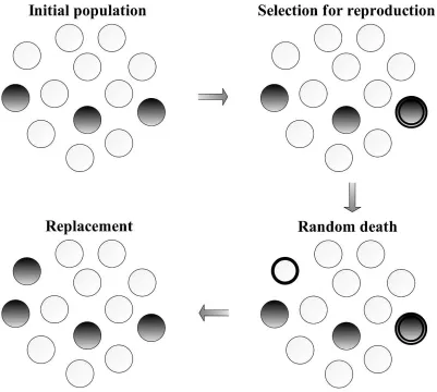
Figure 1.1: The Moran process with frequency dependent fitness. A finite population

con-sists of two types of individuals, A and B. In each time step, an individual is randomly selected for reproduction with probability proportional to its fitness. An individual is cho-sen for death at random. An identical offspring of the individual chocho-sen for reproduction replaces the dead individual. Hence, in each time step the population size remains constant.

So, there are some reasonable questions: What is the probability that a particular

type will fixate? How long will it take to fixate given that this will happen? How long will it take for one of the two types to fixate?

Consider a population consisting of two types of individuals, X and Y. The

fixa-tion probability of type X is the probability that at the end of the evolufixa-tionary process

the population will consist only of X individuals, i.e. the probability that X

individ-uals will spread over the whole population and fixate. The mean absorption time (or

unconditional fixation time) is the mean number of time steps needed to reach one

of the two absorbing states of the dynamics, i.e. the required time for the process to

end up either in the state where all individuals are of type X or in the state where all

individuals are of type Y. The mean fixation time (or conditional fixation time) of X

individuals is the number of time steps required for X individuals to take over the

(34)

Introduction

entire population, given that this will happen. Another quantity of potential interest

that we introduce in this work is the mean number of transitions to absorption or

fixation, where the number of transitions is defined as in the time, except that events

where the population size of one type of individuals (and thus that of the other) is

unchanged are not counted.

Expressions for the fixation probability as well as the mean fixation time were

derived in Karlin and Taylor (1975). The fixation probability has later been consid-ered in populations of finite size (Nowak et al., 2004; Taylor et al., 2004). Complete

derivations of the formulae of the fixation probability and the mean time to

absorp-tion and fixaabsorp-tion in a homogeneous populaabsorp-tion of finite size can be found in Antal

and Scheuring (2006) and Traulsen and Hauert (2009). In Appendix A we

repro-duce these derivations and in some cases we present alternative formulae. Note that

these formulae can be applied to stochastic evolutionary processes where there is

no mutation and in each time step the number of individuals of one type increases

by one, decreases by one or remains the same, and thus the population size remains

constant.

Consider a population of size N with two types of individuals, A and B. Ac-cording to the Moran process, the number of A individuals in each time step can

increase by one, decrease by one or remain the same, with some probabilities that

depend only on the current state of the system. Hence, the process is a Markov

pro-cess, which is essentially a discrete random walk on states 0≤i≤N with absorbing

boundaries. The transition matrix of the process is a tri-diagonal matrix with entries

pi,i+1=

i fA

i fA+ (N−i)fB

· N−i

N−1, 1≤i≤N−1, (1.24)

pi,i−1=

(N−i)fB

i fA+ (N−i)fB

· i

N−1, 1≤i≤N−1, (1.25)

pi,i=1−pi,i+1−pi,i−1, 1≤i≤N−1, (1.26) and zero everywhere else. Here, pi,j is the element in the ith row and jth column of

the transition matrix and denotes the transition probability from the state with i A

individuals to the state with j A individuals. At the absorbing states, p0,0=pN,N=1.

The fixation probability of i∈[1,N]A individuals in a finite well-mixed popula-tion of B individuals,APi, is given by (see Appendix A.1)

A_P i=

1+i−∑1

j=1

j

∏

k=1

qk

1+N∑−1

j=1

j

∏

k=1

qk

(35)

Introduction

where qk is the ratio of the probability of the number of A individuals being

de-creased by one, pk,k−1, and the probability of the number of A individuals being increased by one, pk,k+1, i.e. qk= pk,k−1/pk,k+1. Clearly, the probability of i A in-dividuals dying out, i.e. the fixation probability of N−i B individuals,BPi, is given

byBPi=1−APiwhich leads to B_P

i= N−1

∑

j=i j

∏

k=1

qk

1+N∑−1

j=1

j

∏

k=1

qk

. (1.28)

The (average) fixation probability of a single individual playing strategy X,XP1, will be denoted byXP.

In the case where each of A individuals has relative constant fitness equal to r,

when compared to the fitness of a B individual, the transition probabilities are

pi,i+1=

ir ir+N−i·

N−i

N−1, 1≤i≤N−1, (1.29)

pi,i−1=

N−i ir+N−i·

i

N−1, 1≤i≤N−1, (1.30)

pi,i=1−pi,i+1−pi,i−1, 1≤i≤N−1, (1.31)

p0,0=pN,N=1, (1.32)

and equal to zero in any other case. In this case q_k=1/r, and thus from the formula

(1.27) we obtain that in the Moran process the fixation probability of i∈[0,N] A individuals which have a constant fitness r times higher than that of B individuals,

A_P

Mi, is given by the simple formula

A_P

Mi=

1−r−i

1−r−N, r6=1 (1.33)

(the fixation probability of a single mutant A in the Moran process will be denoted

by APM). Hence, in contrast to the deterministic replicator dynamics (see Section 1.2), although individuals with fitness r>1 are favoured by selection (their fixation

probability is higher than that of a neutral individual, 1/N) their fixation is not

cer-tain, even in an infinitely large population. Similarly, although selection opposes the

fixation of individuals with fitness r<1 (their fixation probability is less than 1/N)

and thus their extinction is more likely, this is not certain. This occurs due to the fact that even the fittest individual might not be chosen for reproduction and even the

least fit individual might be chosen for reproduction. This random effect is called

(36)

Introduction

random drift and is very important in the evolution of finite populations, especially

when the population size is small. For r=1, we have the case of so-called neutral

drift, where all individuals have the same fitness. In this case, although there is no

natural selection, the frequencies A and B individuals will drift until one strategy

takes over the entire population. The fixation probability of i As in this case is equal

to i/N. This should be expected, since every individual can reproduce or die with

equal probability. Thus, every single individual has probability 1/N to take over the

entire population and fixate no matter its type; since there are i individuals of type

A, their probability to fixate is i/N.

The mean time to absorption when i∈[1,N] A individuals are introduced in a population of B individuals, Ti, is given by (see Appendix A.2)

Ti=APi N−1

∑

j=1

1

pj,j+1

N−1

∑

l=j

l

∏

k=j+1

qk− i−1

∑

j=1

1

pj,j+1

i−1

∑

l=j

l

∏

k=j+1

qk. (1.34)

The (average) time to absorption starting from a single individual playing strategy

X will be denoted byXT .

The fixation time of i∈[1,N]A individuals in a population of Bs,AFi, is given

by (see Appendix A.3)

A_F i=

N−1

∑

j=1

A_P j

pj,j+1

N−1

∑

l=j

l

∏

k=j+1

pk,k−1

pk,k+1

−_A1

Pi i−1

∑

j=1

A_P j

pj,j+1

i−1

∑

l=j

l

∏

k=j+1

pk,k−1

pk,k+1

. (1.35)

The (average) fixation time of a single individual playing strategy X,XF1, will be denoted by XF. The derivation of the mean time to fixation of B individuals can

be found in Antal and Scheuring (2006) and Traulsen and Hauert (2009). However,

these can also be derived from the formula (1.35) by symmetry arguments.

The above formulae are effectively a re-organisation of the ones in Traulsen and

Hauert (2009).

Note that in the Moran process, the mean fixation time of a single A individual

when it is introduced into a population of Bs,AF, is the same as the mean fixation

time of a single B when it is introduced into a population of As, BF, for every

intensity of selection and for all games. Thus, AF =B_{F irrespective of which of}

the two types of individuals has the highest chance to fixate into a population of the other type. This does not hold in the cases where more than one individual of one

type invades in a population of individuals of the other type (Taylor et al., 2006).

In order to find the mean number of transitions before absorption occurs, as well

as the mean number of transitions before the fixation of A individuals, we consider

(37)

Introduction

different state, i.e. in each time step the number of A individuals either increases

or decreases by one. The transition matrix of this process is a square matrix where

only the entries below and the entries above the main diagonal can be non-zero. The

elements of the transition matrix are

πi,i+1=

fA

fA+fB

, 1≤i≤N−1, (1.36)

πi,i−1=

fB

fA+fB

, 1≤i≤N−1, (1.37) and zero everywhere else.

The mean number of transitions before absorption and fixation of A

individu-als occurs, starting from i∈[1,N] As, is given by the formulae (1.34) and (1.35), respectively, where pi,i+1=πi,i+1and pi,i−1=πi,i−1.

1.5 The effect of spatial structure on the outcome of

the evolutionary process

As we have seen in the previous sections, the traditional theory of evolutionary game

dynamics is based on the assumption that populations are infinitely large and

well-mixed. However, real populations, ranging from biology and ecology to computer

science and socio-economics, are of finite size and exhibit some non-homogeneous

structure where any two individuals have not the same probability to meet. For

example, individuals might have a higher probability to interact with neighbouring

individuals than with distant individuals.

At its simplest, the spatial effects on the evolutionary game dynamics have been

considered by assuming that the individuals of the population are distributed over a spatial array and interact with their nearest neighbours (see for example, Nowak and

May, 1992, 1993; Nowak, 2006; Killingback and Doebeli, 1996; Szab´o and T˝oke,

1998; Hauert, 2002; Hauert and Doebeli, 2004; Szab´o and F´ath, 2007). This might

be a one-dimensional array, a two-dimensional array (e.g., triangular lattice, square

lattice, hexagonal lattice) or higher dimensional array (e.g., cubic). However,

biolog-ically only lattices of dimension one, two and three are of interest. Each individual

adopts a strategy from a finite number of strategies available to use. Individuals

up-date their strategy following either deterministic or stochastic upup-date rules. In the

deterministic evolutionary dynamics (in discrete time), in every generation each in-dividual updates its strategy and adopts the strategy which has obtained the highest

total payoff among its strategy and its neighbours’ strategies. The total payoff of

(38)

Introduction

Figure 1.2: A spatial evolutionary game. Here, individuals of the population occupy the

cells of a square lattice and each of them interacts with its 8 neighbours. The game played among the individuals is described by the payoff matrix (1.2). The payoff of each individ-ual at the end of each round is the sum of the payoffs obtained by the games played with each of its neighbours in the round. Every individual compares its payoff with that of its neighbours and adopts the strategy which resulted in the highest payoff. The figure shows the neighbourhood of an individual playing strategy A (black cells) when it is introduced in a population of individuals playing strategy B (white cells), from the end of the first round to the end of the second round in the case where b>d and 8b>c+7d.

each individual is the sum of the payoffs resulting from the interactions with each of the connected neighbours. The update of individuals’ strategy is synchronous, i.e.

all individuals update their strategy simultaneously in discrete time steps (see Figure

1.2). In stochastic evolutionary dynamics the update of strategies is asynchronous.

Randomly selected individuals update their strategy sequentially following some

stochastic update rules (but in each generation the number of such updates is equal

to the number of individuals occupying the sites of the lattice so that on average

every individual updates its strategy once). For example, an individual is chosen at

random and updates its strategy adopting the strategy of a random neighbour with a

higher payoff with a probability proportional to the difference of their payoffs. Nu-merous investigations of evolutionary games on different lattices and under different

dynamical processes have shown that the results of the evolutionary process might

be quantitatively and qualitatively different from the results obtained in the classical

evolutionary game theory. For example, although the classical evolutionary game

theory predicts that cooperators can never invade defectors in a Prisoner’s Dilemma

type of game, in the deterministic spatial Prisoner’s Dilemma, under some

condi-tions the survival of cooperators is possible and the two strategies can coexist in a

dynamic equilibrium (e.g., Nowak and May, 1992; Nowak, 2006). If the

Evolutionary models in structured populations

City, University of London Institutional Repository

Citation

:

This is the unspecified version of the paper.

This version of the publication may differ from the final published

version.

Permanent repository link: http://openaccess.city.ac.uk/1731/

Link to published version

:

Copyright and reuse:

City Research Online aims to make research

outputs of City, University of London available to a wider audience.

Copyright and Moral Rights remain with the author(s) and/or copyright

holders. URLs from City Research Online may be freely distributed and

linked to.

EVOLUTIONARY MODELS

IN

STRUCTURED POPULATIONS

Christoforos C. Hadjichrysanthou

Thesis submitted to City University London

for the degree of Doctor of Philosophy

City University London

School of Engineering and Mathematical Sciences

Centre for Mathematical Science

Contents

List of Figures

List of Tables

Acknowledgments

Declaration

CHAPTER 1

Introduction

1.1

Classical game theory

1.1.1

Dominant strategies and Nash equilibria

1.2

Evolutionary game theory

1.2.1

Evolutionarily Stable Strategies

1.2.2

Replicator Dynamics

1.3

Some classical games

1.3.1

The Hawk–Dove game

1.3.2

The Prisoner’s Dilemma game

1.3.3

Coordination games

1.3.4

The Snowdrift game

1.4

Stochastic evolutionary dynamics in finite

homo-geneous populations – The Moran process

∑

∑

∏

∑

∑

∏

∑

∑

∏

∑

∑

∏

1.5

The effect of spatial structure on the outcome of

the evolutionary process