Tuningless load frequency control through active engagement of distributed resources

Tuningless Load Frequency Control Through Active

Engagement of Distributed Resources

Alexander M. Prostejovsky,

Student Member, IEEE,

Mattia Marinelli,

Senior Member, IEEE,

Michel Rezkalla,

Student Member, IEEE,

Mazheruddin H. Syed,

Student Member, IEEE,

and Efren Guillo-Sansano,

Student Member, IEEE

Abstract—The increasing share of volatile and inverter-based energy sources render electric power grids increasingly suscepti-ble to disturbances. Established Load Frequency Controls (LFCs) schemes are rigid and require careful tuning, making them unsuitable for dynamically changing environments. In this paper, we present a fast and tuningless frequency control approach that tackles these shortcomings by means of modern grid monitoring and communications infrastructures in a two-fold concurrent process. First, direct observation of supply and demand enables fast power balancing decoupled from the total system dynamics. Second, primary resources are actively involved in frequency restoration by systematic adjustment of their frequency reference setpoints. In contrast to the commonly used Automatic Gen-eration Control (AGC), the proposed Direct Load Frequency Control (DLFC) does not require an integrator for frequency control in the closed loop even under partial grid observability. The approach is Lyapunov-stable for a wide range of system parameters, including ramping limits of controlled resources. A performance study against AGC has been conducted on a three-area power system in simulations as well as in a real laboratory grid with an installed generation capacity of110 kW.

Index Terms—Automatic Generation Control, Distributed Sys-tems, Load Frequency Control, Low Inertia SysSys-tems, Power Quality, Renewable Energy Sources, Web-of-Cells

I. INTRODUCTION

The increasing number of inverter-based Distributed Energy Resources (DERs) and High Voltage Direct Current (HVDC) tielines reduces the inertia of the power system and thereby its ability to withstand disturbances [1], [2]. Established Load Frequency Control (LFC) schemes, notably Automatic Gener-ation Control (AGC), have difficulties coping with the entailed changing dynamics and the volatility of renewable energy sources because of their rigid tuning requirements [3], [4]. A direct consequence is the rising number of frequency vio-lations as reported by the European Network of Transmission System Operators for Electricity (ENTSO-E) [5]. However, the blurring line between Transmission System Operators (TSOs) and Distribution System Operators (DSOs), the expanding monitoring infrastructure, and the availability of new flexibility resources opens new possibilities for LFC [6], [7], [8].

The work presented in this paper was supported by the European Commis-sion under the FP7 project ELECTRA (grant no: 609687).

A. M. Prostejovsky, M. Marinelli, and M. Rezkalla are with the Center for Electric Power and Energy, Technical University of Denmark, 4000 Roskilde, Denmark (e-mail: [email protected]).

M. H. Syed and E. Guillo-Sansano are with the Institute for Energy and Environment, Electronics and Electrical Engineering Department, University of Strathclyde, Glasgow, G1 1RD, Scotland.

The shift towards horizontally integrated grids entails an active management role for DSOs [9]. Their biggest asset is awareness of the available flexibility through monitoring the infrastructure close to the customers and DERs [10]. The ongoing roll-out of Smart Meters (SMs) and Remote Terminal Units (RTUs) [11] steadily increases the monitoring coverage of distribution grids, whose economical and technical benefits for real-time control are highlighted by the European Commission [12], [13]. Information and Communication Tech-nology (ICT) is the key enabling factor, for which reason the development of data management policies, standardized data exchange, and TSO-DSO data interfaces, is being actively pursued [14]. Currently, these efforts are focused on the energy retail market, but regulatory authorities and System Operators (SOs) emphasize the benefits of harnessing flexibility at the distribution level. Regulatory issues concerning data ownership and privacy, as well as questions about the hierarchies between TSOs, DSOs, and third parties, such as aggregators, remain open so far. Nevertheless, it is reasonable to assume that a near-complete observability of the electric grid will be achieved in the foreseeable future.

This paper presents a fast and tuningless LFC approach called Direct Load Frequency Control (DLFC), suitable for dynamically changing power grids, which harnesses modern means of monitoring and communication under the assumption of reasonably high grid observability. The DLFC is simple, consisting only of two algebraic equations and first-order low-pass filters describing two concurrent processes. First, area imbalances are obtained through direct observation of production and consumption, which enables the fast activation of secondary resources. Second, primary resources are actively involved in frequency restoration by systematically adjusting their frequency references. The frequency is effectively treated as a local quantity in our method, as we infer it over the primary resources’ output state with regard to their nominal setpoints. The resulting control loop is largely decoupled from the non-linearities of the actuators; secondary power is only activated in response to local events; and no integrators are required to mitigate steady-state errors if the primary droop capabilities are well-known. Active state data exchange between neighboring areas enables load sharing, and the only free parameter is the control interval.

via an auxiliary term. The auxiliary hook can furthermore be used for other corrective terms like tertiary control, or time synchronization. Analytical and experimental examinations prove the DLFC’s ability to regulate the frequency for a wide range of disturbances, parameters, and uncertainties, as well as under conditions of partial observability and controllability. Its performance stands up to optimally tuned AGCs without the associated parametrization effort.

This paper is structured as follows. Section II-A features a literature review of related works, a detailed description of AGC, and an overview of the proposed DLFC approach. Section III contains the grid model and derivation of the DLFC along with a stability proof using Lyapunov’s direct method. Section IV covers the experimental setup, corresponding parameters, and implementation considerations for verifying the DLFC’s applicability. Section V contains performance comparisons of AGC and DLFC under changing physical parameters using simulations, as well as the experimental verification in the laboratory grid along with a discussion of the results. Finally, Section VI concludes the findings and addresses open issues and potential future research.

II. COMPARATIVESTUDY

This section presents an overview of the literature related to the proposed approach. With AGC being commonly used in present-day secondary control, it is introduced in detail and used as the reference implementation. Its description also sets the scene for the grid modeling in Section III.

A. Literature Review

Studies on LFC for interconnected power systems predomi-nantly focus on two categories: adaptive approaches and Multi-objective Optimization Problems (MOPs).

The PI controllers used by AGC require tuning to achieve the desired performance while ensuring stable operation. Adaptive tuning aims to automatize this process with mini-mal model knowledge. The adaptive controller used in [15] observes the Area Control Error (ACE) of all involved control areas to calculate a global gain correction factor. Mathematical optimization is performed in [4] using an event-triggered, adaptive dynamic programming approach, whereas [16] relies on sequential quadratic programming taking into consideration the governor limits. The approach in [17] uses a special observer for the chaotic behavior of interconnected controllers as an input to the optimization problem. Machine learning is another take on adaptive control, which operates by observing solely performance metrics without models. Examples are the fuzzy control approach in [18] and the Adaptive Neuro-Fuzzy Inference System (ANFIS) approach in [19].

MOPs aim to find optimal setpoints based on the observed states and underlying physical models. Model Predictive Con-trol (MPC) incorporates the current and future constraints on a system to solve the MOP. A centralized approach suitable for smaller synchronous areas, like the Nordic grid, is inves-tigated in [20]. The distributed MPC (DMPC) presented in [21] decomposes large problems into smaller ones, which are then solved independently and reassembled using active data

exchange. Parameter uncertainties are explicitly accounted for by the robust DMPC approach in [22].

In-depth reviews of the mentioned control strategies and many more are presented in [23], [24]. Compared to the proposed DLFC, however, most approaches have drawbacks regarding their practical realization. The stability of adaptive controllers in interconnected systems is difficult to prove, particularly in the presence of the time delays inherent in ICT-based systems [25]. On the other hand, approaches requiring accurate state-space representations are strongly dependent on the accuracy of the model. The complexity of large-scale grids in the presence of the rising number of DERs, faster system dynamics, as well as the necessity of deploying distributed versions of the algorithms across utilities, render the implementation of approaches like MOP very challenging.

B. Automatic Generation Control

AGC is widely used in secondary control for its simplicity and well-understood behavior. Its input signal is the ACE P_iACE = ∆P_itie +Bi∆fi, with the tieline error ∆Pitie =

Ptie

i − P

tie

i,0 and the bias factor Bi [26]. The net power

interchange Ptie _{between neighboring areas is scheduled at} Ptie

0 . The bias factor is an estimation of the area’s droop gain

(frequency-response characteristic) ki = _R1

i +Di, including

the primary devices’ speed droopRi and the damping factor

Di of frequency dependent loads. AGCs are typically realized

as PI-controllers

Pisec =ViPPiACE+ 1

TI i

∫ t

t0

PiACE(τ)dτ (1)

using the proportional gain VP

i and the integral time

con-stant TI

i. The determination of these parameters is done by

observing the area response to major grid events (such as a tripping prime mover), with further adjustments during normal operation. The resulting secondary power setpoint Psec

i gets

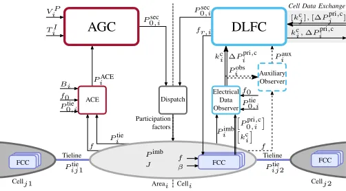
subsequently dispatched to the units participating in secondary control. Fig. 1 shows the corresponding signal flows.

C. Overview of the Proposed Approach

The DLFC is based on a set of assumptions regarding ICT and monitoring as described in Section I, which transcends the capabilities of traditional control areas. Therefore, we refer to them as Cells to provide a clear distinction. More information on the Web-of-Cells concept can be found in [27] and [28].

AGC

ACE

P_itie

f

f0

Bi P

ACE

i

V P_i

P₀sec_,i

P₀tie_,i

Auxiliary Observer

P_iaux

[k_jc],[∆P_jpri,c]

f

k_ic,∆P_ipri,c

Cell Data Exchange

Celli

Tieline Tieline

Cellj1 Cellj2

FCC FCC

T I_i

Dispatch

P₀sec_,i

DLFC

fr,i

FCC

Pimb

J f_β

P_ijtie₁ P_ijtie₂

Participation factors

Electrical Data Observer

∆P_ipri,c

kc_i

P_iobs

f0

P₀tie_,i

Areai

[

P₀pri_,i,c]

[

kc_i]

P_iimb

Fig. 1. Structural overview of AGC versus DLFC signal flows.

The signal flows of the DLFC and the AGC are shown side-by-side in Fig. 1. On the DLFC side, the EDO acquires state information from the Cell, and the auxiliary block allows for incorporating additional corrective powers. The primary devices perform Frequency Containment Control (FCC) and actively participate in secondary control as part of the method. The FCCs report their droop gains and output powers to the EDO, which forwards the aggregate values to the DLFC, and takes the reference frequency signal in return. Neighboring Cells appear as atomic devices with droop capabilities, and as such they exchange state information, similarly to the FCCs. Both LFCs feed their power regulation signal into a dispatcher that evaluates the participation factors for all plants bidding into secondary control. Economic dispatch strategies for liberalized grids can be found in [30]. The mathematical description of the DLFC is presented in the following section.

III. METHODOLOGY

The DLFC formulation uses the definitions of variables in Section II-B and Fig. 1, a generation-oriented frame of refer-ence (power flows into Cells are positive), and the constants are positive where applicable.

A. Cell Modeling

The change of frequency (rotational speed of synchronous generators) is a function of generation and load imbalances Pimb _{described by the swing equation}

J ωω˙ =Pimb (2) with the inertia J and the (angular) frequency ω = 2πf [26]. Within a synchronous areaA, we define a neighborhood

N Hi={i,ACi} ⊆ A to describe its dynamic behavior using

(2). The Cell under consideration is denoted byi, andj∈ ACi are the adjacent Cells coupled over tie-lines with the breaker state δij(n). The neighborhood is described by

J =Jpri,c_+Juc_=J

i+

∑

j_∈ACi

δijJj, (3)

Pimb=Ppri,c+Ppri,uc+Pc+Puc+Ptie+Puo

=P_iimb+ ∑

j∈ACi

δijPjimb. (4)

Jpri,c _{is the combined inertia of the controllable synchronous} machines, whereasJuc_{includes uncontrollable generators and} other resources like synchronous condensers.Ppri,c_andPpri,uc are the active power contributions of the controllable and uncontrollable primary resources (including synchronous ma-chines, inverter-based devices and frequency-dependent loads), Pc _{is that of the directly controllable devices and} aggre-gated flexibility resources, Puc _{is that of the uncontrollable} resources, and Ptie _{is the net interchange over tielines. P}uo represents the unobserved generation and consumption that lacks direct feedback into the control loop. The power output of the primary resources is

Ppri=P₀pri−k∆f, (5) with the resources’ power being P₀pri atf0, their total droop

gaink, and the frequency deviation ∆f =f−fr. The

refer-ence frequencyfrcan be remotely adjusted on the controllable

primary resources and isf0 for all others.

B. Proposed Secondary Control

The DLFC consists of two concurrently operating control stages that enable frequency control without the need for an integrator. Direct observations of electric power production and consumption are used to to determine the secondary power setpoint, and remaining mismatches (e.g., due to par-tial observability or measurement errors) are systematically captured by primary resources. The tasks of primary (droop control) and secondary (balancing) resources of established control schemes are preserved but their activation is conducted differently, which is described in the following.

Secondary control executes at intervals ofTcsec; the integer nindexes the discrete-time sequencet=nTsec

c .

1) Direct Power Balancing: The ACE infers the area im-balance over the measured frequency and the tielines’ active power flows. Both quantities are dynamically coupled to the primary response of the whole synchronous area, against which the AGC’ PI-parameters need to be tuned. The DLFC circumvents this issue by using the aggregate power balances from within the area instead of the area boundaries. Deter-mination of secondary power setpoints is therefore decoupled from the external grid.

The total observable power of one Cell is

Pobs

i (n) =P

pri,uc

i (n) +P

uc

i (n) +P

pri,c

0,i (n) +P

tie

i,0(n), (6)

with the sum of all closed tieline schedules,

P₀tie_,i(n) = ∑

j_∈ACi

δijP0tie,ij(n), (7)

features all powers of (3) directly captured by the metering system. One notable difference is the use of setpoint values instead of actual measured states for some quantities. State information about primary resources’ deviations from their intended setpoints are needed for frequency control in Sec-tion III-B2, whereas the avoidance of the actual state of tielines decouples the power balancing response from the other Cells. The optimal secondary power setpoint therefore becomes

with the auxiliary power term Paux

i used for hooking in

additional corrective terms (e.g., tieline observers to detect re-maining load or generation unobserved by the power matching stage, or time corrections). Mismatches of observed and actual imbalances are handled in the next step.

2) Primary Frequency Control: Primary resources adjust their power output based on the locally measured frequency, as described in (5). The frequency can therefore be found indirectly, by means of the deviation of the resources’ output from their operating points at f0, according to ∆Ppri,c =

Ppri,c_−Ppri,c

0 = −kc∆f. This effectively expresses the

fre-quency as a local instead of a global quantity, which the DLFC then uses for systematically adjusting the primary reference frequencyfrwithin the Cell. Hence, a Cell’s secondary control

reacts as quickly as allowed by its primary and secondary resources together, irrespectively of the dynamics of the rest of the synchronous system.

The steady-state balance neighborhood N Hi is

0 = ∆Ppri,c+ ∆Ppri,uc+ ∆Ptie+Puo, (9) with the primary resources covering∆Ptie_+Puo_{, which is not} compensated by the power balancing stage in Section III-B1. Applying ∆Ppri,c =−kc(f−fr)to (9) and rearranging for

fr results in fr = f − _k1c(∆P

pri,uc_{+ ∆P}tie _+Puo_{), which} is equivalent to fr =f + ∆P

pri,c

kc . Setting f = f0 yields the

optimal reference frequency

f_r,i∗ (n+ 1) =f0+

∆P_ipri,c(n)+∑_j∈AC

iδj(n)∆P

pri,c

j (n)

ˇ

kc

i(n)+

∑

j∈ACiδj(n)ˇk

c

j(n)

(10)

for any given steady-state deviation ∆Ppri,c _{inN Hi. As (9)} also includes the tieline states, the collectivity of Cells are able to cover for saturated Cells that are unable to provide balancing capability.

Assuming that the effective droop gain kc _{is not precisely} known, the adjusted value ˇkc_{= ˆk}c_{(1 +ϵ)is used in (10) to} prove stability in Section III-C. Here, the best estimate ofkc is kˆc_{, which gets slightly increased by the relaxation termϵ.} Choosing ϵ= 2σ, σ being the variance ofˆkc, yields a95 %

probability that ˇkc≥kc.

3) Low-pass Filtering: Low-pass filtering of the optimal balancing powerP_isec,∗(n+1)and reference frequencyf_r,i∗ (n+ 1)serves several purposes in the DLFC: it suppresses measure-ment noise as well as aliasing effects from the discrete-time sampling, it smooths the secondary response, and it increases the stability margin. The filtered signals

P_isec(n+ 1) =P_isec(n) +TcωLP

2π (

P_isec,∗(n+ 1)−P_isec(n)), (11) fr,i(n+ 1) =fr,i(n) +Tc₂ω_πLP

(

f_r,i∗ (n+ 1)−fr,i(n) )

, (12)

are acquired using the filter cutoff ωLP and are sent to the secondary dispatcher and the primary devices, respectively. The filter cutoff is the only free parameter in the controller and must respect the control interval’s Nyquist frequency

ωLP<Tπc. (13) It can otherwise be chosen as fast as the quality of the input signals allows, which renders the DLFC tuningless.

C. Proof of Stability

The stability of the closed control loop is assessed on the continuous system using Lyapunov’s second method [26]. A Lyapunov candidateV(x) :Rm_{→Ris any function that}

ful-fills the propertyV(0) = 0for the equilibriumxSS=0. The system is stable if ∀x:V(x)≥0and∀x\ {0}: ˙V(x)≤0, andV(x) is then called the Lyapunov function.

1) Continuous System Representation: We transform the discrete-time controllers using the forward Euler method y(n+ 1) =y(n) +Tsec

c f(y(n))and rearrangef(y(n))to the left side to obtain a continuous representation of the system1_. Using Eqs. (2)–(8) and (10)–(12) we obtain

˙

z=fz(z) =     

−kc_(f−f

r)−kuc(f−f0)+Pe+Psec

J f

−ωLP

(

Pe_γobs_+Psec)

f0−fr−γc(f−fr)

Tc ωLP(fr∗−fr)

   

, (14)

with the state vector z = [f, Psec_{, f}∗

r, fr]⊤, the exogenous

inputPe_{, the ratioγ}obs_=|Pobs

Pe |representing how much ofP e is observed, and the droop gain distortion γc=k_kˆcc.

The proof requires f(0) = 0, hence a coordinate trans-formation of (14) is necessary. Solving fz(zSS) =0 for the steady-state solution zSS and introducing x = z −zSS =

[x1, x2, x3, x4]⊤ yields

˙

x=fx(x) =fz(x+zSS). (15)

2) Lyapunov Function: The chosen Lyapunov candidate is

V(x) =J x2₁(γ

ϵ_+γϵ_γuc_−γuc₎(2

3x1+f0

)

kc_+Pe_(1−γobs_)(1−γϵ₎

2(kc₎2_((γuc_+1)γϵ_−γuc₎

+J f0

x2₂+kc(βx2₃γϵ+x2₄)

2αβ(kc)2_(γuc+1) .

(16)

with the droop gain overestimation factorγϵ =γc_{(1 +ϵ)≥}

1, the ratio of uncontrolled to controlled primary resources γuc= k_kucc ≥0, as well as the placeholders α=

J f0

Tck >0 and

β=Tcfc∈(0,1).

The total time derivative of (16) is

˙

V(x) =−(1 +γuc_)x2 1−x

2 2−γ

ϵ_x2 3−x

2 4

+x1(x2−x3+x4) + 2x3x4.

(17)

Forγuc_{≥0 andγ}ϵ_{≥1, (17) fulfills} ˙

V(x)≤ −x22+(x1+x3−x4)2+(x1−x2)2+(x4−x3)2

2 ≤0. (18)

3) Stability Assessment: An investigation of (16) reveals that either for perfect knowledge of the droop gain of control-lable resources (γϵ_{= 1) or total observability (γ}obs_{= 1), the} Lyapunov function is decoupled from the power disturbance Pe _{and stable for ∀x}

1 ≥ −3₂f0, which is always fulfilled.

Otherwise, the minimal stability range for arbitrary power disturbances is

Pe(_1−γobs)_(1−γϵ_{)≤ |k}c_(γϵ_−γuc_(1−γϵ_))f

0| (19)

1_{Applying the bilinear transform would require the incorporation of fast}

NEV IC 1 NEV IC 2 NEV IC 3 NEV IC 4 NEV IC 5 NEV IC 6 NEV IC 7 NEV IC 8 Lab busbar Grid busbar Busbar 1 Busbar 2 630 kVA 100 kVA Battery Ext. 117-5 Cabl e C2 Cabl e C1 Mobi le Load 1 Ext. 117-2

Chg. post Cabl

e D1 Sola r NEV IC Busbar A Busbar B Busbar C 150 kVA 100 kVA Gaia Flexhouse Solar Cable B1 Cable B2

Busbar 1 Busbar 2

Local busbar 200 kVA Dumpload Diesel EV Aircon Cable A1 Cable A2 Solar Grid busbar Busbar 1 Busbar 2

Cable F1 Cable E1 Cable E2 Mobile Load 3 CHP Heatpump 1 Heatpump 2 Cable F1 Crossbar switch Load Conv. SYSLAB breaker overview

Switchboard 716-2 Switchboard 715-2 Switchboard 319-2

NEVIC Ship Shore Mach. set Test bench 1 Test bench 2 Test bench 3 Switchboard 117-2 Flexhouse 2 Flexhouse 3 Tieline 3-1 Tieline 1-2 Tieline 2-3 Cell 1 Cell 2 Cell 3 Tieline 3-1 Tieline 1-2 Tieline 2-3 715-2.1 716-2.1 319-3.A 319-2.Local 350m 25m ~ Gaia = ~ Solar Dump load = ~ Battery E1 A1 319-3.C 117-2.1 = ~ Solar 250mB2 = ~ Solar ~ Aircon Diesel Flex house 1

650mC2 650mC1 25mA2 Cell 3 Cell 2 Cell 1 EV Mobile load 3 Mobile load 1

Primary Secondary Inertia response Observable Unobservable

I/II

I, J II

II

I II J Breaker open/closed

syslab-09

syslab-01

syslab-11

Java RMI

ØMQ Subscribe ØMQ Subscribe

Java RMI Java RMI ØMQ Publ. ØMQ Publ. ØMQ Publ. Device Comm.

Cell level Comm.

Fig. 2. Laboratory layout (used configuration marked in red) and correspond-ing scorrespond-ingle line diagram together with the communication infrastructure.

for |x1| ≪ f0. Because the droop of typical power systems

ranges from 1 % to 10 %, kf0 is much larger than the total

installed power and|Pe_{|is therefore always within the stability} range during normal operation.

A closer examination of the proof reveals an advantageous property of the DLFC regarding nonlinearities: Ramp limi-tations of the primary devices participating in the secondary control result in temporarily decreased effective droop gains. Since we showed before that overestimation of the gains increases the stability margin, ramp limitations contribute to the stability of the DLFC, unlike the case of the AGC, where the integrator winds up.

IV. SYSTEMCHARACTERISTICS

The applicability of the proposed DLFC has been verified both in simulations and in a laboratory grid featuring industrial power and metering devices. In the following, the experimental setup and implementation aspects are described.

A. Experimental Setup

The experimental facility SYSLAB, located at the Risø cam-pus of the Technical University of Denmark, is a400 V three-phase grid designed for studying advanced grid control and communication concepts. It has 16 busbars and 116 automated coupling points, as shown in Fig. 2, spread across an area with a diameter of about 1 km. A wide range of DERs (wind turbines, solar panels, a Diesel generator, controllable loads)

TABLE I

PROPERTIES OF DEVICES USED IN THE EXPERIMENT

Device Cell Busbar Pnom Pmin Pmax P0 Ctrl. Obs. Description

(kW) (kW) (kW) (kW)

Aircon 1 319-2.L 9.8 0.0 9.8 - ✓Wind turbine

Battery 2 117-2.1 0.0 −15.0 15.0 −5.0 I/II ✓Vanadium redox flow type,190 kWh

Cable A1 3

1

319-3.A

319-2.L 4.0 ✓

Tieline 3-1,R= 8.02 mΩ,

X= 1.95 mΩ,25 m

Cable C1 1

2

319-3.C

117-2.1 −4.04 ✓

Tieline 1-2,R= 97.0 mΩ,

X= 55.9 mΩ,650 m

Cable C2 2

3

117-2.1

319-3.A 4.01 ✓

Tieline 2-3,R= 88.9 mΩ,

X= 54.0 mΩ,650 m

Dumpload 2 319-2.L−78.09−78.09 0.0 II ✓Resistor load bank, 256 steps EV 3 715-2.1 −2.0 −2.0 0.0 ✓Citro¨en C1, single phase charger Flexhouse 1 3 715-2.1 −25.0 −25.0 0.0 ✓Electric lights and heaters

Diesel 1 319-2.L 48.0 0.0 48.0 ₍10₁₁._.0₉₎ I ✓IVECO GE806Ii06, 2 pole pairs,_{S= 60 kVA,J= 2 kg m2}

Gaia 3 715-2.1 11.0 0.0 11.0 ✓Wind turbine

Mob. Load 1 2 117-2.1 −33.0 −33.0 0.0 ✓ Thyristor-contr., reactive power varieswith the firing angle between

0. . .16.5kVAr

Mob. Load 3 3 716-2.1 −33.0 −33.0 0.0 II ✓See Mobile Load 1 Solar 1 319-2.L 10.1 0.0 10.1 ✓Orientation az.180◦, el.40◦

Solar 2 117-2.1 10.1 0.0 10.1 ✓Orientation az.100◦, el.20◦

Solar 3 715-2.1 5.94 0.0 5.94 ✓Orientation az.190◦, el.60◦

Cells Totals −76.15−186.09 109.94 Sum over all devices

syslab-01 2Platform: Arch Linux, 64 bit, kernel 4-8-4-1-ARCH, Java 1.8.0 60; syslab-09 3Publish-subscribe communications between Cells using JeroMQ 0.3.6; syslab-11 1Push-pull communications between Cells and devices using JavaRMI.

can be remotely operated in various topological configurations over a distributed monitoring and control platform.

The system configuration used in Fig. 2 is made up of three Cells in meshed topology. Connected parts are marked in red and emphasized in the corresponding single-line diagram underneath, followed by the location of the Cell controllers as well as the communication links between them and the devices. The properties of the components are listed in Table I, where Pnom is the nominal device power, Pmin and Pmax are the lower and upper limits of the operating range, and P0 is

the base operating point, where applicable. Devices providing the primary response are marked with I, and II indicates participation in the secondary control. The diesel operates at a fixed droop of5 %as the grid-forming unit in island mode, and is the only component with a rotating mass. It covers, together with the four-quadrant inverter of the vanadium redox battery, the reactive power flows caused by cables and thyristors.

B. DLFC Implementation

a) Controller Settings: The secondary control is executed at intervals ofTsec

c = 1 sin all scenarios. The low-pass cutoff frequency isωLP= 1₃ according to (13).

b) Frequency Control: Remote adjustment of the ref-erence frequency fr on selected primary resources during

operation is required by the DLFC. The diesel supports this feature via its off-the-shelf governor, as does the battery via a custom-built controller.

TABLE II

CELL PROPERTIES FOR THE CONSIDERED SIMULATION SCENARIOS

Scenario Jhi Jlo

Cell 1 2 3 1 2 3

Inertia constantH(s)@S_base= 60 kVA 4.112 4.112 0.411 0.411 0.411 0.041

Ramp limitPramp(kW s−1 ) 2 5 10 20 50 10

Secondary delayT_delaysec (s) 5 2.5 1 0.5 0.25 0.1

Primary regulating capacity(kW) 48 30 0 48 30 0

Primary droop gainkc(kW Hz−1 ) 19.2 9.6 0.0 19.2 9.6 0.0

Primary droop(%) 5.00 6.25 0.0 5.00 6.25 0.0

AGC proportional gainV P(1) 0.065 0.09 0.1 0.065 0.09 0.1

AGC integral time constantT I(s) 12.5 9.091 7.691 12.5 9.091 7.691

Secondary control intervalT_csec(s) 1

DLFC low-pass filter cutoffωLP(rad s−1 ) 0.333(see Section IV-B)

TABLE III

SIMULATION EVENTS

Event Time(s) Parameter Parameter change Description

1 10 ∆P₁obs(kW) 0→ −5 Load in Cell 1 increased

2 50 ∆P₁obs(kW) −5→0 Load in Cell 1 decreased

3 90 ∆P₃obs(kW) 0→5 Load in Cell 3 decreased

4 130 ∆P₂uo(kW) 0→5 Load in Cell 2 decreased, unobs. by DLFC 5 170 ∆P₂uo(kW) 5→0 Load in Cell 2 increased, unobs. by DLFC

6 210

δ₁₂ 1→0

Tieline 1-2 opens, tieline setpoint sums for Cells adjust according to (7)

P₀tie_,1(kW)−8.08→ −4.04

P₀tie_,2(kW) 8→4

7 250 ∆P₃obs(kW) 5→0 Load in Cell 3 increased

V. RESULTS& DISCUSSION

A. Simulation

The simulation model of SYSLAB in Section IV-A was developed in MATLAB/Simulink. Each Cell is modeled us-ing one swus-ing equation (2) and the physical resources in Section III-A, incorporating the following constraints: Output saturations, ramping ratePramp limiting the change of primary and secondary power, and the reaction timeTsec

delayof secondary resources. Tielines are modeled as serial admittances as de-scribed in [31] without the parallel susceptances.

The DLFC is compared with the AGC for a range of Cell inertias, ramp rates, and control delays. Table II lists the parameters for two scenarios: (i) The high inertia scenario Jhi with long delay times and comparatively low ramp rates of primary and secondary resources, representing mechanical fuel-driven generators; and (ii) the low inertia scenario Jlo resembling SYSLAB setup with fast, inverter-based devices. Cell 3 offers in both scenarios only secondary power control, as it lacks primary resources. Despite Cells 2 and 3 having only inverter-coupled devices in the laboratory, a small inertia value is necessary for simulations.

The frequency deviation ∆f5% = 201|P

step_|(∑

Ak)−1,

which is5 %of the primary system response toP₀stepin steady-state, serves as a threshold to assess the settling time Tset for the controllers.Tsetis the interval between a load step and the point when|∆f|=|f−f0|remains smaller than∆f5%for all

times, formally Tset={Tset∈R| ∀t≥Tset:|∆f| ≤ ∆f5%}.

49.8 49.85 49.90 49.95 50.00 50.05 50.10 50.15 50.20

(a)

1 2 3 4 5 6 7

f

in

Hz

AGC,J_hi DLFC,J_hi AGC,J_lo DLFC,J_lo

0 25 50 75 100 125 150 175 200 225 250 275 300

49.90 49.95 50.00 50.05 50.10 50.15

(b)

Time ins

fr

in

Hz

Cell1, Jhi Cell2, Jhi Cell1, Jlo Cell2, Jlo

Fig. 3. Resulting frequencies for AGC and DLFC in (a) and DLFC reference frequencies in (b) for the two simulated scenarios. The grey lines illustrate the exponentially bounded response as defined by the ENTSO-E in [32].

We measure overshooting by the deviation of the relative frequency ∆frel = |

fmax−f0|

|fmin−f0|, where fmax is the maximum

andfmin is the minimum frequency after the load event. This ratio indicates by how much the system frequency rises above its nominal value in relation to the minimum detected value, which is predominantly determined by the primary response.

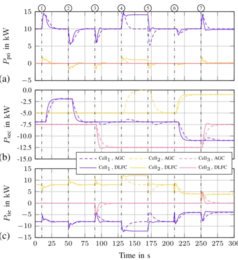
1) Event Response Evaluation: The series of events listed in Table III is applied in each scenario to the system for a simulation period of 300 s: Observed load steps; load steps unobserved by the DLFC; and breaking the meshed topology into a radial configuration by opening tieline 1-2. All load steps are ±5 kW, to which the parameters of the AGC’s PI-controller are tuned in theJhi scenario so as to deliver a fast and smooth response under the nonlinearities.

Fig. 3a shows the system frequency response for both scenarios and controllers. In scenario Jhi, the frequency ap-proaches 50±0.1 Hz after the initial inertia response due to the large secondary control delays. As the AGC was tuned for

±5 kW steps for optimal performance and no overshooting, its performance is similar for all events, with a settling time of around 20.02 s. The DLFC with a 26.08 s settling time is about 25 % slower in comparison, and exhibits around 40 %

overshooting due to the two concurrent control actions for the observed load events 1 to 4. Both controllers’ responses are bounded by exponentially decaying functions (“trumpet-curves”) defined byH(t) =f0±Ae−

t/T _{in [32]. For the case}

of the slowest DLFC responses (events 1 and 2), the trumpet parameters areA= 0.21 Hz andT = 14.5 s. This results in a decay time of 34 s to cross the ±20 mHzmargin around the nominal frequencyf0 after the event, which is well under the

900 srestoration time demanded by the ENTSO-E.

The primary reference frequencies fr, necessary for

−5 0 5 10 15

(a)

1 2 3 4 5 6 7

Ppri

in

kW

0 25 50 75 100 125 150 175 200 225 250 275 300 −15

−10 −5 0 5 10 15

(c)

Time in s

Ptie

in

kW

-15.0 -12.5 -10.0 -7.5 -5.0 -2.5 0.0

(b)

Psec

in

kW

Cell1,AGC Cell2,AGC Cell3,AGC Cell1,DLFC Cell2,DLFC Cell3,DLFC

Fig. 4. Resulting primary (a), secondary (b) and tieline (c) powers for AGC and DLFC for the two simulated scenarios. The legend applies to all subfigures.

responses immediately after the load events. As the secondary balancing resources start acting,frreturns tof0as the primary

powers approach their nominal operating points P₀pri. No overshooting occurs for unobserved events 5 and 6 because no direct power balancing takes place, and fr differs from

f0 as long as the unobserved power persists. The overall

reaction time is decreased in this case. Opening the tieline at event 7 makes Cell 3, which does not participate in primary control, the only physical neighbor of Cells 1 and 2. Hence, the reference frequencies start to diverge because of the different local ramp rates. Load sharing between the Cells is no longer proportional, but stable frequency control is maintained.

The situation between the controllers turns in the Jlo sce-nario where the DLFC only needs16.2 sto settle, approaching the 95 % settling time of 9 s for a first-order low-pass filter with a cutoff of ωLP = 3 rad s−1. Overshooting drops to around14 %. The AGC does not benefit from the faster system response and its performance gets even worse, causing even longer frequency excursions.

The powers in Fig. 4 reveal the fundamentally different behavior of AGC and DLFC. Fig. 4a shows the active in-volvement of the primary resources in frequency control, as opposed to the normal droop response with AGC. In the case of the secondary power response in Fig. 4b, AGC responds to all deviations in frequency or tieline during transients, causing secondary resource activations in Cells 1 and 2 (but not Cell 3, which lacks frequency dependent resources) regardless of the location of the event. The DLFC, on the other hand, only activates secondary resources if the event happened in its corresponding Cell, with the primary resources catching unobserved events. Consequently, the tieline power deviations

10 5 2 1 0.25 1.00 1.75 2.50

10 20 30 40 50

µspeed µstep

Tset

in

s

AGC

10 5 2 1 0.25 1.00 1.75 2.50

5 10 15 20 25

µspeed µstep

Tset

in

s

DLFC

10 20 30 40 50

Tsetins

Fig. 5. Settling time of AGC versus DLFC for variations of the disturbance step size and Cell response speed.

10 5 2 1 0.25_1.00

1.75_2.50

10−1 100

µspeed µstep

∆

frel

in

1

DLFC

0.100 0.158 0.251 0.398 0.631

∆frelin1

Fig. 6. Relative frequency overshoot of the DLFC for variations of the disturbance step size and Cell response speed.

caused by observed events and topological changes are miti-gated faster than by the AGC.

Events not directly captured by the system, however, cause deviations in the primary devices and tielines that need to be addressed with dedicated observers over the auxiliary hook in (6). It has to be noted that events 5 and 6 are merely meant to demonstrate the DLFC’s frequency control capability even when significant load changes are not captured by the measurement system. Under normal operation, entirely unob-served load events in the magnitude of the rated generation are highly unlikely to occur. Thus, tieline deviations would be considerably smaller in practice.

2) Sensitivity Analysis: That the DLFC is tuningless, unlike the AGC, is quantified by analyzing the system response to a single load step in Cell 1 for parameter variations between the two extremal cases of Table II. The multiplierµstep scales the step’s magnitude by Pstep _=µstepPstep

0 . In Cells 1 and 2

the multiplier µspeed scales the Cells’ inertias and ramp rates by J = µ−_speed1 J and Pramp =µspeedPramp,hi, respectively. The

changing environmental conditions. Smaller load steps and/or faster system responses lead to short settling times in virtually all considered cases, without the need for tuning.

The overshooting characteristic of the DLFC for variations of µstep and µspeed is depicted in Fig. 6. As demonstrated before in Fig. 3, the maximum peak recedes with faster system parameters. Variations of the step size reveal that the relative overshooting decreases with bigger steps. Thus, ramp limitations dampen the control response and increase the stability margins, as predicted by the stability proof in Section III-C. In contrast, the AGC requires careful tuning to prevent the controller’s integral term from winding up.

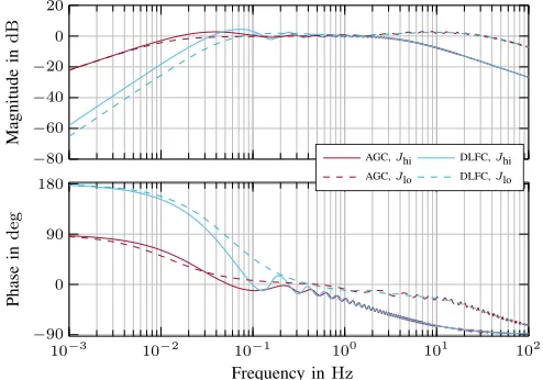
3) Small-Signal Analysis: A small-signal analysis has been conducted on the three-area system to study the frequency response of the two simulation scenarios described in Sec-tion V-A. The system is analytically linearized around f0 in

steady-state and includes secondary response delays, which are a degrading performance factor particularly in the high inertia case. System input is the load disturbance in Cell 1, and the output is the system frequency. The magnitude of the frequency response is normalized to the combined droop gain of the three Cells, for which the parameters of Table II apply. Fig. 7 shows the response for the AGC and DLFC in the high and low inertia cases. Both controllers behave similarly in the natural system frequency range between0.1 Hzto1 Hz

determined by the inertia constants and primary response. There, the response magnitude is mainly determined by the total droop capability of the three-area system. The AGC was optimally tuned for the high inertia case and consequently exhibits a smoother response than the DLFC in the considered range. Inertia dominates the suppression of higher frequency disturbances, resulting in a −20 dBfalloff in all investigated cases. The performance gain of the DLFC over the AGC is apparent for lower frequencies. Whereas the AGC shows a

−20 dBfalloff towards lower frequencies due to its integrator, the DLFC has−40 dBbecause of the concurrent power match-ing and reference frequency control mechanisms. Additionally, the DLFC takes advantage of the faster system dynamics in

−80 −60 −40 −20 0 20

Magnitude

in

dB

10−3 10−2 10−1 100 ₁₀1 ₁₀2

−90 0 90 180

Phase

in

deg

AGC,J_hi DLFC,J_hi

AGC,J_lo DLFC,J_lo

Frequency inHz

Fig. 7. Small-signal assessment of AGC and DLFC for the two scenarios. Input is the load disturbance in Cell 1, output is the system frequency. The magnitude is normalized to the combined droop gain of all Cells.

TABLE IV

EXPERIMENT EVENTS

Event Time(s) Parameter Parameter change Description

1 60 P₂uo(kW) 0→ −10 Unobserved load in Cell 2 on 2 148 Controllers on 3 210 Communication on 4 296 Puo

2 (kW) −10→0 Unobserved load in Cell 2 off

5 450

δ12 1→0

Tieline 1-2 opens, tieline setpoint sums for Cells adjust according to (7)

P₀tie_,1(kW) −8→ −4

P₀tie_,2(kW) 8→4

6 632

δ12 1→0

Tieline 1-2 closes, tieline setpoint sums for Cells adjust according to (7)

P₀tie_,1(kW) −4→ −8

P₀tie_,2(kW) 4→8

0 100 200 300 400 500 600 700

49.6 49.8 50.0 50.2 50.4 50.6

50.8 1 2 3 4 5 6

Time ins

Frequenc

y

in

Hz

f fr,1 fr,2

fr,3 f¯

Fig. 8. Resulting frequencies of the DLFC laboratory experiment.

the low inertia case, confirming the findings of Fig. 3 and Fig. 5. The DLFC’s speed manifests in a higher initial phase compared to the AGC, but both controllers remain between

−90° to180° and operate stably.

B. Experiment

Experimental verification of the DLFC’s practical applica-bility was conducted on the setup described in Fig. 2 and Ta-ble I. In contrast to the simulations, the SYSLAB environment exhibits parameter uncertainties and unmodeled dynamics such voltage dependencies. The DLFC was implemented in Java and executed on SYSLAB’s headless computer nodes, which provide access to the devices via Java RMI calls. Inter-Cell communication was realized with JeroMQ, an open-source library of the ZeroMQ (ØMQ) protocol stack.

Fig. 8 shows the system and reference frequencies resulting from the events in Table IV. A running mean filter with a width of ±10 s was used to obtain f¯ from the measured frequency f. Wind turbines, solar panels, and the randomly charging and discharging EV created additional disturbances on the islanded system. Cloudy and gusty weather during the experiment caused low PV output and highly fluctuating power production on the part of the wind turbines.

Starting with primary control only, imbalances caused de-viations from f0 = 50 Hz that are particularly clear after

−10 0 10 20

30 1 2 3 4 5 6

(a)

P

pri

in

kW

−15 −10 −5 0

5 1 2 3 4 5 6

(b)

P

sec

in

kW

−30 −20 −10 0 10

20 1 2 3 4 5 6

(c)

P

tie

in

kW

0 100 200 300 400 500 600 700 −10

0 10 20

(d)

Time ins

∆

P

pri

in

kW

0 100 200 300 400 500 600 700 −10

−5 0 5 10 15

(e)

Time ins

P

obs

in

kW

0 100 200 300 400 500 600 700 −15

−10 −5 0 5

(f)

Time ins

P

uo

in

kW

Cell1 Cell1,0

Cell2 Cell2,0

Cell₃ Cell_3,0

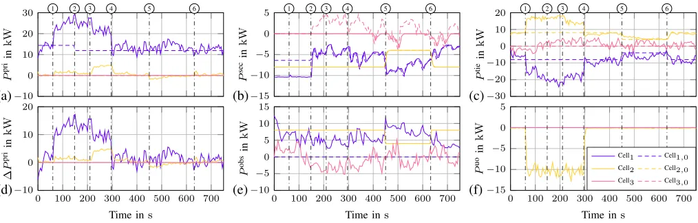
Fig. 9. Resulting primary (a), secondary (b), tieline (c), primary deviation (d), observable (e), and unobservable (f) powers of the DLFC laboratory experiment.

the primary resources covering the unobserved Mobile Load 1 and the missing balancing power of Cell 2 (discussed later). Commencing state publishing of Ppri,c _and ˇ_kc _{between the} Cells at event 3 enabled load sharing due to the alignment of the reference frequency setpoints, which returned towards f0 after turning off Mobile Load 1 at event 4. As in the

simulations, opening the tieline 1-2 at event 5 appears like turning off state publishing because Cell 3 does have primary resources. The frequency references diverge based on the resources’ response speeds and only realign again after closing the line at event 6. Averaging the frequency between 215 sto

750 syields exactly f¯= 50.0 Hz.

The primary power responses in Fig. 9a show that the primary resources operate around their base setpointsP₀pri,cin times of high observability (between events 4 and 5 and after 6). Having virtually no solar production, the power balancing stage of Cell 2 reacts only to the topological changes, while Cells 1 and 3 meet their respective local demands as the secondary powers in Fig. 9b illustrate. Cell 3, also lacking PV support, is only partly able to match its power demand, as mentioned earlier. This mismatch appears like yet another un-observed load to Cells 1 and 2 and is consequently accounted for by their primary resources. While the frequency control of the DLFC works under partial observability, Fig. 9c confirms that tieline balancing requires high observability if no auxiliary observer is employed. The primary power deviations in Fig. 9d hold the necessary information for indirect frequency observa-tion in each Cell (see (10)) and are exchanged between Cells along with the Cells’ droop capabilities (which are constant and therefore not depicted) for load sharing purposes. The observed powers used in the secondary power balancing are shown in Fig. 9e, and finally Fig. 9f features the output of unobserved (i.e., not directly measured by the DLFC) devices.

VI. CONCLUSIONS ANDFUTURERESEARCH

The analytical and experimental assessments in this research demonstrate the aptness of the proposed LFC approach for dynamically changing power systems. Given the inexorable advances in monitoring and communication infrastructure, using primary resources for secondary control is both feasi-ble and reasonafeasi-ble for managing low-inertia systems. Direct

secondary power regulation allows harnessing the benefits of fast-acting flexibility resources while reducing the number of activations. Consideration of the resources’ capabilities in real time promotes the notion of “plug-and-play,” while scalability is ensured by the neighborhood interaction scheme, which is independent of the network’s total extent. As only power bal-ances are considered, hierarchical structures involving DSOs and aggregators (whose resources may be obfuscated for policy or privacy reasons) can be maintained. While the AGC will remain the secondary control method of choice when only tieline measurements are available, the prospect of a significantly higher degree of observability in future power systems enables all the described advantages of the DLFC.

Future research will address the functional gap between DLFC and AGC. First, deviations of scheduled tieline flows in the wake of unobserved power events must be properly han-dled. This requires a tieline observer which does not impair the advantages of the proposed approach (i.e., tuningless control, decoupled Cell balancing). Second, the ENTSO-E demands from secondary control that the ACE must not overshoot [32]. This can currently not be guaranteed in the proposed approach, e.g., after unobserved events, for which reason the DLFC’s concurrent control actions need to be systematically dampened to comply with regulations.

REFERENCES

[1] P. Tielens and D. Van Hertem, “The relevance of inertia in power systems,”Renew. Sustain. Energy Rev., vol. 55, pp. 999–1009, 2016. [2] A. Adrees, P. N. Papadopoulos, and J. V. Milanovic, “A framework to

assess the effect of reduction in inertia on system frequency response,” in2016 IEEE Power Energy Soc. General Meeting (PESGM), pp. 1–5, July 2016.

[3] H. Chavez, R. Baldick, and J. Matevosyan, “The Joint Adequacy of AGC and Primary Frequency Response in Single Balancing Authority Systems,”IEEE Trans. Sustain. Energy, vol. 6, no. 3, pp. 959–966, 2015. [4] L. Dong, Y. Tang, H. He, and C. Sun, “An Event-Triggered Approach for Load Frequency Control With Supplementary ADP,” IEEE Trans. Power Syst., vol. 32, pp. 581–589, Jan 2017.

[5] European Network of Transmission System Operators for Electricity (ENTSO-E), “Nordic Balancing Philosophy,” tech. rep., June 2016. [6] V. Madani, R. Das, F. Aminifar, J. McDonald, S. S. Venkata, D. Novosel,

[7] V. Lakshmanan, M. Marinelli, J. Hu, and H. W. Bindner, “Provision of secondary frequency control via demand response activation on thermo-statically controlled loads: Solutions and experiences from Denmark,”

Appl. Energy, vol. 173, pp. 470–480, 2016.

[8] C. Ziras, E. Vrettos, and S. You, “Controllability and stability of primary frequency control from thermostatic loads with delays,”J. Mod. Power Syst. Clean Energy, vol. 5, no. 1, pp. 43–54, 2017.

[9] Agency for the Cooperation of Energy Regulators (ACER), “Energy Regulation: A Bridge to 2025,” Sept. 2014. [Online]. Available: http: //www.acer.europa.eu. Accessed on May 11, 2017.

[10] Union of the Electricity Industry - EURELECTRIC, “EURELECTRIC’s vision about the role of Distribution System Operators (DSOs) - A EURELECTRIC paper,” tech. rep., Feb. 2016. [Online]. Available: http://www.eurelectric.org. Accessed on May 18, 2017.

[11] V. Gungor, D. Sahin, T. Kocak, S. Ergut, C. Buccella, C. Cecati, and G. Hancke, “A Survey on Smart Grid Potential Applications and Communication Requirements,” IEEE Trans. Ind. Informat., vol. 9, pp. 28–42, Feb 2013.

[12] European Commission, “Cost-benefit analyses & state of play of smart metering deployment in the EU-27 ,” tech. rep., June 2014. http://eur-lex.europa.eu [Accessed: 01-05-2017].

[13] Council of European Energy Regulators (CEER), “The Future Role of DSOs – A CEER Conclusions Paper,” July 2015. [Online]. Available: http://www.ceer.eu. Accessed on May 11, 2017.

[14] European Distribution Systems Operators’ Association for Smart Grids, “TSO – DSO Management Report,” July 2016. http://www. edsoforsmartgrids.eu [Accessed: 19-03-2017].

[15] L. Olmos, J. I. de la Fuente, J. L. Z. Macho, R. R. Pecharroman, A. M. Calmarza, and J. Moreno, “New design for the Spanish AGC scheme using an adaptive gain controller,”IEEE Trans. Power Syst., vol. 19, pp. 1528–1537, Aug. 2004.

[16] A. Khodabakhshian, M. E. Pour, and R. Hooshmand, “Design of a robust load frequency control using sequential quadratic programming technique,”Int. J. Elect. Power Energy Sys., vol. 40, no. 1, 2012. [17] M. Farahani, S. Ganjefar, and M. Alizadeh, “PID controller adjustment

using chaotic optimisation algorithm for multi-area load frequency control,”IET Control Theory Appl., vol. 6, no. 13, pp. 1984–1992, 2012. [18] H. A. Yousef, K. AL-Kharusi, M. H. Albadi, and N. Hosseinzadeh, “Load Frequency Control of a Multi-Area Power System: An Adaptive Fuzzy Logic Approach,”IEEE Trans. Power Syst., vol. 29, pp. 1822– 1830, July 2014.

[19] S. R. Khuntia and S. Panda, “Simulation study for automatic generation control of a multi-area power system by{ANFIS}approach,”Appl. Soft Comput., vol. 12, no. 1, pp. 333–341, 2012.

[20] A. M. Ersdal, L. Imsland, and K. Uhlen, “Model Predictive Load-Frequency Control,”IEEE Trans. Power Sys., vol. 31, Jan 2016. [21] M. Ma, C. Zhang, X. Liu, and H. Chen, “Distributed Model Predictive

Load Frequency Control of Multi-Area Power System after Deregula-tion,”IEEE Trans. Ind. Electron., vol. 4, no. 1, pp. 1–1, 2016. [22] X. Liu, Y. Zhang, and K. Y. Lee, “Robust distributed MPC for load

frequency control of uncertain power systems,”Control Eng. Practice, vol. 56, pp. 136–147, 2016.

[23] H. Shayeghi, H. A. Shayanfar, and A. Jalili, “Load frequency control strategies: A state-of-the-art survey for the researcher,”Energy Convers. Manag., vol. 50, no. 2, pp. 344–353, 2009.

[24] A. Pappachen and A. Peer Fathima, “Critical research areas on load frequency control issues in a deregulated power system: A state-of-the-art-of-review,”Renewable Sustain. Energy Reviews, vol. 72, no. January 2016, pp. 163–177, 2017.

[25] S. C. Tong, Y. M. Li, and H. G. Zhang, “Adaptive Neural Network Decentralized Backstepping Output-Feedback Control for Nonlinear Large-Scale Systems With Time Delays,” IEEE Trans. Neural Netw., vol. 22, pp. 1073–1086, July 2011.

[26] P. Kundur, N. Balu, and M. Lauby,Power System Stability and Control. EPRI power system engineering series, McGraw-Hill, 1994.

[27] R. D’hulst, J. M. Fern´andez, E. Rikos, D. Kolodziej, K. Heussen, D. Geibelk, A. Temiz, and C. Caerts, “Voltage and frequency control for future power systems: The ELECTRA IRP proposal,” in 2015 International Symposium on Smart Electric Distribution Systems and Technologies (EDST), pp. 245–250, Sep. 2015.

[28] C. Caerts et al., “Specification of Smart Grids high level functional architecture for frequency and voltage control,”ELECTRA Deliverable D3.1. WP3 Scenarios and case studies for future power system, Apr. 2015. [Online]. http://www.electrairp.eu.

[29] V. P. Singh, N. Kishor, and P. Samuel, “Load Frequency Control with Communication Topology Changes in Smart Grid,”IEEE Trans. Ind. Inform., vol. 12, pp. 1943–1952, Oct. 2016.

[30] N. O’Connell, P. Pinson, H. Madsen, and M. O’Malley, “Economic Dispatch of Demand Response Balancing Through Asymmetric Block Offers,”IEEE Trans. Power Syst., vol. 31, July 2016.

[31] A. M. Prostejovsky, O. Gehrke, A. M. Kosek, T. Strasser, and H. W. Bindner, “Distribution Line Parameter Estimation Under Consideration of Measurement Tolerances,” IEEE Trans. Ind. Informat., vol. 12, pp. 726–735, April 2016.

[32] European Network of Transmission System Operators for Electricity (ENTSO-E), “P1 – Policy 1: Load-Frequency Control and Performance,” tech. rep. [Online]. Available: http://www.entsoe.eu. Accessed on May 18, 2017.

Alexander M. Prostejovsky(StM’15) was born in

Vienna, Austria, in 1984. He received the B.Sc. degree in electrical and computer engineering in 2009 and the M.Sc. degree in control engineering (focus on nonlinear control theory) in 2011 from the Vienna University of Technology. Since 2014, he has been pursuing a Ph.D. in electrical engineering at the Technical University of Denmark, where he is investigating applications of increased observability in electric distribution grids.

Mattia Marinelli (M’10–SM’17) was born in

Genoa, Italy, in 1983. He received the B.Sc. and M.Sc. degrees in electrical engineering from the University of Genoa, in 2005 and 2007, respectively, and the European Ph.D. degree in power systems, from the same university in 2011. Since 2012, he has been with the Technical University of Denmark. His research interests include power system integra-tion studies, wind and solar data analysis, electric vehicles, and distributed energy resources modeling.

Michel Rezkalla (StM’15) received the M.Sc.

de-gree in 2014 in electrical engineering from the Polytechnic University of Turin in collaboration with the Grenoble Institute of Technology (INP). He is currently a Ph.D. student in the field of electrical engineering at the Technical University of Den-mark. His research interests include synthetic inertia support, frequency control, and distributed energy resources integration.

Mazheruddin H. Syed(StM’11) was born in

Hy-derbad, India in 1990. He received his B.E. degree in electrical and electronics engineering from Osmania University, India, in 2011 and his M.Sc. degree in electrical power engineering from Masdar Institute of Science and Technology, UAE. Presently, he is a research assistant at the Institute for Energy and En-vironment, the University of Strathclyde, Scotland, working towards his Ph.D. His research interests in-clude demand side management, distributed control, and power hardware in the loop simulations.

Efren Guillo-Sansano(StM13) received his M.Sc.