Nonlinear plasmonics in a two-dimensional plasma layer

PAPER

Nonlinear plasmonics in a two-dimensional plasma layer

Bengt Eliasson1,3_{and Chuan Sheng Liu}2

1 _{SUPA, Physics Department, John Anderson Building, University of Strathclyde, Glasgow G4 0NG, Scotland, UK} 2 _{Chou Kuang Piu College, University of Macau, Avenida da Universidade, Taipa, Macau, Peopleʼs Republic of China} 3 _{Author to whom any correspondence should be addressed.}

E-mail:[email protected]@umac.mo

Keywords:two-dimensional plasmons, modulational instability, rogue waves, graphene, sheet of electrons

Abstract

The nonlinear electron dynamics in a two-dimensional

(2D)

plasma layer are investigated theoretically

and numerically. In contrast to the Langmuir oscillations in a three-dimensional

(3D)

plasma, a

well-known feature of the 2D system is the square root dependence of the frequency on the wavenumber,

which leads to unique dispersive properties of 2D plasmons. It is found that for large amplitude

plasmonic waves there is a nonlinear frequency upshift similar to that of periodic gravity waves

(Stokes

waves). The periodic wave train is subject to a modulational instability, leading to sidebands growing

exponentially in time. Numerical simulations show the breakup of a 2D wave train into localized wave

packets and later into wave turbulence with immersed large amplitude solitary spikes. The results are

applied to systems involving massless Dirac fermions in graphene as well as to sheets of electrons on

liquid helium.

1. Introduction

Two-dimensional(2D)conducting layers have unique plasmonic properties, where the wave frequency of low-energy plasmons(in the long wavelength limit)typically depends on the square root of the wavenumber, and observed 2D plasmons have wave-frequencies most commonly in the THz range or below. Examples of experimental observations include 2D plasmons in a sheet of electrons on liquid helium[1], in silicon inversion layers[2], monolayer graphite[3], single layer graphene on SiC substrates[4,5], epitaxial graphene[6], etc.

Graphene has unique electronic and material[7–10]properties, and plasmons in graphene is now afield of intense research with important applications in optics, electronics, metamaterials, light harvesting, energy storage, THz technology, and so on[11,12]. Experiments have shown that Dirac plasmons in graphene on SiC are hybridized with optical phonons of the SiC substrate[13], while scattering of plasmons off capillary waves (riplons)were observed in an electron sheet on liquid helium[1]. Nonlinear photonics have important applications in graphene with respect to harmonic generation[14], optical and plasmonic bistability[15,16],

broadband optical limiting application[17], four-wave mixing frequency conversion[18], and other nonlinear photonic applications[19]. On the other hand, the self-interaction among large amplitude 2D plasmons and

their sidebands could be an important source of instability and localization of wave energy. For example, the instability of large amplitude plasma waves have been suggested to lead to‘rogue waves’in semiconductor plasmas[20], and optical rogue waves have been observed in semiconductor lasers[21]and other optical systems [22,23]. It has also been proposed that graphene supports optical solitons in a graphene monolayer[24],

dissipative plasmon solitons in multilayer graphene[25]and graphene nanodisk arrays[26].

The aim of this paper is to theoretically and numerically investigate the nonlinear behavior of

large-amplitude plasmons in a 2D plasma layer. The basicfluid equations are presented and motivated in section2. As discussed in section3, the unique dispersive properties of 2D plasmons lead to a similar behavior to surface gravity waves[27–29], such as a nonlinear upshift of the frequency due to harmonic generation, and a modulational instability resulting in the growth of sidebands of the periodic wavetrain. In section4, the theoretical results are compared with a direct numerical simulation of the dynamic system, which also

OPEN ACCESS

RECEIVED

11 January 2016

REVISED

4 April 2016

ACCEPTED FOR PUBLICATION

19 April 2016

PUBLISHED

6 May 2016

Original content from this work may be used under the terms of theCreative Commons Attribution 3.0 licence.

Any further distribution of this work must maintain attribution to the author(s)and the title of the work, journal citation and DOI.

demonstrates the breakup of the periodic wavetrain into localized envelope solitary waves and later into spiky large amplitude structures immersed in wave turbulence. Numerical examples are given for systems involving massless Dirac fermions in graphene and for sheets of electrons on liquid helium. Finally, some conclusions are drawn in section4.

2. Nonlinear

fl

uid model of a two-dimensional plasma layer

Low-energy plasmons, i.e. in the long wavelength and low-frequency limit, may be studied using a hydrodynamic model[11,30], in which the conservation of electrons(charges)is governed by a continuity equation and theirfluid velocity(or alternatively the current density)by a momentum equation. Due to the dynamics of the electrons in a 2D sheet of plasma, the electrostatic potential, which extends also to the out-of-plane dimension, has a particular form which leads to a unique dispersive behavior of the system. The potential is obtained from Poisson’s equation with the electron density concentrated to a 2D plane, and is given by

ò

f

p

= - ¢

-- ¢ ¢

( ) ( ( ) )

∣ ∣ ( )

 

t e n t n r

r r

r r ,

4

,

d , 1

e

0

0 2

where the integral is taken over the 2D plane of the plasma layer. Hereneis the areal electron number density,n0 represents the neutralizing ion background density,eis the magnitude of the electron charge,0is the electric

vacuum permittivity, andòis the mean dielectric constant of the surrounding medium[11]. We choose a

coordinate system such that the plasma layer is in thex-yplane. For a plane wave, where the electron density given byne=n0+ne1withne1=(1 2) ˆneexp(-iwt+ik r· )+complex conjugate, and the potential

f=(1 2) ˆfexp(-iwt +ik r· )+complex conjugate, the Fourier component of the potential is obtained from equation(1)as

fˆ = - _{ˆ ( )}

 

k e

n

1

2 0 e, 2

wherek= kx2+ky2is the magnitude of the wave vector. The factor1 2( k)in equation(2)leads to significantly

different behavior of 2D plasmons compared to the three-dimensional(3D)case, where the corresponding factor1 k2_{gives rise to Langmuir oscillations. The electron dynamics is governed by the continuity and}

momentum equation

¶

¶ + ^· ( )= ( )

n

t n v 0, 3

e

e e

and

f ¶

¶ +( ·^) = ^ ( )



t

D en

v

v v 4 , 4

e

e e 0

0

respectively, whereve=xˆvex+yˆveyis the electronfluid velocity,xandyare unit vectors in thexand

y-directions,Dis the Drude weight[11,31],n0is the mean electron density, and the gradient operator

 = ¶ ¶ + ¶ ¶^ x x y y. Equations(3)and(4)are coupled through the potentialfin equation(1). For Schrödinger electrons with effective massmb, the Drude weight(in SI units)isD=e n2 0 (40mb), while for

massless Dirac fermions, the Drude weight isD=e E2 F (4p 0 2), where the Fermi energy isEF =v kF F,

»

-vF 10 ms6 1is the Fermi speed, andkF = pn0is the Fermi wavenumber.

For analytic convenience in the following section, we assume irrotational potentialflow,ve= ^ye, where

yeis theflow potential, which inserted into equations(3)and(4)gives the two scalar equations,

y ¶

¶ + ^· ( ^ )= ( )

n

t n 0, 5

e

e e

and

y _{y f}

¶

¶ + (^ ) = + ( ) ( )



t

D

en B t

1 2

4

, 6

e

e 2 0

0

for the unknownsneandye. Equations(1),(5)and(6)are coupled systems forf,neandye. In equation(6),B(t)

is an arbitrary function of time, which we can choose to set to zero, since thefluid velocityveis the spatial

gradient ofψand will not depend onB(t), and hence,B(t)will not influence the dynamics ofne. The nonlinearity

y ^

( e)2 2in equation(6)can also give rise to a mean component ofyedepending only on time, which likewise

3. Nonlinear wave-wave interactions

Two major nonlinear effects of large amplitude plasmons are here investigated theoretically: a nonlinear frequency upshift due to harmonic generation, and a modulational instability of the wavetrain leading to sidebands growing exponentially in time during the linear phase. These effects have been investigated in the past with respect to general nonlinear dispersive media[32,33], plasma waves[34–39], and nonlinear water waves

[28]. A full investigation of the nonlinear system would involve the following steps: i)tofind the profile of the nonlinear periodic wavetrain governed by equations(5)–(6)and the corresponding nonlinear frequency(or phase velocity)depending on the wavelength and amplitude. This wavetrain would form a‘lattice’on which small-amplitude, unstable sidebands in the form of Bloch wavesF( )q0 exp(iqs), can develop, whereq0andqsare

carrier and perturbation phases(see definitions below), andF( )q0 is periodic with respect to its argument. ii)To

derive a linearized system of differential equations for the Bloch functionsF( )q0 and corresponding

perturbation frequenciesΩ. The set of Bloch functions for each of the perturbation wave vector would then work as eigenfunctions with corresponding eigenvaluesΩ, whose imaginary part gives the growth rate. While such a direct approach could be implemented numerically, we here follow a somewhat simpler route where the carrier wave and the Bloch functions are expanded up to the second harmonics, and where the results are more easy to interpret. We mention that in a previous study of the parametric instabilities of electron oscillations due to intense laser light[40], higher order Fourier expansions of the sidebands were employed using Floquet theory (analogous to Bloch theory).

3.1. Stokes waves

Stokes’investigation of water waves(see e.g.[27])was the starting point of nonlinear theory of dispersive waves, where he among other results found that the dispersion relation involves the wave amplitude. For large

amplitude periodic waves, the nonlinearities lead to harmonic generation, where the second harmonics are generated by products of thefirst harmonics assin2( )q =(1-cos 2( q)) 2

0 0 ,cos2( )q0 =(1+cos 2( q0)) 2,

andsin( )q0 cos( )q0 =sin 2( q0) 2, whereq0=k0·r-wtis the phase,k0is the wave vector, andωis the

frequency which may depend on the wave amplitude. On the other hand, the beating of the second harmonics by thefirst harmonics givescos 2( q0)sin( )q0 = -( sin( )q0 +sin 3( q0)) 2,

q q = q + q

( ) ( ) ( ( ) ( ))

cos 2 0 cos 0 cos 0 cos 3 0 2,sin 2( q0)sin( )q0 =(cos( )q0 -cos 3( q0)) 2, and

q q = q + q

( ) ( ) ( ( ) ( ))

sin 2 0 cos 0 sin 0 sin 3 0 2. The crucial point is that second harmonic components multiplied

byfirst harmonic components give again components proportional tosin( )q0 andcos( )q0. Such‘secular terms,’

which seemed to drive the linear system resonantly, led Stokes to the conclusion that the frequency must change due to nonlinearity. Using a Stokes expansion includingfirst and second harmonics

q q

= + ˆ ( )+ ˆ ( )

ne n0 ne01cos 0 ne02cos 2 0 andye=yˆe01sin( )q0 +yˆe02sin 2( q0)in equations(5)and(6), and

separating the equations for thefirst and second harmonics, gives

q w y y y

µ - - - =

( ) ( ) nˆ n k ˆ k nˆ ˆ k nˆ ˆ ( )

equation 5 , sin : 1

2 0, 7

e e e e e e

0 01 0 02 01 02 01 02 02 02 01

q w y y

µ - - =

( ) ( ) nˆ n k ˆ k nˆ ˆ ( )

equation 5 , sin 2 0 : 2 e02 4 0 02 e02 02 e01 e01 0, 8

q wy y y

µ - + + =

( ) ( ) ˆ g nˆ ˆ ˆ ( )

k n k

equation 6 , cos 0: e01 e e01 e e 0, 9

0 0 0

2

01 02

and

q wy y

µ - + + =

( ) ( ) ˆ g nˆ ˆ ( )

k n k

equation 6 , cos 2 : 2

2

1

4 0, 10

e e e e

0 02

02

0 0

02 01 2

where we have denotedg_e =2D . Third and higher harmonics were neglected in obtaining equations(7)–

(10). Equations(7)–(10)constitute a non-linear eigenvalue problem fornˆe01,nˆe02,yˆe01andyˆe02, with non-trivial

solutions only if the nonlinear dispersion relation w

w =

+

- -

-( )

( )( ) ( )

Y

Y Y Y

1

1 1 3 2 11

2

0 2

3

2

is fulfilled, where the nonlinearity is given by

y

= ˆ ( )

Y k

D

2 , 12

e

04 01 2

2

and we denotedD2=4w2-2w02, where

The linear dispersion relationw0= g k_e 0is of the same form as for deep water gravity waves ifgeis replaced

by the gravitational constantg[27–29]. In deriving equation(11), we have used that equations(8)–(10)give the relations

w w

= +

-+

ˆ ( )

( ) ( )

⎡ ⎣

⎢ ⎤

⎦ ⎥

n n Y Y

Y

2 1 2 1

1 , 14

e02 0

2

0 2

y = w

+

ˆ

( ) ( )

Y

k Y

2

1 , 15

e02 02

and

w y w

=

-+

ˆ ( )

( )

ˆ

( )

n n Y

Y k

1

1 , 16

e01 0 0 e

2 01

0 2

which inserted into equation(7)gives equation(11). Equation(11)relates the frequencyωto the wave amplitude yˆ_{e01. To the lowest order, the frequency depends on the wave amplitude as}

w w y

w w

» + ˆ » + ˆ ( )

⎛

⎝

⎜⎜ ⎞_⎠⎟⎟ ⎛_⎝⎜ ⎞

⎠ ⎟

k n

n

1 7

4 1

7

4 , 17

e e

2 0

2 04 01

2

0

2 0

2 201

02

which shows a nonlinear upshift of the frequency due to thefinite wave amplitude.

3.2. Modulational instability

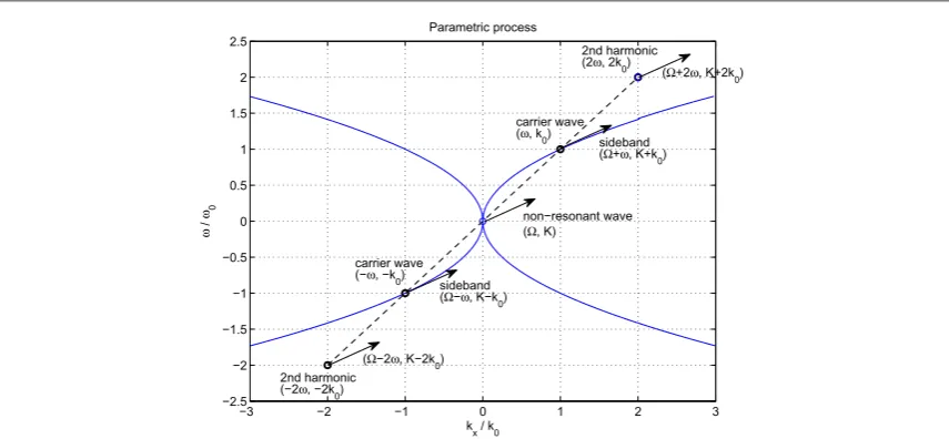
The stability of the system(5)–(6)is investigated by assuming an expansion of the carrier wave and its sidebands as illustrated infigure1. The sidebands at(W  w,Kk0)are almost resonant, i.e. they are located almost on

the dispersion surface of linear waves. The coupling between these almost resonant sidebands by beating of the non-resonant sidebands at(W,K)and(W  2 ,w K2k0)with the large amplitude wave train at(w,k0)and

its second harmonic(2 , 2w k0)forms a feedback loop which gives rise to a modulational instability for certain values ofK. The couplings to second harmonics are crucial to accurately model the modulational instability, and it should be noted that Benjamin and Feir[28]in a similar manner as infigure1included the second harmonics in their treatment of the instability of nonlinear water waves. The nonlinear frequency shift is also important, where the carrier frequencyωis given by the nonlinear dispersion relation(11). The dynamical variables in equations(5)and(6)are Fourier expanded including theirfirst and second harmonics, as well as their sidebands, asne =n0+(1 2)(^ne01eiq0+n^e02e2iq0+^ne+eiq++n^e-eiq-+^neseiqs +n^e2+eiq2+

+ q +

- - )

^

ne2 ei2 complex conjugate andye=(1 2i)(^ye01eiq0+y^e02e2iq0+y^e+eiq++y^e-eiq-+y^eseiqs+y^e2+eiq2+ y

+ q +

- -)

^ _{e complex conjugate}

e2 i2 , whereq0=ik0·r-iwt,qs=iK r· - Wi t,q=qs q0, and

q2=qs 2q0. The respective Fourier component of the potential is obtained by using equation(2). It is

assumed that the sideband componentsnˆe,yˆe,nˆe2,yˆe2,nˆs, andyˆshave much smaller amplitudes thann0, ˆ

ne01,yˆe01,nˆe02, andyˆe02, and thus products among sideband components are neglected. The nonlinear wave

Figure 1.The parametric process, involving the carrier wave at(w,k0)and its second harmonic at(2 , 2w k0), the respective sidebands at(W -w,K-k0),(W +w,K+k0),(W -2 ,w K-2k0),(W +2 ,w K+2k0), and a non-resonant driven mode at(W,K). Since the dynamic variables are real-valued, the carrier frequency and its second harmonic also occur at(-w,-k0)and

w

-

amplitudesnˆe01,yˆe01,nˆe02, andyˆe02are related to each other through equations(12),(14)–(16). Products

between the sidebands and the wavetrain including the carrier waveµeiq0_{and its second harmonic}µ_e2iq0_give rise to relations such as_{e e}iq- iq0=_eiqs,_{e e}iq+ -iq0=_eiqs,_{e e}iq- 2iq0=_eiq+, and_{e e}iq+ -2iq0=_eiq-. Couplings between the second harmonics and the non-resonant sidebands such as_eiq2-_e2iq0=_eiqs_andeiq2+_e-2iq0=_eiqs_{are also}

produced but are numerically found to give only minor contributions to the instability and are therefore neglected here. Separating different Fourier modes gives equations(A1)–(A10)inappendix. The coefficient matrix is on the form of a linear eigenvalue problem for the unknowns(nˆe+,yˆe+,nˆe-,yˆe-,nˆes,yˆes,nˆe2+,yˆe2+,

-ˆ

ne2 ,yˆe2-)where the complex-valued perturbation frequencyW = W + GR i takes the role of an eigenvalue and

where its imaginary partΓis the growth-rate of the instability.

In the numerical solution of the eigenvalue problem, it is assumed(with no loss of generality)thatyˆe01is

real-valued, which leads to that alsonˆe01,nˆe02andyˆe02are also real-valued and are related toyˆe01according to

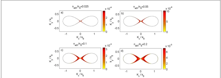
equations(14)–(16); any complex phase factor can be eliminated by a simple change of sideband variables. The wave frequencyωis obtained by solving equation(11)iteratively. A coordinate system is chosen such that the carrier wave propagates in thex-direction,k0=k0x. Amongst the roots given by the system inappendix, we here concentrate on the instability near resonance, where the sidebands(w,k)approximately fulfill the linear dispersion relation, so thatW »R (1 2)(w+-w-)»(1 2)( g ke + - g ke -). The obtained growth-rate for the instability is shown infigure2for different wave amplitudes. For small wave amplitudesnˆe01 n00.1, the

maximum growth-rate depends approximately quadratically on the amplitude, with the maximum growth-rate at an oblique angle to the x-direction. The sidebands have positive growth-rates within a loop-like region in(Kx,

Ky)-space obtained from the resonance conditionsw0= g k_e 0,w+= g ke +, andw-= g ke -as

- + + + + = ( )

⎡ ⎣ ⎢ ⎢ ⎛ ⎝

⎜ ⎞

⎠

⎟ ⎛

⎝ ⎜ ⎞

⎠ ⎟⎤

⎦ ⎥ ⎥

⎡ ⎣ ⎢ ⎢ ⎛ ⎝

⎜ ⎞

⎠

⎟ ⎛

⎝ ⎜ ⎞

⎠ ⎟⎤

⎦ ⎥ ⎥

K k

K k

K k

K k

1 1 2. 18

x y x y

0 2

0 2 1 4

0 2

0 2 1 4

The resonance curve is indicated with dashed lines infigure2. Similar conditions as equation(18)have also been obtained in the theory of nonlinear water waves[41–43]; see for example equation(28)of[43], which in the limit

of infinite depthh ¥reduces to our equation(18).

4. Nonlinear evolution of the system

The nonlinear evolution of the system is investigated by solving the system(5)–(6)numerically in space and time. The 2D spatial simulation domain-10pk x0 10pand-10pk y0 10pis resolved on a

numerical grid with 250 intervals in each direction, and with periodic boundary conditions. A pseudospectral method is employed to accurately calculate spatial derivatives, and to obtain the potential by using the formula

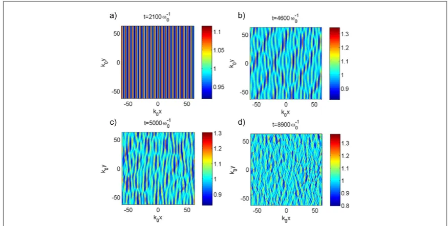
(2)in Fourier space. The standard 4th-order Runge–Kutta method is used to advance the solution in time with the time-stepD =t 0.2w-₀1. Density waves propagating from left to right are excited resonantly to an amplitude about 10% of the background density, seen infigure3(a). Small amplitude random numbers of the order 10−5of the background density are added to the electron density to seed the instability. After a linear growth-phase, the wavetrain is amplitude modulated and breaks up into a train of obliquely propagating solitary waves, seen in

figure3(b), and later into more chaotic behavior(figure3(c)), and into wave turbulence on different length-scales(figure3(d)).

Figure 2.The normalized growth-rateG w0of the modulational instability as a function of the perturbation wave vector(Kx,Ky)for

Figure4shows a comparison between the theoretical growth-rate(taken fromfigure2(c))with the one estimated from the numerical simulation by doing numericalfits to exponentially growing components of the formµexp(Gt). The theoretical and numeric growth-rates show excellent agreement for small wavenumbers. Due to beating with the harmonics of the carrier wave,(_eik r0·,_e2ik r0·, etc), the sidebands appear in a quasi-periodic pattern infigure4(b).

Figure5shows a time-series of the electron densityneat(x y, )=(0, 0). The main features are that the

initially periodic wavetrain(seefigures5(a),(b))becomes unstable and breaks up into a train of localized modulated pulses(figure5(c))and density spikes immersed in wave turbulence(figure5(d)). These spikes have amplitudes several times larger than the mean amplitude of the surrounding waves, which is similar to rogue

Figure 3.The normalized electron densityn ne 0showing(a)a quasi-periodic wavetrain propagating from left to right at time w

=

-t 2100 01,(b)modulated obliquely propagating pulses att=4600w-01,(c)turbulent behavior att=5000w-01, and(d)a cascade to smaller scales with large amplitude spikes immersed in the turbulence at_t=₈₉₀₀w

-01.

waves on the ocean[29]. Figure6shows frequency spectra in time, averaged over all points in thex- andy -directions. The spectrum for earlier timest=0–5000w-₀1(seefigure6(a))shows signatures of harmonic generation and smaller amplitude sidebands of the carrier wave. A small upshift of the carrier frequency

compared to the linear carrier frequencyw =w0is also visible in the inset offigure6(a), which is consistent with

the predicted frequency shift due to second harmonic generation given by equation(17)as indicated with a vertical dashed line in the inset. In the fully nonlinear regime shown infigure6(b)fort=5000–10000w-₀1, the frequency spectrum has evolved into a continuous spectrum with significant components at both higher and lower frequencies compared tow=w0.

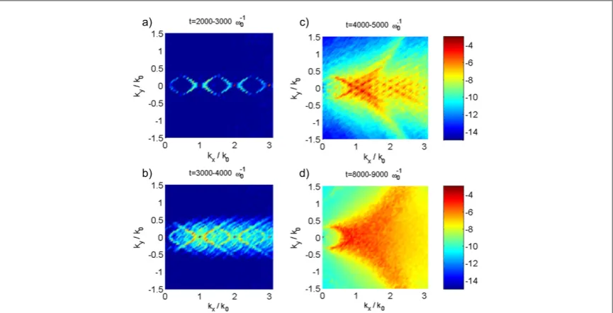
Infigure7, the spatial wave spectrum as a function of(kx,ky)is shown at different times. Due to the harmonic

generation at multiples ofk kx 0= 1andky=0, the wave spectrum initially(figure7(a))attains a

quasi-periodic pattern along the propagation direction. As shown infigures7(b),(c), the sidebands later grow to large amplitudes and the spectrum widens to both higher and lower wavenumbers. Finally, infigure7(d), the spectrum is continuous and broad in particular at large wavenumbers.

Figure 5.(a)The time-series of the electron densityneat(x y, )=(0, 0)showing an instability saturating nonlinearly at

w

»

-t 4500 01. Panels(b)—(d)show close-ups at different times. The instability saturatesfirst by the formation of envelope solitary waves(panel(c))and later isolated, large amplitude pulses(panel(d)).

The regions of instability infigure2are to lowest order similar to the ones of the Benjamin–Feir instability of large amplitude water waves modeled by a nonlinear Schrödinger equation; see e.g.figure 12 of[29]and models taking into account higher order nonlinearity and dispersion[43,44]. Based on the growth-rate of the instability

as shown infigure2, the dynamics may in the limit of long wavelengths/small wavenumbers be phenomenologically modeled by a nonlinear Schrödinger equation of the form

aw ¶

¶ +

¶

¶ +

¶

¶ +

¶

¶ - ∣ ∣ = ( )

⎜ ⎟

⎛ ⎝

⎞ ⎠

A

t c

A

x D

A

x D

A

y A A

i gr x y 0 19

2

2

2

2 0

2

whereA=n n˜e 0is the normalized complex envelope of the wave,n˜erepresents the slowly varying envelop of

the electron density perturbations,cgr= ¶w ¶ =kx w0 2k0is the group velocity of the wave train, and the

group dispersion coefficients areDx=(1 2)¶2w ¶kx2= -w0 (8k02)andDy=(1 2)¶2w ¶ky2=w0 (4k02)

(usingw= g k_e ). The nonlinear Schrödinger equation(19)takes only into account the lowest order dispersive effects, and an assumed cubic nonlinearity amplitude with a coefficient of nonlinearityα. For a monochromatic wave with amplitude∣ ∣A =A0, the nonlinear Schrödinger equation(19)supports a modulational instability

with the growth-rateG =(w0 8k02) 16ak A K02 02( _x2-2K_y2)-(K_x2-2K_y2 2) , which has a maximum of

aw

Gmax = 0A02forKx2-2Ky2=8ak A02 02. By studying instability diagrams such asfigure2and recording the

maximum growth-rate as a function of amplitude, it is found that the coefficient of nonlinearityαis weakly dependent on nonlinearity and decreases withA0asa»0.53 1( +6.5A0)forA0 0.1, givinga»0.5for A0=0.01 anda»0.32forA0=0.1. It should be mentioned that formal methods of the derivation of the nonlinear Schrödinger equation for general nonlinear systems of equations can be found in[32,45,46], for nonlinear water waves in[43,44], and for plasma waves in[33,35–39,47]; we postpone such a formal derivation

of the nonlinear Schrödinger equation(19)to a future work.

We next discuss specific examples of experimental parameters in systems of nonlinear 2D plasmons. As a

first example, we use parameters for massless Dirac Fermions in graphene[11]with an areal number density of electronsn0=10 cm11 -2and a wavenumberk0=0.1kF, where the Fermi wavenumber

p

= = ´

-kF n0 5.6 10 cm5 1. Using the expressions for the Fermi energyEF=v kF F(withvF =10 m s6 -1)

and the Drude weightD=e E2 F (4p 0 2)then gives the wave frequencyw0= 2Dk0  =2.4´10 s13 -1for

a graphene layer with one side exposed to air(1=1)and one side to SiO2(2=3.9)giving

=( + ) =

 1 2 2 2.45. Using the group speedcgr=w0 (2k0)=2.11´10 cm s8 -1and the growth-rate for a

10% wave amplitude(seefigure2(c))G = ´3 10-3w =7.1´10 s

-0 10 1then gives a gain length of

= G » ´

-Lg cgr 3 10 3cm, and the instability would saturate non-linearly within about10Lg » ´3 10-2cm.

The modulational instability typically saturates by initially forming of solitary waves(seefigure2(c))before breaking up into more complicated structures. As an example, equation(19)supports solitary waves propagating along thex-direction of the formA =a eaat sech 2( a a xk )

0 i0 2 0 0 , wherex= -x c tgr . For a 10%

nonlinearity(a0=0.1)the solitary wave would have an electricfield amplitude of(see equation(2))

Figure 7.The spatial wave spectrum(10-logarithmic scale)as a function of(kx,ky)averaged over different times, showing(a)the linear

f

~ ~ ~ ´

-∣ -∣Ex k0 ea n0 0 (2 0 ) 4 10 V cm3 1, and a pulse width in time of the order

a ~

-( a k c )

1 2 0 0 gr 10 12s. Similar electricfield amplitudes(~10 V cm3 -1)have been found theoretically for

dissipative plasmon solitons in multilayer graphene[25]and graphene nanodisk arrays[26]. As a second

example, we consider a plasma layer consisting of an electron sheet on liquid helium[1]with an electron density

=

-n0 10 cm8 2. Here the electrons can be treated as Schrödinger electrons which gives the Drude weight

= (  )

D e n2 0 4 0mb with the effective massmbequal to the free electron massme. A wave frequency

w =₂p´₂₀₀ ´_{10 s}

-0 6 1[1]then gives, usingw0= 2Dk0 with»1, thatk0=10 cm-1. Using the

growth-rateG = ´3 10-3w =3.8´10 s

-0 6 1and the group speedcgr=w0 (2k0)=6.3´10 cm s7 -1gives

the gain lengthLg =cgr G =17 cm. Typical experimental plasmas involving sheets of electrons on liquid

helium have sizes of a few centimeters, which is probably too small to observe the modulational instability in a single pass. However, the modulational instability could potentially develop in the standing wave generated by repeated reflections of the wave against the edges of the plasma.

5. Conclusions and discussion

In conclusion, we have investigated the nonlinear behavior of plasmons in a 2D plasma layer. For a periodic large-amplitude wave, the harmonic generation leads to a nonlinear upshift of the frequency. The large amplitude wave-train is subject to a modulational instability that leads to the growth of sidebands and modulation of the periodic wavetrain. The linear dispersion of the 2D plasmons, as well as their nonlinear frequency upshift and modulational instability, have an interesting analogy in gravity waves such as ocean waves. Direct numerical simulations of the dynamical system confirm both the predicted nonlinear upshift of the frequency and the growth-rate of the modulational instability. The wavetrain eventually breaks up into a series of modulated pulses and more complicated wave turbulence. The spatial and temporal wave spectra show a dual cascade of wave energy to both higher and lower frequencies associated with components at both smaller and larger length-scales.

It has been suggested in the past[34]that large amplitude electron plasma waves in 3D cold electron gaseous plasmas withfixed ions also can undergo a parametric instability with a redistribution of energy from large scales to small-scale sidebands. We carried out a simulation(not shown)similar to that infigure3for this case but could not see any sign of instability. Hence, it seems that the 2D geometry is crucial for the modulational instability of plasmons involving only electrons. In a 3D electron-ion plasma, due to the very low group velocity of the electron oscillations, the coupling to the ion dynamics instead leads to Langmuir wave collapse and strong turbulence[48,49]via the ponderomotive pressure acting on the electrons on a slow time-scale.

Our results show that a modulational instability for plasmons involving massless Dirac fermions in graphene with 10% density variations compared to the background density could give rise to a modulational instability on a typical typical time-scale of the order of a nanosecond and a length-scale of the order 10−3cm. The instability would give rise to large amplitude spikes emersed in wave turbulence, similar as has been observed in optical systems[22,23]. With the advances in graphene fabrication[50], such experiments could potentially be realized in near future.

Acknowledgments

BE acknowledges the hospitality of University of Macau, Macau, PR China, where this work was carried out. This work was partially supported by the EPSRC(UK), grant EP/M009386/1. Discussions with V K Tripathi are gratefully appreciated. The simulation data associated with this paper are available at:http://dx.doi.org/ 10.15129/fb2ab071-2ed2-4718-aafd-c56315764b97.

Appendix. Coupling equations for the sidebands

Separating different Fourier modes in equations(5)and(6)gives the equations for the coefficients of the sidebands as

equation(5),µ_eiq+_:

w y y y

y y y y

- + + +

+ + + + =

+ + + + + +

+ - - + - + + + + +

ˆ ˆ · ˆ ˆ · ˆ ˆ

· ˆ ˆ · ˆ ˆ · ˆ* ˆ · ˆ* ˆ ( )

n n k n n

n n n n

k K k k

k k k k k k k k

1 2

1 2 1

2

1 2

1

2 0 A1

e e e es e es

e e e e e e e e

0 2 01 0 01

equation(6),µ_eiq+_:

w y y y y y y y

- + ++ + + + + =

+ - - + +

ˆ g nˆ _· ˆ ˆ _· ˆ ˆ _· ˆ* ˆ _{( )}

k n k K k k k k

1 2

1

2 0 A2

e e e e es e e e e

0

0 01 0 02 0 2 01 2

equation(5),µ_eiq-_:

w y y y

y y y y

- + + +

+ + + + =

- - -

-+ - + - + - - - -

-ˆ ˆ · ˆ ˆ · ˆ ˆ

· ˆ ˆ · ˆ ˆ · ˆ ˆ · ˆ ˆ ( )

* *

* *

n n k n n

n n n n

k K k k

k k k k k k k k

1 2 1 2 1 2 1 2 1

2 0 A3

e e e es e es

e e e e e e e e

0 2 01 0 01

02 0 02 2 01 2 0 01 2

equation(6),µ_eiq-_:

w y y y y y y y

- - -+ - + + + =

- + + -

-ˆ g nˆ _· ˆ* ˆ _· ˆ* ˆ _· ˆ ˆ _{( )}

k n k K k k k k

1 2

1

2 0 A4

e e e e es e e e e

0

0 01 0 02 0 2 01 2

equation(5),µeiqs_:

y y y y y

-Wnˆ +n K ˆ + 1k-·Knˆ ˆ -+ k+·Knˆ* ˆ ++ k ·Kˆ nˆ-+ k ·Kˆ*nˆ+= ( )

2 1 2 1 2 1

2 0 A5

es 0 2 es e01 e e01 e 0 e01 e 0 e01 e

equation(6),µeiqs_:

y y y y y

-Wˆ + g nˆ + -· ˆ ˆ -+ +· ˆ* ˆ+= ( )

Kn k k k k

1 2

1

2 0 A6

es e es e e e e

0

0 01 0 01

equation(5),µ_eiq2+_:

w y y y

- +nˆ ++n k +ˆ ++ 1k+·k+nˆ ˆ ++ k+·k ˆ nˆ+= ( )

2

1

2 0 A7

e e e e e e

2 2 0 22 2 2 01 2 0 01

equation(6),µ_eiq2+_:

w y y y

- + ++ + + =

+ + +

ˆ g nˆ _· ˆ ˆ _{( )}

k n k k

1

2 0 A8

e e e e e

2 2 2

2 0

0 01

equation(5),µ_eiq2-_:

w y y y

- -nˆ -+n k -ˆ -+ 1k -·k-nˆ* ˆ -+ k-·k ˆ*nˆ-= ( )

2

1

2 0 A9

e e e e e e

2 2 0 22 2 2 01 2 0 01

equation(6),µ_eiq2-_:

w y y y

- - -+ - + =

- -

-ˆ g nˆ _· ˆ* ˆ _{( )}

k n k k

1

2 0 A10

e e e e e

2 2

2

2 0

0 01

wherek=K k0,w= W w,k2=K2k0, andw2= W 2w.

References

[1]Grimes C C and Adams G 1976 Observation of two-dimensional plasmons and electron-ripplon scattering in a sheet of electrons on liquid heliumPhys. Rev. Lett.36145–8

[2]Allen S J Jr, Tsui D C and Logan A R 1977 Observation of the two-dimensional plasmon in silicon inversion layersPhys. Rev. Lett.38 980–3

[3]Nagashima A, Nuka K, Itoh H, Ichinokawa T, Oshima C, Otani S and Ishizawa Y 1992 Two-dimensional plasmons in monolayer graphiteSolid State Commun.83581–5

[4]Liu Y, Willis R F, Emtsev K V and Seyller T 2008 Plasmon dispersion and damping in electrically isolated two-dimensional charge sheetsPhys. Rev.B78201403(R)

[5]Shin S Y, Kim N D, Kim J G, Kim K S, Noh D Y, Kim Kwang S and Chung J W 2011 Control of theπplasmon in a single layer graphene by charge dopingAppl. Phys. Lett.99082110

[6]Lu J, Loh K P, Huang H, Chen W and Wee A T S 2009 Plasmon dispersion on epitaxial graphene studied using high-resolution electron energy-loss spectroscopyPhys. Rev.B80113410

[7_]Novoselov K S, Geim A K, Morozov S V, Jiang D, Zhang Y, Dubonos S V, Grigorieva I V and Firsov A A 2004 Electric_field effect in atomically thin carbonfilmsScience306666–9

[8]Novoselov K S, Jiang D, Schedin F, Booth T J, Khotkevich V V, Morozov S V and Geim A K 2005 Two-dimensional atomic crystalsProc. Natl Acad. Sci. USA10210451–3

[9]Novoselov K S, Geim A K, Morozov S V, Jiang D, Katsnelson M I, Grigorieva I V, Dubonos S V and Firsov A A 2005 Two-dimensional gas of massless Dirac fermions in grapheneNature438197–200

[10]Ulstrup Set al2014 Ultrafast dynamics of massive Dirac fermions in bilayer graphenePhys. Rev. Lett.112257401

[11]Grigorenko A N, Polini M and Novoselov K S 2012 Graphene plasmonicsNat. Photon.6749–58

[12]Luo X, Qiu T, Lu W and Ni Z 2013 Plasmons in graphene: recent progress and applicationsMater. Sci. Eng.R74351–76

[13]Koch R J, Seyller T and Schaefer J A 2010 Strong phonon-plasmon coupled modes in the graphene/silicon carbide heterosystemPhys. Rev.B82201413

[15_]Peres N M R, Bludov Yu V, Santos J E, Jauho A-P and Vasilevskiy M I 2014 Optical bistability of graphene in the terahertz rangePhys. Rev.B90125425

[16]Christensen T, Yan W, Jauho A-P, Wubs M and Mortensen N A 2015 Kerr nonlinearity and plasmonic bistability in graphene nanoribbonsPhys. Rev.B92121407(R)

[17]Wang J, Hernandez Y, Lotya M, Coleman J N and Blau Werner J 2009 Broadband nonlinear optical response of graphene dispersions Adv. Mater.212430–5

[18]Wu Yet al2015 Generation of cascaded four-wave-mixing with graphene-coated microfiberPhoton. Res.3A64–8

[19]Yamashita S 2012 A tutorial on nonlinear photonic applications of carbon nanotube and grapheneJ. Lightwave Technol.30427–47

[20]Yahia M E, Tolba R E, El-Bedwehy N A, El-Labany S K and Moslem W M 2015 Rogue waves lead to the instability in GaN semiconductorsSci. Rep.512245

[21]Zamora-Munt J, Garbin B, Barland S, Giudici M, Leite J R R, Masoller C and Tredicce J R 2013 Rogue waves in optically injected lasers: Origin, predictability, and suppressionPhys. Rev.A87035802

[22]Solli D R, Ropers C, Koonath P and Jalali B 2007 Optical rogue wavesNature4501054–7

[23]Montina A, Bortolozzo U, Residori S and Arecchi F T 2009 Non-Gaussian statistics and extreme waves in a nonlinear optical cavity Phys. Rev. Lett.103173901

[24]Nesterov M L, Bravo-Abad J, Yu A, Nikitin F J, García-Vidal and Martin-Moreno L 2013 Graphene supports the propagation of subwavelength optical solitonsLaser Photon. Rev.7L7–11

[25]Smirnova D A, Shadrivov I V, Smirnov A I and Kivshar Y S 2014 Dissipative plasmon-solitons in multilayer grapheneLaser Photon. Rev. 8291_–6

[26_]Smirnova D A, Noskov R E, Smirnov L A and Kivshar Y S 2015 Dissipative plasmon solitons in graphene nanodisk arraysPhys. Rev.B91 075409

[27]Whitham G B 1974Linear and Nonlinear Waves(New York: Wiley)

[28]Benjamin T B and Feir J E 1967 The disintegration of wave trains on deep water: 1. TheoryJ. Fluid Mech.27417–30

[29]Kharif C and Pelinovsky E 2003 Physical mechanisms of the rogue wave phenomenonEur. J. Mech. B Fluids22603–34

[30]Giuliani G F and Vignale G 2005Quantum Theory of the Electron Liquid(Cambridge: Cambridge University Press)

[31]Abedinpour S H, Vignale G, Principi A, Polini M, Tse W-K and MacDonald A H 2011 Drude weight, plasmon dispersion, and ac conductivity in doped graphene sheetsPhys. Rev.B84045429

[32]Karpman V I and Krushkal E M 1969 Modulated waves in nonlinear dispersive mediaSoviet Phys. J. High Energy Phys.28277–81 [33]Kakutani T and Sugimoto N 1974 Krylov-Bogoliubov-Mitropolsky method for nonlinear wave modulationPhys. Fluids171617–25

[34]Sturrock P A 1957 Non-linear effects in electron plasmasProc. R. Soc. Lond.A242277–99 Sturrock P A 1961Nucl. Energy Part C: Plasma Phys.2158–63

[35]Hasegawa A 1970 Stimulated modulational instabilities of plasma wavesPhys. Rev.A11746–50

[36]Kourakis I and Shukla P K 2005 Exact theory for localized envelope modulated electrostatic wavepackets in space and dusty plasmas Nonlin. Proc. Geophys12407–23

[37]Kourakis I and Shukla P K 2005 Nonlinear propagation of electromagnetic waves in negative-refraction-index composite materials Phys. Rev.E72016626

[38_]Sultana S and Kourakis I 2011 Electrostatic solitary waves in the presence of excess superthermal electrons: modulational instability and enveloüe soliton modesPlasma Phys. Control. Fusion53045003

[39_]McKerr M, Kourakis I and Haas F 2014 Freak waves and electrostatic wavepacket modulation in a quantum elecron-positron-ion plasmaPlasma Phys. Control. Fusion56035007

[40]Quesnel B, Mora P, Adam J C, Héron A and Laval G 1997 Electron parametric instabilities of ultraintense laser pulses propagating in plasmas of arbitrary densityPhys. Plasmas43358–68

[41]Phillips O M 1960 On the dynamics of unsteady gravity waves offinite amplitude: 1. The elementary interactionsJ. Fluid Mech.9 193–217

[42]McLean J W 1982 Instabilities offinite-amplitude gravity waves on water offinite depthJ. Fluid Mech.114331–41

[43]Trulsen K and Dysthe K B 1996 A modified nonlinear Schrödinger equation for broader bandwidth gravity waves on deep waterWave Motion24281–9

[44]Dysthe K B 1979 Note on a modification to the nonlinear Schrödinger equation for application to deep water wavesProc. R. Soc. Lond.A 369105–14

[45]Taniuti T and Yajima N 1969 Perturbation method for a nonlinear wave modulationI, J. Math. Phys.101369–72

[46]Asano N, Taniuti T and Yajima N 1969 Perturbation method for a nonlinear wave modulationII, J. Math. Phys.102020–4

[47]Sen A, Karney C F F, Johnston G L and Bers A 1978 Three-dimensional effects in the non-linear propagation of lower-hybrid waves Nucl. Fusion18171–9

[48_]Zakharov V E 1972 Collapse of Langmuir wavesSoviet Phys. J. High Energy Phys.35908_–14

[49_]Thornhill S G and ter Haar D 1978 Langmuir turbulence and modulational instabilityPhys. Rep.4343_–99