Classification of Partial Discharge EMI Conditions
Using Permutation Entropy-based Features
Imene Mitiche, Gordon Morison and Alan Nesbitt
School of Engineering andBuilt Environment Glasgow Caledonian University
Glasgow, UK
Philip Boreham
Doble EngineeringGuildford, UK
Brian G. Stewart
Institute of Energy and Environment Department of Electronic and Electrical Engineering
University of Strathclyde Glasgow, UK
Abstract—In this paper we investigate the application of feature extraction and machine learning techniques to fault identification in power systems. Specifically we implement the novel application of Permutation Entropy-based measures known as Weighted Permutation and Dispersion Entropy to field Electro-Magnetic Interference (EMI) signals for classification of dis-charge sources, also called conditions, such as partial disdis-charge, arcing and corona which arise from various assets of different power sites. This work introduces two main contributions: the application of entropy measures in condition monitoring and the classification of real field EMI captured signals. The two simple and low dimension features are fed to a Multi-Class Support Vector Machine for the classification of different discharge sources contained in the EMI signals. Classification was performed to distinguish between the conditions observed within each site and between all sites. Results demonstrate that the proposed approach separated and identified the discharge sources successfully.
I. INTRODUCTION
Condition monitoring of high voltage power plants plays an important role for the owning companies. Power systems are a compound of generators, motors, transformers, and cables that jointly contribute to power generation [1]. Failure in any of these assets may be critical causing the whole system to go down resulting in high maintenance and replacement costs, in addition to increased risk for the field workers leading to fines and civil complaints [2]. These failures are often due to defects that occur in different types. Partial Discharge (PD) is an indication of insulation degradation which is considered dangerous for an asset [3]. It is seen as the most significant tool for insulation condition assessment [4]. Corona is another fault which falls under the category of PD discharge sources [2]. Arcing is a further electrical discharge that occurs through an insulating medium [5] when electric current is transmitted through gas. These two latter faults are very common in power transformers [6]. This paper investigates faults that occur due to insulation problem including PD [7] and arcing. EMI is the method employed to capture external discharges on the insulation area or in the air [8]. Early detection of the defects would allow decision making to circumvent the previously cited consequences. Most significantly it will benefit the power plant companies from maximising return of investment, revenue and business profit. Modern solutions for PD fault detection involve machine learning classification
Permu-tation Entropy (WPE) from a number of EMI discharge faults signals. The two features are fed into a Multi-Class Support Vector Machine (MC-SVM) classifier in order to separate the multiple EMI sources. The data was collected from three different high voltage power plants which were reported to contain discharge faults among other conditions. More details regarding discharge sources classification and the database will be discussed later in this paper. The next section introduces the principles of the feature extraction techniques. Section 3 briefly defines the theory of the MC-SVM classifier used for multiple discharge sources separation. Section 4 describes the database and classification approach and presents the results. Finally the last section draws a conclusion on this work and provides suggestions on future work.
II. FEATUREEXTRACTION
A. Weighted Permutation Entropy
WPE is a modified version of PE that combines important information retrieved from a time series in order to save the signal amplitude [19]. First, we denote vectors and scalars by upper and lower case respectively. We consider the time series data X={x1, x2, ..., xN}with lengthN. The time series
is embedded into a space of m dimension and a delay τ
to obtain the vector Xjm,τ ={xj, xj+τ, ..., xj+(m−1)τ};j =
1,2, ..., N−(m−1)τ. For embedded dimensionma number of m! permutation patterns πi are created. Each vector Xj
is mapped to a permutation pattern πi in them dimensional
space and is characterised by weight wj which is calculated
based on the variance of each neighbour’s vectorXjm,τ as:
wj(s) =
1
m m
X
k=1
(x(j+(k−1)τ)−X
m,τ j )
2; s= 1,2, ...S (1)
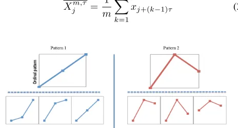
where S is the number of possible amplitude variations that correspond to the same ordinal pattern, as illustrated in Figure 1, and Xjm,τ denotes the mean of Xj which is defined as
follows.
Xjm,τ= 1
m m
X
k=1
[image:2.612.61.293.499.624.2]xj+(k−1)τ (2)
Fig. 1: Various pattern examples corresponding to the same pattern
The weighted probabilities of occurrence for each pattern
πim,τ can then be estimated by:
pw(π m,τ i ) =
P
j≤N1u:type(u)=πi(X
m,τ j ).wj
P
j≤N1u:type(u)∈Π(X
m,τ j ).wj
(3)
where m is the length of sequence to compare and τ is the time delay. The mapping of the symbol to the ordinal pattern is denoted astype(.)and the m!symbols{πim,τ}m!
i denoted
as Π. The indicator function1A(u)of a set Ais defined as:
1A(u) =
(
1 if u∈A
0 if u /∈A
WPE can then be estimated based on Shannon Entropy [20] as:
W P E(m, τ) =− X i:πim,τ∈Π
pw(π m,τ
i ).log(pw(π m,τ
i )) (4)
WPE has previously been exploited to analyse non-linear time series [21] which is our motivation to investigate its performance as a feature for the discharge sources since they exhibit non-stationary nature.
B. Dispersion Entropy
DE was developed in [22] to overcome (PE) and Sample En-tropy (SE) limitations. SE is claimed to be slow in computation particularly for long time series and PE neglects information of the mean of amplitude values and their variations [23], this PE limitation has also been addressed by considering WPE. DE is computed in the following steps for a time series signal X={x1, x2, ..., xN}, with length ofN, which is mapped toc
classes. First, let X be mapped to Y={y1, y2, ..., yN} using
the Normal Cumulative Distribution Function (NCDF). Next, each yj;j = 1, ..., N is assigned a class from 1 to c linearly
as follows.
zcj=round(c.yj+ 0.5) (5)
This provides N members of the classified time series. Here other linear or non-linear methods can also be employed.
Next, embedding vectorsZim,c with dimensionmand time delay dare created:
Zim,c={zic, z c i+d, ..., z
c
i+(m−1)d}; i= 1,2, ..., N−(m−1)d
(6) The latter is mapped to a dispersion pattern πvov1...vm−1,
amongcmpossible dispersion patterns, in that v
0=zic, v1=
zc
i+d, ..., vm−1=zci+(m−1)d.
The dispersion probability of occurrence for each pattern is then calculated as follows.
(7)
p(πvov1...vm−1)
=
P
i≤N−(m−1)d1u:type(u)=πvov1...vm−1(Z
m,c i ) N−(m−1)d
Finally, the DE value is obtained based on Shannon Entropy as follows.
DE(m, c, d) =−Xp(πvov1...vm−1).log(p(πvov1...vm−1))
III. CLASSIFICATIONALGORITHM
SVM is a regression and binary classification method which was developed in the early 90s by Vapnik [24]. It seeks to locate an optimum plane that separates two groups of data. This algorithm is used extensively because of its ability to deal with large features whilst having high detection accuracy when compared to other classification algorithms such as Neural Networks (NN) and Random Forests [25]. A potential issue with the original SVM is that it was designed for binary classification. This is not suitable for the classification of more than two conditions which is the case in this paper. This was addressed by employing MC-SVM using the One-Against-One (OAO) approach where k(k−1)/2 models are constructed [26]. Each one is trained on two classes, p and
q, as a normal binary classification. The testing is performed through a voting strategy called ”Max Win”. If the test sample is predicted to belong to the pth class then the vote for this
class is incremented by one. The class with the highest vote is selected as the prediction. For an optimum performance, suitable input parameters and kernel function must be used. In this work, a grid search method was employed to find the optimum parameters which appeared to be Radial Basis Function (RBF) with standard deviation σ = 0.5. The RBF equation is expressed as:
K(xi, xj) =e−
||xi−xj||2
2σ2 (9)
wherexi is the data input, yi is the respective label, andi=
1,2, ..., L is the number of data sample. It is assumed that the data points belong to two classes “1”and “-1”. Each data point is non-linearly mapped to a feature space separated by a hyperplane with the basic geometric equation:
f(x) =ω.x+b= 0 (10)
where,
• b is a scalar.
• ω is L-dimensional vector.
The latter are the key parameters to determine the hyperplane position. If b = 0, the hyperplane will pass by the origin. Otherwise, the margin is created or increased. The parallel hyperplanes that separate the two different data classes are defined in Equations 11 and 12 for the first and second class respectively.
ω.x+b= 1 (11)
ω.x+b=−1 (12)
Through geometric calculations, the distance between the hyperplanes i.e. the margin width is |w2|. In order to maximise it|w|should be minimised which brings in the criteria:w.xi+ b≥1for the first class orw.xi+b≥ −1for the second one.
This will force the points from each class not to exceed the class hyperplanes i.e. the support vectors. The samples located on the hyperplanes are named support vectors.
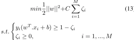
The hyperplane is obtained as a solution to the optimisation problem in Equation 13 by taking into consideration the noise
slack variableζi and the error penaltyC which was set as an
optimum value ofC= 1.05in this work based on the findings of a grid search.
min1
2||w||
2+C
M
X
i=1
ζi (13)
s.t.
(
yi(wT.xi+b)≥1−ζi
ζi≥0, i= 1, ..., M
where ζi represents the distance between the margin and
the data point xi which is in error.
IV. APPLICATION
A. The database
The signals were measured through a High Frequency Current Transformer (HFCT) connected around the neutral earth cable of the asset in order to pick up electromagnetically the PD signals. The latter were recorded at a sampling rate of 24kHz using a PDS200 tool which follows the CISPR16 standard for frequency measurement. The PDS200 is a PD surveyor device which detects and analyses EMI radiations in addition to Radio Frequency Interference (RFI). It employs Quasi peak detection which provides the frequency spectrum of the captured EMI signals. The time resolved data are obtained for further analysis based on the peaks of interest in the frequency spectrum provided by the PDS200. The most common approach is to convert time signals to audio format which are examined by EMI experts in order to identify and label the conditions contained in the signals. These “expert”labels are used for training the classification algorithm. The data was obtained from three different power plants and is described as follows.
1) Site 1: The data was recorded from the Neutral Earth of the generator and includes a total number of 13 files where each one contains 500 cycles over 10 seconds duration.
2) Site 2: The data collected at this site includes 9 files of 500 cycles from which 6 were recorded from a generator, 2 from an Isolated-Phase Bus and 1 from a transformer.
3) Site 3: The data collected at this site includes 8 files of 500 cycles from which 6 were recorded from a generator and 2 from an Isolated-Phase Bus.
[image:3.612.346.561.96.161.2]The identified EMI conditions contained within the data for each site are listed in Table II. The faults’ notation are defined in Table I.
TABLE I: faults’ labels
Fault Label
Arcing A
Corona C
Data Modulation D
Exciter E
Minor m
Noise N
Non-Variable Frequency Drive NVFD Partial Discharge PD
TABLE II: Detected faults in each site
Site Faults
1 C, N, PN, mPD
2 mPD+mA, PD+mA, PD+A, PD, PN, D 3 E+mPD+D, PN, NVFD, PD, E+mPD,E
B. Methodology
The captured data are not sufficient to use with the machine learning algorithm. Thus, the signals were split into smaller segments of 4000 samples in order to have more instances for the classifier. WPE and DE are computed over the segments as features to quantify the signature of each unique condition. This provided a total of 60 instances per signal with two features. The feature vectors are then implemented in the MC-SVM OAO algorithm for classification. The ML models are trained and tested using a ten-fold hold-on cross validation method where 10% of the total data set are held for testing and the remaining 90%are used for training.
C. Results
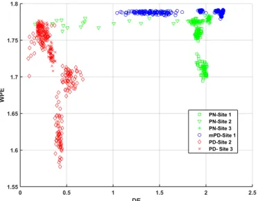
The feature space of DE versus WPE was plotted for each site as well as for the common conditions between all sites. The common conditions are a subset of the measured data in the three sites. With the help of feature extraction, the time domain signals were mapped to a different space that helps to distinguish between the multiple conditions. Figure 2 illustrates the feature space of Site 1 data. It is observed that there is an overlap between N, C, C+E and mPD conditions which may degrade the classification accuracy. Similar overlap occurs on Site 2 feature space in Figure 3. The classification performance in this site might be lower than Site 1 because the overlap seems to be more significant. On the contrary, Figure 4 illustrates clear separation of the feature clusters in Site 3. Thus, high classification accuracy is expected here. Figure 5 shows that the three common conditions can be well separated using these two features only. It is observed that all PD features are concentrated in the range of DE=[0.1-0.8] and they are spread across WPE= [1.57-1.77]. Most of the PN features are clustered around DE=2 and WPE=[1.7-1.78], however a few instances are spread over DE=[0.1-1.7] where some overlap with PD occurs. The significant finding from Figure 5 is that PD instances can be grouped and distinguished from the other conditions regardless of the sites in which the data was captured. The separation in the feature space plots is validated by the classification accuracy results presented in Table III.
[image:4.612.336.530.62.214.2]The top accuracy (99%) was achieved for Site 3 and all sites as expected from the 2-D feature space plots. In second place comes Site 1 with a good performance of 96%. The lowest accuracy (92%) was obtained for Site 2, still this is considered as a good performance. Although the classification accuracy was lower for Site 1 and 2, it was potentially higher as the later contained only a subset of the conditions that occurred during the data collection at all sites.
[image:4.612.339.528.261.414.2]Fig. 2: Feature space of Site 1 data
[image:4.612.336.529.457.621.2]Fig. 3: Feature space of Site 2 data
Fig. 4: Feature space of Site 3 data
TABLE III: Classification Results using WPE and DE features
Site Accuracy%
1 96%
2 92%
3 99%
[image:4.612.363.512.661.714.2]Fig. 5: Feature space of Sites 1, 2 and 3 data
V. CONCLUSIONS
In this paper a novel application of DE and WPE features combined with MC-SVM was investigated on EMI real field captured data for discharge source classification. The feature space plots demonstrate that the different conditions contained in EMI data can be separated with minor overlap using the two entropy measures and it is possible to establish their clas-sification using the MC-SVM algorithm with good accuracy. The significant contributions in this paper are the classification of EMI field captured data and the classification of the same discharge type within different sites. It is important to highlight that the top classification accuracy was achieved between the sites in addition to classification in Site 3. This brings to conclusion that the proposed approach may be exploited for EMI condition monitoring for power plant assets. This work opens possible suggestions to further separate the overlap-ping conditions using other feature extraction techniques and second stage classification for fault prognosis and alerting. Investigation of feature extraction techniques to identify fault location can also be conducted.
REFERENCES
[1] W. Z. E. Kuffel and J. Kuffel, “Chapter 1 -introduction,” in High Voltage Engineering Fundamentals (Second edition), second edition ed., E. Kuffel, W. Zaengl, and J. Kuffel, Eds. Oxford: Newnes, 2000, pp. 8 – 76.
[2] G. Robles, E. Parrado-Hernndez, J. Ardila-Rey, and J. M. Martnez-Tarifa, “Multiple partial discharge source discrimination with multiclass support vector machines,”Expert Systems with Applications, vol. 55, pp. 417 – 428, 2016.
[3] F. Kreuger, inIndustrial High Voltage: 4. Coordinating, 5. Testing, 6. Measuring, second edition ed. Delft University Press, 1992. [4] M. L. R. Bodega, P. H. F. Morshuis and F. J. Wester, “Pd recurrence
in cavities at different energizing methods,” IEEE Transactions on Instrumentation and Measurement, vol. 53, pp. 251–258, 2004. [5] R. Spyker, D. L. Schweickart, J. C. Horwath, L. C. Walko, and
D. Grosjean, “An evaluation of diagnostic techniques relevant to arcing fault current interrupters for direct current power systems in future aircraft,” inProceedings Electrical Insulation Conference and Electrical Manufacturing Expo, 2005., Oct 2005, pp. 146–150.
[6] W. Tang and Q. Wu, inCondition Monitoring and Assessment of Power Transformers Using Computational Intelligence, second edition ed., 1992.
[7] W. Z. E. Kuffel and J. Kuffel, “Chapter 2 - generation of high voltages,” in High Voltage Engineering Fundamentals (Second edition), second edition ed., E. Kuffel, W. Zaengl, and J. Kuffel, Eds. Oxford: Newnes, 2000, pp. 8 – 76.
[8] M. Seltzer-Grant, R. Mackinlay, L. Renforth, and R. Shuttleworth, “New techniques for on-line partial discharge testing of solid-insulated outdoor mv and hv plant,” in2007 42nd International Universities Power Engineering Conference, Sept 2007, pp. 486–489.
[9] S. A. Sureshjani and M. Kayal, “A novel technique for online partial discharge pattern recognition in large electrical motors,” in2014 IEEE 23rd International Symposium on Industrial Electronics (ISIE), June 2014, pp. 721–726.
[10] J. A. Hunter, P. L. Lewin, L. Hao, C. Walton, and M. Michel, “Au-tonomous classification of pd sources within three-phase 11 kv pilc cables,” IEEE Transactions on Dielectrics and Electrical Insulation, vol. 20, pp. 2117–2124, 2013.
[11] M. Majidi, M. S. Fadali, M. Etezadi-Amoli, and M. Oskuoee, “Partial discharge pattern recognition via sparse representation and ann,”IEEE Transactions on Dielectrics and Electrical Insulation, vol. 22, pp. 1061– 1070, 2015.
[12] S. Zhang, C. Li, K. Wang, J. Li, R. Liao, T. Zhou, and Y. Zhang, “Improving recognition accuracy of partial discharge patterns by image-oriented feature extraction and selection technique,”IEEE Transactions on Dielectrics and Electrical Insulation, vol. 23, pp. 1076–1087, 2016. [13] B. Karthikeyan, S. Gopal, and M. Vimala, “Conception of complex probabilistic neural network system for classification of partial discharge patterns using multifarious inputs,” Expert Systems with Applications, vol. 29, pp. 953 – 963, 2005.
[14] N. H. N. Ali, M. Giannakou, R. D. Nimmo, P. L. Lewin, and P. Rapisarda, “Classification and localisation of multiple partial dis-charge sources within a high voltage transformer winding,” in2016 IEEE Electrical Insulation Conference (EIC), June 2016, pp. 519–522. [15] D. Evagorou, A. Kyprianou, P. L. Lewin, A. Stavrou, V. Efthymiou,
A. C. Metaxas, and G. E. Georghiou, “Feature extraction of partial dis-charge signals using the wavelet packet transform and classification with a probabilistic neural network,”IET Science, Measurement Technology, vol. 4, pp. 177–192, 2010.
[16] J. A. Hunter, L. Hao, P. L. Lewin, D. Evagorou, A. Kyprianou, and G. E. Georghiou, “Comparison of two partial discharge classification methods,” inElectrical Insulation (ISEI), Conference Record of the 2010 IEEE International Symposium on, June 2010, pp. 1–5.
[17] Z. Wang, S. McConnell, R. S. Balog, and J. Johnson, “Arc fault signal detection - fourier transformation vs. wavelet decomposition techniques using synthesized data,” in 2014 IEEE 40th Photovoltaic Specialist Conference (PVSC), June 2014, pp. 3239–3244.
[18] M. A. Talib, N. A. Muhamad, and Z. A. Malek, “Fault classification in power transformer using polarization depolarization current analysis,” in 2015 IEEE 11th International Conference on the Properties and Applications of Dielectric Materials (ICPADM), July 2015, pp. 983– 986.
[19] B. Fadlallah, B. Chen, A. Keil, and J. Pr´ıncipe, “Weighted-permutation entropy: A complexity measure for time series incorporating amplitude information,”Physical Review E, vol. 87, p. 022911, 2013.
[20] P. Rathie and S. D. Silva, “Shannon, levy, and tsallis: a note,”Applied Mathematical Sciences, vol. 2, pp. 1359 – 1363, 2008.
[21] J. Xia, P. Shang, J. Wang, and W. Shi, “Permutation and weighted-permutation entropy analysis for the complexity of nonlinear time se-ries,”Communications in Nonlinear Science and Numerical Simulation, vol. 31, pp. 60 – 68, 2016.
[22] M. Rostaghi and H. Azami, “Dispersion entropy: A measure for time-series analysis,”IEEE Signal Processing Letters, vol. 23, pp. 610–614, 2016.
[23] M. Zanin, L. Zunino, O. A. Rosso, and D. Papo, “Permutation entropy and its main biomedical and econophysics applications: A review,” Entropy, vol. 14, pp. 1553–1577, 2012.
[24] V. Vapnik, “The nature of statistical learning theory,” 1995.
[25] J. Lesniak, R. Hupse, R. Blanc, N. Karssemeijer, and G. Szkely, “Comparative evaluation of support vector machine classification for computer aided detection of breast masses in mammography,”Physics in Medicine and Biology, vol. 57, pp. 2560 – 2574, 2012.