City, University of London Institutional Repository
Citation
:
Glock, C.H., Ries, J.M. & Schwindl, K. (2015). Ordering policy for stock-dependent demand rate under progressive payment scheme: a comment. International Journal of Systems Science, 46(5), pp. 872-877. doi: 10.1080/00207721.2013.798446This is the accepted version of the paper.
This version of the publication may differ from the final published
version.
Permanent repository link:
http://openaccess.city.ac.uk/17121/Link to published version
:
http://dx.doi.org/10.1080/00207721.2013.798446Copyright and reuse:
City Research Online aims to make research
outputs of City, University of London available to a wider audience.
Copyright and Moral Rights remain with the author(s) and/or copyright
holders. URLs from City Research Online may be freely distributed and
linked to.
1
Ordering policy for stock-dependent demand rate under progressive payment scheme: A comment
Christoph H. Glock
Department of Law and Economics, Technische Universität Darmstadt ([email protected])
Jörg M. Ries
Department of Law and Economics, Technische Universität Darmstadt ([email protected])
Kurt Schwindl
University of Applied Sciences Würzburg-Schweinfurt ([email protected])
Abstract: In a recent paper, Soni and Shah [2009. Ordering policy for stock-dependent demand rate under progressive payment scheme. International Journal of Systems Science 40, 81-89] developed a model for finding the optimal ordering policy for a retailer facing stock-dependent demand and a supplier offering a progressive payment scheme. In this note, we correct several errors in the formulation of the models of Soni and Shah and modify some assumptions to increase the model’s applicability. Numerical examples illustrate the benefits of our modifications.
Keywords: Economic order quantity (EOQ); stock-dependent demand; progressive credit periods; trade credit
Introduction
In a recent paper, Soni and Shah (2009) developed a model for finding the optimal ordering policy for a retailer facing stock-dependent demand and a supplier offering a progressive payment scheme.1 They assumed that in case the retailer pays before time M, the supplier does not charge any interest to the retailer, whereas in case the retailer pays between times M and N
with M < N, the supplier charges an interest rate Ic1. In case the retailer pays after time N, the supplier charges an interest rate Ic2, with Ic2 > Ic1. In practice, the retailer often uses inventory as collateral to get a low-interest loan from a supplier (or a bank). However, in this case, the supplier is willing to provide a loan without any collateral or monthly payment. Revenues the retailer receives from selling products to the end customer may be deposited in an interest-bearing account until the account is completely settled2, which leads to interest earnings at the rate of Ie. The authors assumed that in case the retailer is not able to settle the unpaid balance at time M (or N), s/he will settle as much of the unpaid balance as possible at these points in time. Afterwards, s/he continuously reduces the remaining debt by transferring incoming revenues to the supplier to minimize interest payments. Teng et al. (2011) recently extended Soni and Shah’s model by including some additional aspects such as deterioration, limited capacity and non-zero ending inventory under profit maximization.
While assuming a progressive interest scheme offered to the retailer, Soni and Shah do not consider the case where Ie > Ic1 in their model, although this case is not explicitly excluded in
1 Note that in contrast to what Soni and Shah state on pages 81 and 82 of their paper, demand in their model is
exclusively stock-dependent and does not have a constant fraction.
2 the model assumptions. In the case where the interest rate of the retailer exceeds the interest rate charged by the supplier during the initial credit period (which may be the case in certain industries with a small number of powerful customers, see for example Ng et al., 1999 or Klapper et al., 2012), it is not rational from the retailer’s perspective to settle the unpaid balance at time M. Instead, it would be better to keep the sales revenue in an interest-bearing account (see Summers and Wilson, 2002) and to settle the unpaid balance when the interest charged by the supplier exceeds the incomes from interest. We therefore add an assumption to the model and explicitly assume that the case Ie > Ic1 may occur in addition to the other cases studied by Soni and Shah. However, we exclude the case Ie > Ic2 to avoid scenarios where it would be rational for the retailer never to pay the supplier.
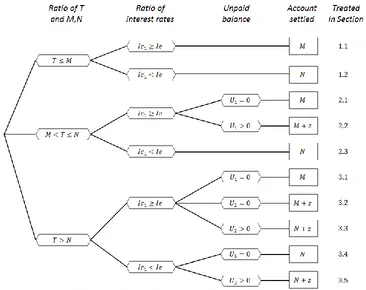
Depending on the ratio of the interest rates Ic1 and Ie and the time when the retailer sells off the entire production lot, ten different cases may arise which are summarized in Figure 1. Note that
[image:3.612.120.486.335.625.2]U1, U2 and U3 denote the unpaid balances at times M and N, respectively, and z the additional time which is required after times M or N to settle the unpaid balance completely. All cases will be discussed briefly in the following with reference to their treatment in the Soni and Shah (2009) paper. In addition, we will correct some errors contained in the original article. If not stated otherwise, we adopt the assumptions and notations used in Soni and Shah (2009) in the following.
Figure 1: Cases for settling the unpaid balance
Modified model
Subcase 1.1: In Case 1 (which is Subcase 1.1 in our comment), Soni and Shah considered a scenario where the entire lot is sold off before the supplier starts charging an interest. If T
3 subcase, the retailer deposits the sales revenue in an interest-bearing account and settles the balance at time M. Correcting an error in the right-hand side of Soni and Shah’s Eq. (7), the interest earned per year can be written as:
𝐼𝐸1,1 =𝑃𝐼𝑒𝑇 (∫ 𝑅(𝑡)𝑡d𝑡 + 𝑄(𝑀 − 𝑇)0𝑇 ) = 𝑃𝐼𝑒𝛼1/(1−𝛽)(1 − 𝛽)1/(1−𝛽)𝑇𝛽/(1−𝛽)(𝑀 − 𝑇
2−𝛽) (1)
As the retailer settles the balance at time M, and therefore does not have to pay interest to the supplier (i.e., IC1,1 = 0), the total costs amount to:
𝑇𝐶1,1 = 𝐴𝑇− 𝐼𝑒𝑃 (𝑀 −2−𝛽𝑇 ) 𝑘1+2−𝛽ℎ𝑘1 (2)
where 𝑘1 = 𝛼1/(1−𝛽)(1 − 𝛽)1/(1−𝛽)𝑇𝛽/(1−𝛽).
The optimal solution to Eq. (2) is the solution of the following non-linear equation (provided that the second derivation of Eq. (2) with respect to T is greater than zero for all T):
d𝑇𝐶1,1
d𝑇 = −
𝐴
𝑇2+
𝐼𝑒𝑃𝑘1
2−𝛽 −
𝐼𝑒𝑃(𝑀−2−𝛽𝑇 )𝛽𝑘1
𝑇(1−𝛽) +
ℎ𝛽𝑘1
𝑇(1−𝛽)(2−𝛽) (3)
Subcase 1.2: For TM and Ie > Ic1, the retailer achieves a financial benefit from postponing the refund and keeping the sales revenue in an interest-bearing account until time N. Between times
M and N, s/he has to pay interest to the supplier. However, due to Ie > Ic1, the interest earned exceeds the interest paid within this period. Similar to Subcase 1.1, the interest earned per year can be calculated as:
𝐼𝐸1,2 =𝑃𝐼𝑒𝑇 (∫ 𝑅(𝑡)𝑡d𝑡0𝑇 + 𝑄(𝑁 − 𝑇)) = 𝑃𝐼𝑒𝛼1/(1−𝛽)(1 − 𝛽)1/(1−𝛽)𝑇𝛽/(1−𝛽)(𝑁 −2−𝛽𝑇 ) (4)
The overall interest cost between M and N, on the other hand, amount to:
𝐼𝐶1,2 = 𝐼𝑐1
𝑇 𝐶𝑄(𝑁 − 𝑀) (5)
The total costs are thus calculated as:
𝑇𝐶1,2 = 𝐴𝑇+ 𝐶𝐼𝑐1(𝑁 − 𝑀)𝑘1− 𝐼𝑒𝑃 (𝑁 −2−𝛽𝑇 ) 𝑘1+ ℎ𝑘1
2−𝛽 (6)
where 𝑘1 = 𝛼1/(1−𝛽)(1 − 𝛽)1/(1−𝛽)𝑇𝛽/(1−𝛽).
The optimal solution to Eq. (6) is the solution of the following non-linear equation (provided that the second derivation of Eq. (6) with respect to T is greater than zero for all T):
d𝑇𝐶1,2
d𝑇 = −
𝐴
𝑇2−
𝐶𝐼𝑐1(𝑁−𝑀)𝛽𝑘1
𝑇(𝛽−1) +
𝐼𝑒𝑃𝑘1
2−𝛽 −
𝐼𝑒𝑃(𝑁−2−𝛽𝑇 )𝛽𝑘1
𝑇(1−𝛽) +
ℎ𝛽𝑘1
4
Subcase 2.1: In the case where M < TN and Ie ≤ Ic1, the retailer settles as much of the unpaid balance as possible at time M to minimize interest payments. In the first subcase, it is assumed that the sum of sales revenue and interest earned at time M is sufficient to settle the unpaid balance, i.e. U1 = 0, where U1 is the buyer’s debt at time M. The interest earned until time M is formulated as follows (note that this formulation corrects an error in the right-hand side of Soni and Shah’s Eq. (11)):
𝐼𝐸2,1 = 𝑃𝐼𝑒𝑇 ∫ 𝑅(𝑡)𝑡d𝑡0𝑀 = 𝑇(2−𝛽)𝑃𝐼𝑒 𝛼1/(1−𝛽)(1 − 𝛽)1/(1−𝛽)(𝑇(2−𝛽)/(1−𝛽)(1 − 𝛽) − (𝑇 −
𝑀)1/(1−𝛽)(𝑀 + 𝑇(1 − 𝛽))) (8)
As the retailer does not have to pay interest to the supplier in this subcase (i.e. IC2,1= 0), the total
costs amount to:
𝑇𝐶2,1 =𝐴𝑇+𝑇(2−𝛽)ℎ𝑘2 +𝐼𝑒𝑃(1−𝛽)𝑘2−𝛽 2−𝐼𝑒𝑃(𝑇−𝑀)
1/(1−𝛽)(𝑀+𝑇(1−𝛽))𝑘 2
(2−𝛽)𝑇(2−𝛽)/(1−𝛽) (9)
where 𝑘2 = 𝛼1/(1−𝛽)(1 − 𝛽)1/(1−𝛽)𝑇1/(1−𝛽).
The optimal solution to Eq. (9) is the solution of the following non-linear equation (provided that the second derivation of Eq. (9) with respect to T is greater than zero for all T):
d𝑇𝐶2,1
d𝑇 = −
𝐴
𝑇2+
ℎ𝛽𝑘2
𝑇2(1−𝛽)(2−𝛽)+
𝐼𝑒𝑃(1−𝛽)𝑘2
2−𝛽 −
𝐼𝑒𝑃(𝑇−𝑀)1 (1−𝛽)⁄ (𝑀+𝑇(1−𝛽))𝑘2
(2−𝛽)𝑇(2−𝛽) (1−𝛽)⁄ +
𝐼𝑒𝑃(1−𝛽)(𝑇−𝑀)1 (1−𝛽)⁄ 𝑘2
(2−𝛽)𝑇(2−𝛽) (1−𝛽)⁄ −
2𝐼𝑒𝑃(1−𝛽)𝛽+1𝑘2
(2−𝛽)𝑇 −
𝐼𝑒𝑃𝛽𝑘2
2−𝛽 +
𝐼𝑒𝑃(𝑇−𝑀)𝛽 (1−𝛽)⁄ (𝑀+𝑇(1−𝛽))𝑘2
(2−𝛽)𝑇(2−𝛽) (1−𝛽)⁄ +
𝐼𝑒𝑃(𝑇−𝑀)1 (1−𝛽)⁄ 𝛽(𝑀+𝑇(1−𝛽))𝑘
2
(2−𝛽)(1−𝛽)𝑇(2−𝛽) (1−𝛽)⁄ (10)
Subcase 2.2: In contrast to Subcase 2.1, we now consider the case where the sum of sales revenue and interest earned at time M is not sufficient to settle the balance completely, i.e. U1 > 0. Thus, the retailer has to pay interest to the supplier. Interest earned is the same as the one given in Eq. (8). In calculating the unpaid balance U1, Soni and Shah assumed that U1=CQ –
(PR(M)M+IE2). R(t), in this context, denotes the stock-dependent demand rate at time t. Since the demand rate decreases in t due to a decreasing inventory level, we note that PR(M)M
underestimates the sales revenue of the retailer, since R(M) < R(M–Δ) for Δ > 0. As a
consequence, U1 has to be reformulated as follows:
𝑈1 = 𝐶𝑄 − (𝑃 ∫ 𝑅(𝑡)d𝑡0𝑀 + 𝑃𝐼𝑒 ∫ 𝑅(𝑡)𝑡d𝑡0𝑀 ) (11)
5 unpaid balance cannot be settled at time M, but before time N, it follows that interest paid as given in Eq. (17) of the Soni and Shah-paper can be reformulated as follows:
𝐼𝐶2,2 =𝐼𝑐1
𝑇 ∫ 𝑈1− 𝑃𝑅(𝑡)(𝑡 − 𝑀)d𝑡 𝑀+𝑧
𝑀 (12)
where M+z denotes the point in time when the unpaid balance has been completely settled, with z
> 0 and M+z < T. The total costs for this case amount to:
𝑇𝐶2,2 =𝐴𝑇+𝑇(2−𝛽)ℎ𝑘2 +𝐼𝑐1𝑇 ∫𝑀𝑀+𝑧𝑈1− 𝑃𝑅(𝑡)(𝑡 − 𝑀)d𝑡+𝐼𝑒𝑃(1−𝛽)𝑘22−𝛽 −𝐼𝑒𝑃(𝑇−𝑀)1/(1−𝛽)(𝑀+𝑇(1−𝛽))𝑘2
(2−𝛽)𝑇(2−𝛽)/(1−𝛽)
(13)
where 𝑘2 = 𝛼1/(1−𝛽)(1 − 𝛽)1/(1−𝛽)𝑇1/(1−𝛽). Due to the indefinite integral, we are unable to calculate an optimality condition for Subcase 2.2 explicitly. However, we note that the value of z
can be approximated numerically with arbitrary precision (e.g. with the help of the bisection method). This permits us to calculate a near-optimal solution numerically for this subcase.
Subcase 2.3: This subcase (i.e. the case where M < T N and Ie > Ic1) is identical to Subcase 1.2.
Subcase 3.1: This subcase (i.e. the case where T > N, Ie ≤ Ic1 and U1 = 0) is identical to Subcase 2.1.
Subcase 3.2: This subcase (i.e. the case where T > N, Ie ≤ Ic1, U1 > 0 and U2 = 0) is identical to Subcase 2.2.
Subcase 3.3: In this subcase, with T > N and Ie ≤ Ic1, the retailer is not able to pay off the total purchase cost at M or N. Thus, s/he will settle as much of the balance as is possible at times M
and N. Between times M and N, the sales revenue is kept in an interest-bearing account, and the supplier charges interest on the outstanding balance U1 with interest rate Ic1. Afterwards, as in
Subcase 2.2, the retailer transfers each dollar s/he earns directly to the supplier who charges interest on the gradually reducing unpaid balance U2 at the interest rate Ic2. As the retailer
partially settles the account in M and N, s/he is able to realize interest earnings in the period [0,
N], which can be calculated as:
𝐼𝐸3,3 = 𝑃𝐼𝑒𝑇 (∫ 𝑅(𝑡)𝑡d𝑡0𝑀 + ∫ 𝑅(𝑡)(𝑡 − 𝑀)d𝑡M𝑁 ) (14)
The unsettled balance U2 (at time N) calculated by Soni and Shah again underestimates the sales revenue of the retailer. Further, while estimating the interest earnings between times M and N,
the authors neglected the time the revenue is kept in the account. Therefore, U2 has to be
reformulated as follows:
6 where U1 is the unpaid balance at time M as given in Eq. (11). Consequently, the interest payable per year, IC3,3, is given as:
𝐼𝐶3,3 =𝐼𝑐1
𝑇 𝑈1(𝑁 − 𝑀) +
𝐼𝑐2
𝑇 ∫ 𝑈2− 𝑃𝑅(𝑡)(𝑡 − 𝑁) d𝑡 𝑁+𝑧
𝑁 (16)
where N+z denotes the point in time when the unpaid balance has been settled, with z > 0 and
N+zT.
The objective function for Subcase 3.3 has the same structure and solution procedure as the one given in Eq. (13), with the exceptions that IC2,2 needs to be substituted by IC3,3 and that the interests earnings IE3,3 have to be considered. Again, a near-optimal solution can be calculated
numerically for this subcase.
Subcase 3.4: If the interest rate of the retailer Ie exceeds the interest charges of the supplier for the first credit period, Ic1, s/he will again not settle the account before N. Instead, the retailer
keeps the sales revenues between times M and N in an interest-bearing account. As the unpaid balance U3 is assumed to be 0 in this subcase, the account is completely settled at time N. Thus, the interest earned is given as:
𝐼𝐸3,4 = 𝑃𝐼𝑒𝑇 ∫ 𝑅(𝑡)𝑡d𝑡0𝑁 =𝐼𝑒𝑃𝛼1/(1−𝛽)𝑇(2−𝛽)(1−𝛽)(2−𝛽)/(1−𝛽)(𝑇(2−𝛽)/(1−𝛽)− (𝑇 − 𝑁)1/(1−𝛽)(𝑁 +
𝑇(1 − 𝛽))) (17)
The interest charges in the period [M, N] amount to:
𝐼𝐶3,4 =𝐼𝑐𝑇1𝐶𝑄(𝑁 − 𝑀) (18)
Thus, the total costs for this subcase are formulated as:
𝑇𝐶3,4 =
𝐴
𝑇+ 𝐶Ic1(𝑁 − 𝑀)𝑘1 + ℎ𝑘1 2 − 𝛽−
𝛽 − 1 𝛽 − 2
Ie𝑃𝛼
𝑇 ((𝑁 − 𝑇)(𝑁 + 𝑇 − 𝑇𝛽)𝑘4𝛽− 𝑇2(𝛽
− 1)𝑘3𝛽)
(19)
where 𝑘1 = 𝛼1 (1−𝛽)⁄ (1 − 𝛽)1 (1−𝛽)⁄ 𝑇𝛽 (1−𝛽)⁄ , 𝑘3 = (𝛼(1 − 𝛽)𝑇) 1
1−𝛽 and 𝑘4 = (𝛼(1 − 𝛽)(𝑇 −
𝑁))1−𝛽1 .
The optimal solution to Eq. (18) is the solution of the following non-linear equation (provided that the second derivation of Eq. (18) with respect to T is greater than zero for all T):
𝑑𝑇𝐶3,4
𝑑𝑇 = −
𝐴
𝑇2+ 𝐶Ic1(𝑁 − 𝑀)𝑇 2𝛽−1
1−𝛽(1 − 𝛽) 𝛽
1−𝛽𝛽 +ℎ𝑇 2𝛽−1
1−𝛽𝛼1−𝛽1 (1−𝛽)1−𝛽𝛽 𝛽
2−𝛽 −
Ie𝑃𝛼(𝛽−1)((𝑁−𝑇)(𝑁+𝑇−𝑇𝛽)𝑘4𝛽−𝑇2(𝛽−1)𝑘
3𝛽)
𝑇2(2−𝛽) +
Ie𝑃𝑇 1+𝛽
1−𝛽𝛼(1−𝛽)
(2−𝛽)𝑘3𝑘4 ((𝑁 − 𝑇)
𝛽 1−𝛽(𝑇
7
𝑁𝑇𝛽−11 )𝛼 1 1−𝛽(𝑇
𝛽
𝛽−1(𝛽 − 1) − 𝑁𝑇 1
𝛽−1)(1 − 𝛽) 𝛽 1−𝛽𝛽𝑘
3𝑘4𝛽+ 𝑇
1
𝛽−1(𝑁𝑇
1
𝛽−1𝛽 − 2𝑇 𝛽 𝛽−1(𝛽 −
1))𝑘3𝑘41+𝛽+ 𝑇 𝛽
𝛽−1(𝛽 − 1)𝑘
3𝛽𝑘4(𝛼
1
1−𝛽(1 − 𝛽) 𝛽
1−𝛽𝛽 + 2𝑇 1
𝛽−1𝑘3)) (20)
Subcase 3.5: For the case where Ie > Ic1 and where the retailer is unable to settle the balance completely at time N, the account is partially settled at time N and hereafter the unpaid balance is continuously reduced by sales revenues until it is completely settled. The interest earnings until time N are the same as those given in Eq. (17).
In addition, the unpaid balance at time N equals:
𝑈3 = 𝐶𝑄(1 + 𝐼𝑐1(𝑁 − 𝑀)) − (𝑃 ∫ 𝑅(𝑡) d𝑡0𝑁 + 𝐼𝑒𝑃 ∫ 𝑅(𝑡)𝑡 d𝑡0𝑁 ) (21)
The interest charges amount to:
𝐼𝐶3,5 =𝐼𝑐𝑇1𝐶𝑄(𝑁 − 𝑀) +𝐼𝑐𝑇2∫𝑁𝑁+𝑧𝑈3− 𝑃𝑅(𝑡)(𝑡 − 𝑁) ⅆ𝑡 (22)
where N+z denotes the point when the unpaid balance has been settled, with z > 0 and N+zT. The objective function for Subcase 3.5 has the same structure and solution procedure as the one given in Eq. (13), with the exception that IC2,2 needs to be substituted by IC3,5 and the interest earning IE3,4 have to be considered. Again, a near-optimal solution can be calculated numerically
for this subcase.
Numerical examples
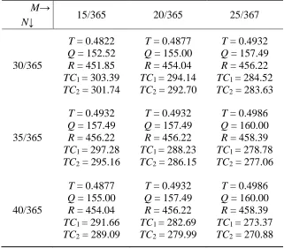
To illustrate the behavior of our model, we consider the parametric values shown in Table 1 and the payment policies of the retailer introduced above. The numerical examples (cf. Table 2) indicate that:
1. For a fixed consumption rate, an increase in the first credit period has only minor influences on the order quantity and the length of the order cycles. The total costs, in turn, are reduced as M adopts higher values. An increase in the second credit period results in higher order quantities, a longer order cycle length and lower total costs.
2. An inverse interest structure with Ie > Ic1 does not affect the lot size policy itself. However, it affects the optimal payment policy of the retailer, who may choose a different point in time to settle the balance. In contrast to the model of Soni and Shah (cf. TC1 in Table 2), the presented payment policy (cf. TC2 in Table 2) may reduce the total costs of the buyer.
Table 1: Model parameters
α = 100 first parameter of the demand function
β = 0.30 second parameter of the demand function
A = 100 ordering cost per order
8
h = 0.20 inventory holding cost per unit and year
Ic1 = 0.10 interest rate per year for the first credit period
Ic2 = 0.18 interest rate per year for the second credit period
Ie = 0.14 interest rate on deposits for the retailer
M = 15 first permissible credit period
N = 30 second permissible credit period
[image:9.612.145.466.249.530.2]P = 30 unit selling price
Table 2: Effect of M and N on decision parameters
M→
15/365 20/365 25/367
N↓
30/365
T = 0.4822
Q = 152.52
R = 451.85
TC1 = 303.39
TC2 = 301.74
T = 0.4877
Q = 155.00
R = 454.04
TC1 = 294.14
TC2 = 292.70
T = 0.4932
Q = 157.49
R = 456.22
TC1 = 284.52
TC2 = 283.63
35/365
T = 0.4932
Q = 157.49
R = 456.22
TC1 = 297.28
TC2 = 295.16
T = 0.4932
Q = 157.49
R = 456.22
TC1 = 288.23
TC2 = 286.15
T = 0.4986
Q = 160.00
R = 458.39
TC1 = 278.78
TC2 = 277.06
40/365
T = 0.4877
Q = 155.00
R = 454.04
TC1 = 291.66
TC2 = 289.09
T = 0.4932
Q = 157.49
R = 456.22
TC1 = 282.69
TC2 = 279.99
T = 0.4986
Q = 160.00
R = 458.39
TC1 = 273.37
TC2 = 270.88
Conclusion
In this comment, we corrected some errors in a recent paper of Soni and Shah (2009) and modified some of its assumptions to increase the model’s applicability. One important modification is that we assumed that the interest charged by the supplier in the first credit period,
9
References
Goyal, S.K., Teng, J.T. and Chang, C.T. (2007), “Optimal ordering policies when the supplier provides a progressive interest scheme”, European Journal of Operational Research, 179 (2), 404-413.
Klapper, L., Laeven, L. and Rajan, R. (2012), “Trade Credit Contracts”, Review of Financial Studies, 25 (3), 838-867.
Ng, C.K., Smith, J.K. and Smith, R.L. (1999), “Evidence on the Determinants of Credit Terms Used in Interfirm Trade”, Journal of Finance, 54 (3), 1109-1129.
Soni, H., and Shah, N. H. (2009), “Ordering policy for stock-dependent demand rate under progressive payment scheme”, International Journal of Systems Science, 40 (1), 81-89.
Summers, B. and Wilson, N. (2002), “An Empirical Investigation of Trade Credit Demand”,
International Journal of the Economics of Business, 9 (2), 257-270.
Teng, J.-T., Krommyda, I.-P., Skouri, K., and Lou, K.-R. (2011), “A comprehensive extension of optimal ordering policy for stock-dependent demand under progressive payment scheme”,